1. Introduction
Traditional methods identify faults by computing specific attributes designed to measure the continuity of seismic reflectors. First-generation coherence techniques, for instance, infer potential fault locations by identifying data discontinuities [
1]. Second-generation coherence algorithms, such as D2, calculate seismic trace similarity using covariance matrices [
2], while third-generation algorithms derive coherence attributes from eigenvalue analysis for seismic fault identification [
3]. However, coherence-based algorithms are susceptible to noise and residual stratigraphic responses. Methods predicated on fault-induced discontinuities, such as variance [
4,
5] and gradient magnitude [
6], also exhibit limitations stemming from their sensitivity to noise and stratigraphic features. Early fault enhancement methods employed computation windows or smoothing directions premised on simplified geometric assumptions [
7,
8,
9]. Given the complex morphology of actual faults, subsequent methods evolved to perform smoothing along the true dip and azimuth of faults, either by directly computing attributes [
10,
11] or by enhancing existing ones [
12,
13,
14]. Nonetheless, these approaches are often computationally demanding. To overcome this challenge, more sophisticated fault enhancement techniques emerged, [
15,
16] as well as optimal surface voting [
17]. Nevertheless, their performance is critically dependent on the quality of initial fault attributes and meticulous parameter tuning, rendering them computationally intensive and prone to generating inaccurate or spurious fault connections in complex geological settings. Dorn and James et al. [
18] integrated geological prior knowledge with digital signal processing techniques to develop an automated fault extraction (AFE) method, which proved effective for identifying large, discontinuous faults. Admasu et al. [
19] proposed the principal contour line technique, which achieved semi-automated fault tracking by combining manual and automated interpretation. Although existing fault identification methods exhibit a degree of intelligence and automation, their efficacy often remains contingent upon the initial selection of attributes and the chosen computational strategies. More fundamentally, these traditional approaches are rooted in a “model-driven” or “rule-based” paradigm. They rely on human experts to pre-define a simplified geophysical or geometric proxy for a fault—such as a surface of discontinuity, a zone of low coherence, or a specific dip and azimuth. The algorithms are then designed to search for patterns that conform to these explicit, pre-defined rules. As exploration targets deeper and more challenging environments, we increasingly encounter faults that do not adhere to these simple models: subtle micro-faults, complex intersecting networks, and geologically significant fractures with no discernible displacement. In such scenarios, rule-based methods are not just less accurate; they are conceptually inadequate, as the phenomena being sought lie outside their descriptive capacity. Their reliance on a limited set of handcrafted attributes represents a low-dimensional projection of a high-dimensional reality, inherently incapable of capturing the complex, non-linear relationships hidden within the raw seismic data. This limitation necessitates an epistemological transition from a model-driven to a “data-driven” approach, for which deep learning serves as the core enabling technology. Instead of prescribing what a fault should look like, deep learning models, particularly Convolutional Neural Networks, learn to recognize faults by discovering intricate patterns directly from the data itself. This represents a fundamental paradigm shift, empowering us to tackle a level of geological complexity that was previously intractable.
The remarkable success of deep learning in interdisciplinary fields such as computer vision has propelled automated fault identification into the mainstream. In 2018, Di et al. [
20] conducted a comparative analysis by applying both Multilayer Perceptrons (MLPs) and Convolutional Neural Networks (CNNs) to the same fault dataset, further demonstrating the superiority of CNNs for fault identification. In the same year, Wu et al. [
21] also utilized CNNs for fault identification. Subsequently, in 2019, Wu et al. [
22] introduced the 3D U-Net architecture to the domain of fault interpretation and proposed the FaultSeg3D network. By leveraging synthetically generated fault data samples, this networld achieved precise fault identification in field data. Yang et al. [
23] applied U-Net++ to seismic fault identification, enhancing the clarity of fault edge delineation. Recognizing the limitations of standard skip connections in U-Net, researchers have explored various architectural enhancements. For instance, Yan et al. [
24] proposed W-Net, which introduces a second expansive path to the U-Net architecture to enrich context information and improve information flow across scales. Cui et al. [
25] introduced MS-Unet, which focuses on fusing multi-scale feature maps from different encoder levels at the decoder side to better capture both local details and global context. Hu et al. [
26] employed a slice-based processing approach for 3D seismic data, applying the VGG16 network for fault identification. They further integrated Atrous Spatial Pyramid Pooling (ASPP) to effectively improve both the efficiency and accuracy of automated fault recognition.
AI-driven methods have brought a leap in efficiency for seismic fault identification, enabling faster and more automated processing of massive datasets. Nevertheless, despite this significant improvement in efficiency, limitations persist, primarily manifesting in (1) insufficient precision in fine-grained fault edge identification, often hindering the accurate delineation of complex fault geometries, and (2) low robustness of networks when dealing with 3D seismic data characterized by noise, low signal-to-noise ratio (SNR), or weak fault responses. To address the issue of insufficient precision in fault edge identification mentioned in (1), MedNeXt [
27] was introduced and adaptively simplified and adjusted to construct a backbone network suitable for 3D seismic data, owing to its superior performance in 3D edge detection. However, given the vast scale and diverse fault morphologies of 3D seismic data, the feature fusion mechanisms within MedNeXt may not effectively distinguish and utilize information from different hierarchical levels, potentially even introducing noise. Concurrently, to mitigate the noise issues mentioned in (2) and enhance feature discriminability, we observed that the introduction of the Semantic and Detail Infusion (SDI) module in U-Net v2 [
28], by improving traditional feature fusion strategies, has to some extent overcome the problem of simple feature concatenation easily introducing noise. Therefore, we integrated the SDI module into the adjusted MedNeXt architecture to leverage the strengths of both. However, we further discovered that, particularly under geological conditions with low SNR, weak fault responses, or complex structural styles, the original Hadamard product-based feature fusion method within the SDI module inherently suffers from limitations, readily causing the drowning or loss of critical fault information, thereby directly restricting its performance on complex 3D seismic data. To overcome this critical bottleneck, inspired by adaptive feature recalibration mechanisms proposed by Woo et al. [
29], we designed an Attention-Weighted Semantics and Detail Infusion (AWSDI) module. The core innovation of this module lies in its utilization of an attention mechanism, enabling it to dynamically and adaptively weight and fuse feature information from different encoder depths, based on the prominence of multi-scale fault responses within the seismic data. This refined feature fusion strategy significantly enhances the network’s ability to capture multi-scale features, from regional major faults to local minor faults, and more effectively addresses the information loss issue of the original SDI module under complex geological conditions, consequently improving the network’s accuracy and robustness against complex faults.
In summary, by optimizing the backbone network and innovatively introducing the AWSDI module, our proposed SwiftSeis-AWNet directly addresses the limitations of existing advanced AI methods in achieving precise edge identification and robust performance in complex noisy environments for 3D seismic fault recognition. This work aims to achieve high-precision and high-robustness automatic identification of complex fault systems in 3D seismic data, providing more accurate fault data support for subsequent tasks such as structural analysis, prospect evaluation, and well placement.
3. Methods
3.1. Overall Architecture
The SwiftSeis-AWNet network proposed in this paper adopts an encoder–bottleneck–decoder architecture adapted from MedNeXt [
27], incorporating our refined AWSDI module to reconfigure the interaction of cross-scale features. The network receives a 3D seismic volume as input, typically with spatial dimensions of (L, L, L) and a single channel.
Table 1 intuitively elucidates the primary distinctions between SwiftSeis-AWNet and the original MedNeXt concerning network depth (number of downsampling layers) and feature fusion mechanisms, alongside the rationale underpinning these modifications.
The SwiftSeis-AWNet encoder path is responsible for hierarchical feature extraction from the input data, progressively reducing spatial resolution to capture multi-scale contextual information. This path comprises three consecutive stages. In each encoder stage, features are first extracted via a Feature Fusion Block (as indicated by the green box in
Figure 2). The generated feature maps then undergo downsampling through a Downsampling Block (as indicated by the purple box in
Figure 2). After a total of three such “feature extraction-downsampling” operations, the spatial resolution of the feature maps at the end of the encoder is reduced to (L/8)
3, and the number of channels is expanded to 8 times the initial channel count C. The bottleneck layer serves as the transition point between the encoder and decoder, consisting of two Feature Fusion Blocks, and processes the feature maps from the deepest layer of the encoder.
The decoder path is designed to progressively restore the spatial resolution of the feature maps, integrating fine spatial details provided by the encoder with deep semantic information propagated through the decoder. The decoder also comprises three layers, structured symmetrically to its encoder counterpart. Feature upsampling is performed by an Upsampling Block (as indicated by the yellow box in
Figure 2). Following this upsampling operation, the pivotal AWSDI module is then incorporated. This module receives two sets of inputs: feature maps from the corresponding encoder level, and the upsampled feature maps from the current decoder layer. Leveraging its internal attention mechanism, the AWSDI module computes importance weights for disparate features and subsequently performs an adaptive weighted summation to yield a fused feature map. This dynamic fusion strategy aims to intelligently combine multi-scale information based on the local relevance of features. The fused feature map is then passed to the Feature Fusion Block of that decoder stage for further refinement, thereby completing the primary processing for that decoder stage.
The final feature map output from the last decoder stage is fed into the ultimate Output Module (Out Block, as indicated by the pink box in
Figure 2). This module is typically a simple 1 × 1 × 1 convolutional layer, which maps the feature channels to the final number of output classes, generating a fault probability map. To optimize the training process and enhance gradient propagation, the network employs a Deep Supervision (DS) strategy, where the total loss is computed as a weighted sum of the main output loss and several auxiliary losses.
3.2. Depthwise Separable Convolution
Depthwise separable convolution [
30] consists of two main components: depthwise convolution (DW) and pointwise convolution (PW) (
Figure 3). This architecture is employed to achieve efficient feature extraction for a given receptive field. The process also includes an additional pointwise convolution for channel adjustment, elaborated as follows:
Depthwise Convolution This stage focuses on extracting spatial features. For the input feature volume
(where
denotes the number of input channels, and
represent the depth, height, and width of
X),
independent
(where
in this research) single-channel convolutional kernels
are applied, performing convolution on each input channel separately. By symmetric zero padding, the spatial dimensions are kept unchanged, yielding the depthwise convolution output feature volume
. Its calculation process (for the
c-th channel) can be expressed as
where ∗ denotes the 3D convolution operation, and
is the
c-th channel of the feature volume
X.
Group Normalization To alleviate potential channel-wise distribution shifts caused by depthwise convolution and enhance training stability, the depthwise convolution output
is subjected to Group Normalization. With the number of groups set equal to the number of input channels
, independent standardization of each channel’s features is performed, yielding the normalized feature volume
:
where
and
are the mean and standard deviation of the
c-th channel features,
and
are learnable affine transformation parameters, and
is a small constant to prevent division by zero.
Pointwise Convolution—Channel Expansion Drawing inspiration from Transformer architectures, a channel expansion ratio
R (set to 2 in this research) is introduced. This stage uses a
pointwise convolution
to expand the channel dimension of the normalized feature volume
by a factor of
R. The expanded features then pass through the GELU activation function to introduce non-linearity, enhancing the network’s capacity to network complex patterns. This results in the expanded feature volume
:
Pointwise Convolution—Channel Compression Finally, through another
pointwise convolution
, the channel dimension of the expanded feature volume
is compressed to the target output dimension
. This completes the cross-channel information fusion, yielding the final output feature volume
:
The depthwise separable convolution strategy significantly reduces the network’s parameter count and computational cost. Compared to a standard 3D convolution using a kernel and output channels (with parameter cost of ), the parameter cost of depthwise separable convolution is the sum of the depthwise convolution and the pointwise convolutions . The efficiency gain is particularly significant when k is large, highlighting its advantage in constructing efficient deep networks.
3.3. Inverted Residual Structure
Traditional Residual Networks [
31] (as shown in
Figure 4a) typically employ a ‘bottleneck’ channel configuration. This involves performing channel dimensionality reduction on input features via
pointwise convolutions, executing subsequent convolutional operations in a low-dimensional space to extract spatial features, and finally expanding the dimensionality again using
pointwise convolutions. While this design effectively controls the computational overhead, the significant channel compression may lead to the loss of high-frequency details or critical information.
To address this, this research draws inspiration from the design philosophy of the inverted residual module [
32]. The comparison of channel configurations between the inverted residual module and the traditional residual structure is illustrated in
Figure 4a. The inverted residual module (illustrated on the right side of
Figure 4b) is fundamentally characterized by its unique channel transformation strategy: it employs higher-dimensional feature representations in the intermediate stage compared to the input and output layers, thereby forming an inverted bottleneck structure. This unique ‘depthwise convolution–expansion–compression’ sequential design significantly reduces the risk of information loss by performing primary feature processing in a high-dimensional space.
All residual modules incorporate skip connections to facilitate gradient propagation and enhance training stability. Specifically, in the Feature Fusion Block, input features are directly added element-wise to the output of the main path, exemplifying a classic residual connection pattern. For the Downsampling Block, its skip connection is implemented by spatially downsampling the input features via a convolutional block and doubling their channel count relative to the input, with the adjusted result then added element-wise to the output of the main path. Similarly, in the Upsampling Block, the skip connection upsamples the input features via a transposed convolution operation and compresses their channel count to C/2, before adding this result element-wise to the output of the main path.
This residual connection mechanism effectively alleviates the vanishing gradient problem during backpropagation. This is evident in its gradient term calculation formula:
As a is a constant, it is typically set to 1 to ensure the stability of the gradient magnitude. Even when the gradient of the main path, , approaches zero, it guarantees effective backpropagation of the gradients, thus greatly facilitating the training of deep networks.
3.4. Attention-Weighted Semantics and Detail Infusion (AWSDI) Module
In the tasks of fine interpretation and automatic identification of fault systems within 3D seismic data volumes, fault responses typically exhibit complex multi-scale and multi-morphology characteristics, ranging from large-scale regional fault zones to intricate local fracture networks. Their manifestations on seismic sections—such as waveform displacement, seismic horizon distortion, diminished continuity, and distinct dip and azimuth responses—as well as their signal-to-noise ratios, exhibit significant variability. The original SDI module [
28] utilizes a Hadamard product for multi-scale feature fusion. While capable of integrating information, its fixed multiplicative fusion method struggles with the pervasive strong noise interference and the inherent diversity and discontinuity of fault responses across varying geological settings. Consequently, simple fusion may fail to effectively differentiate genuine fault discontinuities from stratum- or noise-induced artifacts that mimic fault-like features. To overcome these limitations, we propose the AWSDI module.
As depicted in
Figure 5, this module processes multi-level 3D feature volumes
. Here,
denotes the channel count for the
i-th feature volume, while
represent its spatial dimensions. The module first employs a dynamic spatial interpolation strategy to align these multi-scale features: if the spatial dimensions
of an input feature volume exceed the target size
(defined by the first feature volume,
),
AdaptiveAvgPool3d is applied; otherwise, trilinear interpolation is used for upsampling.
Subsequently, independent convolutional paths are applied, each utilizing a 1-stride, 1-padding kernel, to project each feature volume to a consistent channel dimension, matching that of
. With both spatial and channel alignments complete, the module concatenates the processed feature volumes along the channel dimension into
. This
is then fed into a lightweight attention network, Equation (7). The processing flow of this network is presented as Attention_conv in
Figure 5. The primary objective of this network is to learn spatially correlated attention weights for each input scale. More precisely, the attention network generates a set of attention weight maps
by applying the following function:
In this formulation,
denotes the Sigmoid function, and the notation
signifies the feature map extracted from the
i-th channel. The resulting spatial attention weight matrix,
, contains values within the range of
. These values indicate the relative importance of the
i-th scale feature at specific spatial locations
. Subsequently, the fused features are computed through an element-wise weighted summation as defined by Equation (7):
Here, denotes the i-th convolutional path, and ⊙ represents element-wise multiplication. To ensure training stability, the bias terms of the convolutional layers whose outputs directly contribute to the fusion (e.g., those producing A or ) are zero-initialized during module initialization. This promotes a more uniform initial contribution from each path during fusion.
To qualitatively evaluate the operational mechanism of the proposed AWSDI module, particularly its stability and noise sensitivity under low signal-to-noise ratio (SNR) conditions, we conducted a visualization analysis of its internal complete data processing pipeline (as illustrated in
Figure 6). At the input stage, the module receives two feature maps: a high-resolution feature map originating from the encoder’s skip connection (
Figure 6b) and a low-resolution feature map from the decoder’s upsampling path (
Figure 6e). As depicted, the high-resolution input is susceptible to significant high-frequency noise and geological artifacts. In contrast, the low-resolution input features, derived from deeper network layers, are smoother, have preliminarily captured the main structures of faults, and contain stronger semantic information. During the preprocessing stage, these input features undergo alignment and convolutional operations, resulting in Processed Feature Maps (
Figure 6b,f). In the attention generation stage, the module generates spatially adaptive attention weight maps for the preprocessed features. Despite the high-resolution features (
Figure 6b) being affected by noise and geological artifacts, their corresponding attention maps (
Figure 6c) accurately assign high weights to the linear fault structures while assigning near-zero weights to the background noise regions. This phenomenon indicates that the attention allocation of the AWSDI module is not dominated by local high-frequency noise but successfully leverages the global contextual information provided by the low-resolution features (
Figure 6f) to guide a stable focus on effective signals. Concurrently, the attention map for the low-resolution features (
Figure 6g) also maintains a high degree of focus on fault regions, ensuring the preservation of critical semantic information. The combined weight map (
Figure 6d) visually reveals this synergistic mechanism: the bright yellow and green areas distributed along the fault lines suggest that the fusion process is primarily guided by the low-resolution features (green) and is complemented by the high-resolution features (red) for detail refinement. The final output feature map (
Figure 6h), obtained after attention weighting, demonstrates a significant quality improvement. Compared to the original inputs, the fused features not only effectively suppress noise and geological artifacts but also exhibit a substantial enhancement of the fault structures, manifesting as clearer boundaries. This series of visualization results provides strong empirical evidence for the intrinsic stability and noise resilience of the AWSDI module in complex geological environments, effectively alleviating concerns about potential artifact introduction by the attention mechanism and confirming its efficacy in dynamically fusing features from different network depths.
3.5. Loss Function
For the voxel-level binary classification task of 3D seismic fault detection, this research selects the Binary Cross-Entropy with Logits Loss () as the loss function for network training.
For any voxel
i in the data volume, its loss
is fundamentally defined as
where
is the raw logit value output by the network for voxel
i,
is the true binary label for that voxel, and
represents the Sigmoid activation function. The total loss for the entire data volume is calculated as the mean over all voxel losses.
3.6. Evaluation Indices
For the quantitative assessment of the proposed method, this research introduced two types of evaluation indices, specifically comprising voxel-level segmentation accuracy and fault morphology and structural assessment.
3.6.1. Voxel-Level Segmentation Accuracy Indices
These indices quantify the pixel-wise prediction performance. They include Accuracy, Precision, Recall, Intersection over Union (IoU), and the Dice coefficient. Detailed calculation formulas for these indices are provided in
Appendix A.1.
3.6.2. Fault Morphology and Structure Evaluation Indices
Fault Connectivity Score (FCS): This metric is introduced to directly assess the continuity and integrity of the predicted fault system, which is a key indicator of a model’s robustness against noise. The FCS quantifies the fragmentation by comparing the number of connected components in the predicted fault skeleton to that of the ground truth. A score closer to 1 indicates that the predicted fault system has a connectivity and completeness level highly consistent with the ground truth, suggesting superior noise resilience.
Average Symmetric Surface Distance (ASSD): To precisely evaluate the edge accuracy, we employ surface distance metrics. The ASSD measures the average geometric deviation between the predicted fault surface () and the ground truth surface (). It calculates the average of two distances: the average distance from every point on to its closest point on , and vice versa. A lower ASSD value (in voxels) signifies a better overall alignment and a higher degree of geometric fidelity between the two surfaces, providing a stable and comprehensive measure of boundary accuracy.
Hausdorff Distance 95% (HD95): While ASSD reflects the average fit, the HD95 metric captures the maximum localized boundary deviation, making it highly sensitive to edge inaccuracies. It identifies the greatest distance between the predicted and ground truth surfaces but crucially uses the 95th percentile of distances to ensure robustness to a small number of outliers. A lower HD95 value (in voxels) indicates that even the worst-case boundary errors are small, confirming high precision in delineating fine fault edges and complex geometries.
By jointly analyzing these structural indices alongside traditional voxel-level metrics, we can conduct a more comprehensive and geologically meaningful evaluation of a model’s performance, moving beyond simple pixel-wise accuracy to assess the true utility of the generated fault interpretations. (Detailed calculation formulas for these indices are provided in
Appendix A.2.)
4. Experiments
4.1. Datasets
To ensure the rigor and reproducibility of our study, we meticulously designed our dataset partitioning and utilization strategy to rigorously evaluate the model’s performance and generalization capabilities. The datasets are categorized into three distinct roles: a training set, a validation set, and a generalization test set.
4.1.1. Synthetic Data for Training and Validation
The training and validation data are sourced from the publicly available 3D synthetic seismic dataset constructed by Wu et al. [
22] (
Figure 7). This dataset was chosen not only for its accessibility but, more importantly, for the rich and diverse geological features encoded within its generation process, which is crucial for training a robust fault identification model. The generation process involves the following:
- (1)
An initial 1D horizontal random reflectivity network is constructed.
- (2)
Complex fold structures are introduced through vertical shearing (defined by randomized 2D Gaussian functions and linear scaling) and planar shearing.
- (3)
Multiple planar faults with randomized orientations and spatially varying displacements are embedded within this folded network.
- (4)
The reflectivity network, incorporating both structures and faults, is then convolved with Ricker wavelets (with randomized peak frequencies) after deformation to generate synthetic seismic traces.
- (5)
Random noise is added, and the final training images of size and their corresponding binary fault labels (faults as 1, non-faults as 0) are cropped from these noisy traces.
The systematic randomization of all key parameters ensures the diversity and uniqueness of the training dataset. The synthetic dataset comprises 220 independent 3D seismic data volumes and their corresponding fault masks. Of these, 200 volumes and their labels are used for model training, while the remaining 20 volumes and their labels are designated for evaluating the network’s generalization performance.
The 3D seismic data typically consist of three orthogonal directional dimensions: Inline, Crossline (Xline), and Time. Inline and Crossline represent the spatial planar coordinates of the seismic exploration area, while Time indicates the two-way travel time of seismic waves perpendicular to this plane or the corresponding subsurface depth. In this research, the complete 3D data volumes are directly fed as input to the network for end-to-end fault segmentation.
4.1.2. Field Data for Generalization Testing
To strictly evaluate the model’s ability to generalize from the synthetic to the real world, we employed two publicly available field datasets as our generalization test sets. To ensure consistency between the training and testing data domains, Z-score standardization was applied to the field datasets.
- (1)
Netherlands F3 Block Dataset: This dataset, from the Dutch North Sea, is a well-known benchmark for fault interpretation. The volume has dimensions of 128(vertical) × 384(inline) × 512(crossline).
- (2)
New Zealand Kerry 3D Dataset: This dataset is provided by the New Zealand Crown Minerals. The sub-volume utilized for our assessment measures 287(vertical) × 735(crossline) × 1252(inline).
4.2. Experimental Setup
All experiments were conducted on a workstation equipped with an NVIDIA Quadro RTX 4080 GPU, utilizing the PyTorch 2.1.2 deep learning framework. For the network, the AdamW optimizer was chosen, with the initial learning rate set to and a weight decay coefficient of 0.001. The training set comprised 200 samples of size , and the validation set included 20 samples of the same dimensions. A batch size of 1 was employed to accommodate GPU memory constraints.
To evaluate the training dynamics and performance of the SwiftSeis-AWNet network, Figure X illustrates the evolution of key indices on both the training and validation sets with respect to training epochs. As depicted, the loss function (
Figure 8a) exhibits a rapid decrease during the initial training phase, ultimately stabilizing at a low value of approximately 0.05. The close concordance between the training and validation loss curves indicates that the network did not suffer from significant overfitting. Core segmentation performance indices, such as the Dice coefficient (
Figure 8b) and IoU (
Figure 8c), demonstrate a swift increase from their initial values, subsequently approaching saturation, with the validation set Dice coefficient ultimately stabilizing around 0.85. Furthermore, other evaluation indices, including Recall (
Figure 8d), Precision (
Figure 8e), and Accuracy (
Figure 8f), also display similarly favorable convergence characteristics. The evolutionary trajectories of all indices on both the training and validation sets manifest a high degree of consistency, with a minimal gap maintained between them. This robustly substantiates that the proposed network possesses good learning capability, a stable convergence process, and excellent generalization performance.
4.3. Noise Experiment
Synthetic seismic datasets are capable of clearly exhibiting fault features, primarily owing to their distinct amplitude variations and prominent dislocation of seismic horizons. However, field seismic data are often subjected to various noise and environmental interferences, which can obscure fault characteristics to some extent, thereby increasing the difficulty of accurate fault identification. To assess the anti-noise capability of the proposed SwiftSeis-AWNet network under simulated field noisy conditions, Gaussian noise with a signal-to-noise ratio (SNR) of 40 was introduced into the original fault images. As shown in
Figure 9, even after the addition of noise, the network’s segmentation results on randomly selected slices maintained high accuracy and showed strong agreement with the ground truth labels, powerfully demonstrating the excellent robustness of the network.
4.4. Comparative Experiments
For the task of fault identification in 3D seismic data, this research employs a multi-dimensional evaluation framework to systematically compare the proposed SwiftSeis-AWNet with mainstream networks (ResUNet, FaultSeg3D, and TransUNet). This comparative analysis was conducted on both a synthetic validation dataset and field seismic datasets.
4.4.1. Synthetic Validation Dataset
This research evaluated the segmentation performance of the proposed SwiftSeis-AWNet network against other comparative networks on the validation set. As presented in
Table 2, the SwiftSeis-AWNet network demonstrates comprehensive advantages in the task of 3D fault segmentation: its lowest loss function value not only reflects superior convergence characteristics and a stronger capability to fit the training data, but it also significantly outperforms other networks across all evaluated segmentation indices. Furthermore, the proposed network boasts the fewest parameters and the lowest computational complexity (time complexity), fully showcasing its integrated superiority in terms of both segmentation accuracy and efficiency.
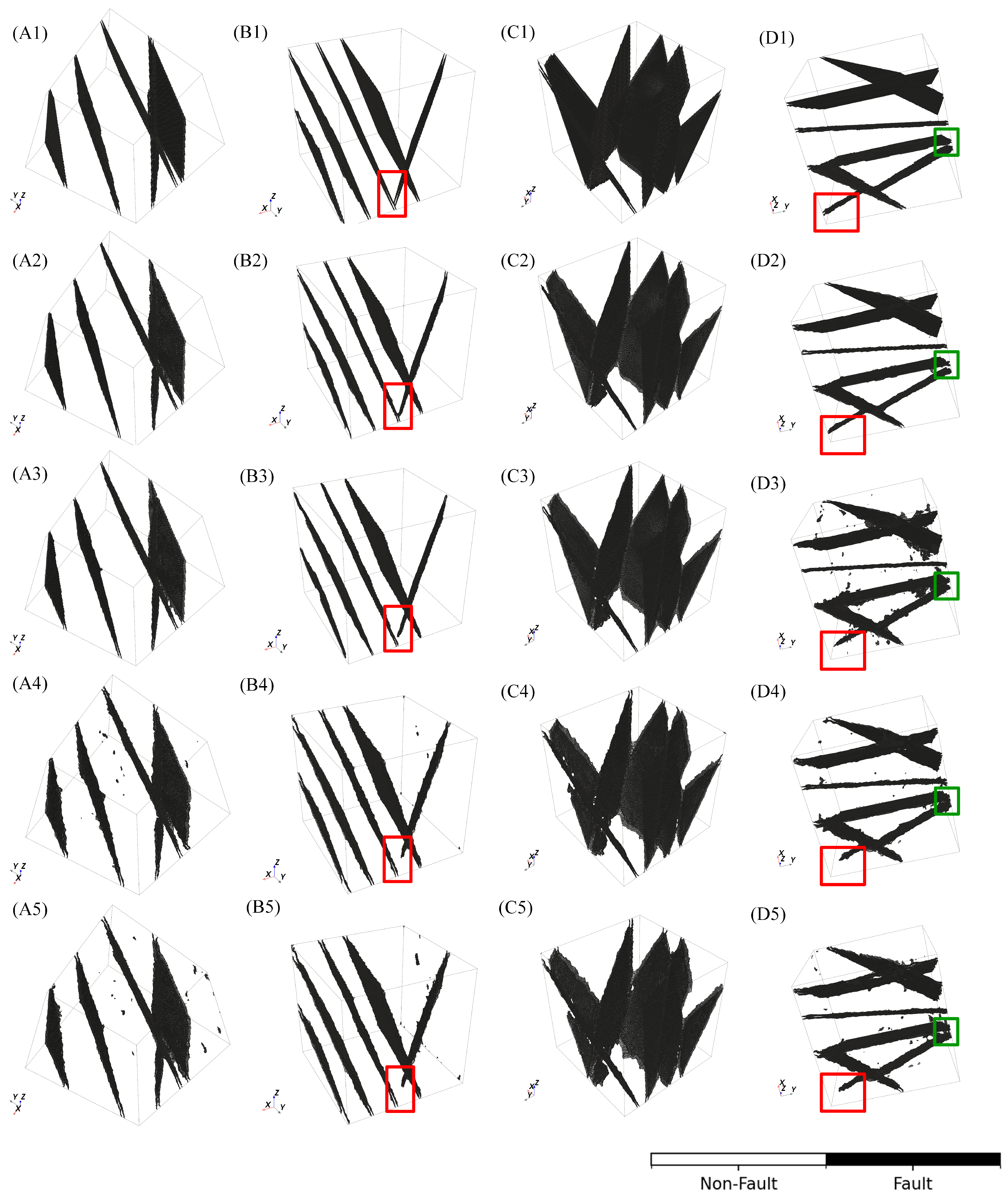
Building upon the comprehensive multi-dimensional quantitative evaluation presented above, this research further conducted qualitative visualization analysis to more intuitively elucidate the performance disparities among different networks in terms of fault identification details. Four 3D seismic data samples were randomly selected from the validation set. Their predicted results by the proposed SwiftSeis-AWNet network (
Figure 10(A2–D2)) and three comparative networks—TransUNet (
Figure 10(A3–D3)), FaultSeg3D (
Figure 10(A4–D4)), and ResUNet (
Figure 10(A5–D5))—were visualized in 3D. The comprehensive visualization is presented in
Figure 10, with the first row (
Figure 10(A1–D1)) showing the corresponding ground truth fault labels.
Overall, the visual comparison in
Figure 10 strongly corroborates the quantitative findings in
Table 2. The SwiftSeis-AWNet network consistently demonstrates exceptional identification performance across all four samples. Its predicted fault systems not only exhibit high fidelity to the ground truth fault labels at a macroscopic structural framework level but also excel in preserving the geometric continuity of fault surfaces, delineating intricate fracture networks, and identifying subtle, small-scale discontinuities. Notably, the network exhibits superior noise robustness.
In contrast, predictions from FaultSeg3D and ResUNet commonly suffer from more pronounced fault fragmentation, blurred boundaries, and a significant presence of high-frequency noise voxels—either surrounding the fault zones or scattered throughout the background. These visually manifest as isolated high-amplitude points or irregular patchy artifacts, severely compromising the structural integrity of the interpreted fault system and the reliability of geological interpretation. While the TransUNet network demonstrates relatively robust performance and a more complete main fault structure in samples A to C, it reveals insufficient adaptability to specific complex geological conditions in Sample D (
Figure 10(D3)). This manifests as numerous fine, geologically meaningless, discrete predicted points, creating artifacts that impede accurate interpretation of the primary fault structures.
Specific highlighted regions within
Figure 10 further underscore SwiftSeis-AWNet’s precise identification capabilities. For instance, in the red bounding boxes, our proposed network accurately captures subtle geological features such as fault tips, branching intersections, and minute geometric variations along fault surface edges. This ensures both the sharpness of fault boundaries and the fidelity of their geometric morphology, effectively mitigating common issues observed in other networks, such as eroded fault boundaries, sudden displacement variations due to excessive smoothing, or the loss of small-scale en-echelon array details. Crucially, in the ground truth label of Sample D (
Figure 10(D1)), the green bounding box highlights two spatially very proximate fault surfaces. SwiftSeis-AWNet (
Figure 10(D2)) successfully delineates these two independent structural units with clear separation, maintaining a distinct and identifiable inter-fault block. Furthermore, each fault surface maintains its complete morphology and excellent continuity, without exhibiting unreasonable fault fusion or artificial bridging phenomena.
4.4.2. F3 Dataset
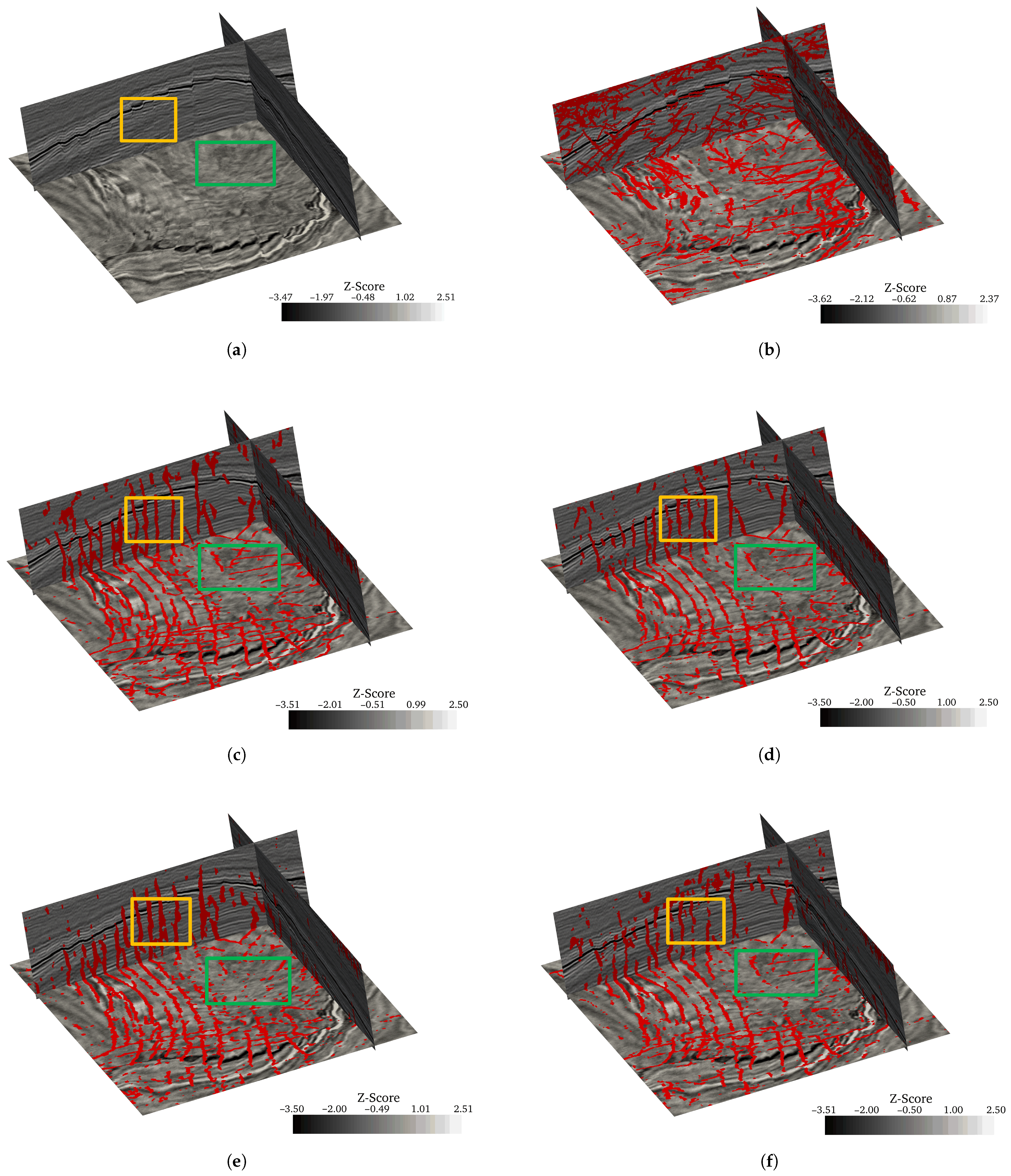
For a more intuitive evaluation of the proposed SwiftSeis-AWNet network’s performance in the 3D seismic fault detection task, comparative experiments were conducted using the aforementioned baseline networks on seismic data from a specific area within the F3 block of the Dutch North Sea. The results are visually presented in
Figure 11.
Figure 11 illustrates (a) a slice of the original seismic volume and (b) the fault response obtained using the traditional Ant Tracking algorithm. As observed in
Figure 11b, traditional methods, such as Ant Tracking, prove ineffective in capturing seismic faults. Particularly in low signal-to-noise ratio (SNR) areas, the identified fault information appears chaotic, making it challenging to effectively distinguish true fault structures. Moreover, this method is susceptible to interference from strong-amplitude, continuous formation reflections, often leading to the misidentification of formation boundaries as faults and consequently, low reliability in the identified fault interpretations.
Focusing on the area highlighted by the yellow box, which exhibits a series of nearly vertical, densely developed faults, the proposed network (
Figure 11c) successfully identified these faults, presenting clear, sharp fault surface responses with excellent vertical continuity. These results accurately reflect the offset relationships of the seismic reflections (horizons) visible in the original data (
Figure 11a). In contrast, FaultSeg3D (
Figure 11d) exhibits significant discontinuity in fault tracing within this area, with prediction results appearing as numerous short, fragmented segments that fail to effectively connect and form complete fault surfaces. The identification result of TransUNet (
Figure 11e), while capturing the main fault trends, reveals relatively blurred fault surfaces. Furthermore, some adjacent faults exhibit a ‘sticking’ or ‘merging’ phenomenon, indicating insufficient spatial resolution. The ResUNet-based network (
Figure 11f) demonstrates the poorest performance in this area, with its fault identification results appearing extremely fragmented, rendering effective structural interpretations almost impossible.
The area highlighted by the green box represents a more complex geological structure, characterized by low-dip, relatively weak-response faults or structural deformation zones. In this area, the original data (
Figure 11a) clearly shows the bending and discontinuity of seismic reflections (horizons). The proposed network (
Figure 11c) continues to perform excellently, reliably tracing these dipping, low-SNR fracture features. The identified fault network structure is coherent and highly consistent with the geological expectations. Conversely, FaultSeg3D (
Figure 11d) exhibits poor fault continuity in this area, often missing many subtle fractures. The identification results from TransUNet (
Figure 11e) and ResUNet (
Figure 11f) in this area are similarly unsatisfactory, presenting numerous scattered, geologically insignificant isolated points or short segments that fail to effectively delineate the structural framework.
4.4.3. Kerry Dataset
To evaluate the network’s capability in identifying more elusive and intricate fracture systems within field data, our approach was tested on the New Zealand Kerry 3D seismic dataset. Specifically, a sub-volume characterized by abundant faults, covering inline range 100–196, crossline range 200–712, and time samples 80–400 ms, was utilized for this assessment.
This dataset is particularly challenging, as it comprises a unique class of geologically present faults with atypical geophysical responses—specifically, fracture surfaces that have formed without significant vertical or horizontal displacement of the strata on either side (as highlighted by the green circle in
Figure 12). These “no-displacement faults” pose a formidable challenge to traditional identification methods that primarily rely on the principle of seismic horizon offset.
Mainstream deep learning networks, including FaultSeg3D (
Figure 12d), TransUNet (
Figure 12e), and ResUNet (
Figure 12f), alongside traditional ant-tracking algorithms (
Figure 12b), uniformly failed to effectively delineate these crucial geological structures. This is primarily because the feature extraction and fusion mechanisms within these networks or algorithms tend to prioritize strong amplitude contrasts and pronounced geometric offsets associated with macroscopic fractures. Consequently, they often interpret these subtle discontinuity signals as mere background noise or stratigraphic variations, leading to significant information omission.
It is important to note that the field seismic datasets utilized in this section, namely the F3 and Kerry block, do not have publicly available, ground-truth fault annotations. Consequently, a direct quantitative evaluation using metrics such as the Dice coefficient is not feasible. While new manual annotations could be created, they would introduce a significant degree of interpreter-dependent subjectivity. Therefore, to ensure a robust and objective assessment, we adopted a comparative qualitative analysis framework, a standard and accepted practice in seismic interpretation under such circumstances. The performance of all models, including our proposed method and the baselines, was systematically evaluated against a consistent set of geologically driven criteria: (1) fault continuity and coherence, (2) boundary sharpness, and (3) overall structural plausibility against the seismic reflectors. This approach allows for a rigorous relative assessment of performance, establishing which model produces the most geologically meaningful and interpretable results.
In contrast, the proposed SwiftSeis-AWNet network, leveraging its attention mechanism, dynamically assesses and weights feature information across diverse scales. This capability enables it to acutely capture subtle seismic waveform response changes directly attributable to the rock fracturing itself, independent of any accompanying stratigraphic displacement. Even in the absence of macroscopic displacement, this module can discern spatially continuous, subtle patterns associated with fracture surfaces within multi-scale feature maps and assign them higher weights during the feature fusion process. Consequently, the network not only successfully identified this challenging fault but also delineated its surface with remarkable clarity and continuity, distinctly differentiating it from the surrounding geological background. This comparative experiment powerfully validates SwiftSeis-AWNet’s unique advantages in fine structural analysis, particularly its substantial potential in identifying early-stage, subtle, or atypical fracture architectures.
4.5. Ablation Experiments
To precisely quantify the contribution of the proposed AWSDI module and evaluate its effectiveness within the SwiftSeis-AWNet architecture for 3D seismic fault identification, an extensive ablation research was designed and conducted in this section. This research aims to isolate and validate the crucial role of the AWSDI module by comparatively analyzing the impact of different feature fusion strategies on overall network performance.
We systematically compared the performance of three network configurations on the same test dataset using common quantitative indices, including Accuracy, Precision, Recall, IoU, Dice Coefficient, and Loss Function Value, alongside three structural integrity indices. The detailed quantitative evaluation results are presented in
Table 3.
A comprehensive analysis of the experimental results leads to the following key conclusions: The negligible performance difference between the original and our simplified MedNeXt empirically validates that our architectural streamlining effectively reduces complexity without a significant trade-off in representational power. The SwiftSeis-AWNet network consistently demonstrated optimal performance across all evaluation indices. It not only achieved the highest values in traditional indices measuring voxel-level segmentation accuracy and possessed the lowest loss function value but also led in structural indices reflecting geological structure fidelity: securing the highest FCS and the lowest ASSD and 95th Percentile HD95.The results from SwiftSeis-AWNet and Simplified MedNeXt + SDI underscore the pivotal role of the attention-weighted mechanism. A clear performance degradation across all indices was observed when AWSDI was replaced with the attention-free SDI module. This unequivocally confirms that the attention mechanism effectively optimizes the multi-scale feature fusion process, not only enhancing pixel-level prediction accuracy but also critically improving the continuity and geometric precision of the predicted fault structures. Furthermore, the comparison between Simplified MedNeXt + SDI and the baseline Simplified MedNeXt highlights the necessity of a dedicated multi-scale fusion module over simple feature merging. Simplified MedNeXt + SDI consistently outperformed the baseline network, which relies on element-wise addition for fusion, across all evaluated indices. This demonstrates that, compared to basic skip-connection fusion methods, designing specialized multi-scale feature injection and fusion mechanisms is essential for enhancing both voxel-level accuracy and structural preservation in fault identification.
To provide visual corroboration for the quantitative ablation results, this study presents a qualitative comparison on representative slices from the F3 and Kerry datasets (
Figure 13 and
Figure 14). Comparing the original MedNeXt (c) with our Simplified MedNeXt (d), this study observed no significant degradation in fault identification, confirming that our backbone simplification effectively reduces complexity without compromising core performance. The introduction of the SDI module (e) substantially suppresses the background noise and artifacts present in the baseline result (d). Finally, the addition of our AWSDI module in SwiftSeis-AWNet (f) not only retains this noise robustness but also markedly enhances the sharpness and continuity of fine fault details, which appear smoother and less defined in the SDI-only version (e).
5. Discussion
The experimental results presented in this study demonstrate that our proposed SwiftSeis-AWNet achieves state-of-the-art performance in 3D seismic fault identification, consistently outperforming established baseline models across both quantitative metrics and qualitative geological plausibility. This success stems from a synergistic combination of a lightweight, domain-adapted backbone architecture and a novel, attention-driven feature fusion mechanism. In the following sections, we will delve deeper into the key aspects of our methodology, discussing the rationale behind our architectural design choices, the implications of our findings for industrial-scale applications, and the inherent limitations of the current study that pave the way for future research.
5.1. Rationale for Architectural Design Choices
The selection of the expansion ratio R within our network’s inverted residual blocks is a critical design choice that directly mediates the balance between model expressiveness and computational complexity. In this study, R was uniformly set to two, a decision informed by a comprehensive consideration of model efficiency, established design paradigms, and task-specific characteristics. Primarily, adhering to our core objective of constructing a “swift” and lightweight network, a conservative expansion ratio is a key strategy for managing the parameter count and computational load (FLOPs), which is crucial when processing large-scale 3D seismic volumes. Furthermore, this choice draws inspiration from the success of canonical efficient architectures like MobileNetV2 [
27], which have demonstrated that modest expansion factors can achieve an excellent trade-off between performance and efficiency. More importantly, for the specific task of fault identification, which involves recognizing geometrically structured features, an excessively high expansion ratio risks creating an “over-parameterized” model. Such a model may be prone to learning noise or irrelevant stratigraphic details from the data, rather than the essential structural characteristics of the faults themselves. Consequently, a moderate expansion ratio helps to instill an appropriate inductive bias in the model, mitigating overfitting and ultimately optimizing overall performance.
5.2. Basis of Model’s Generalization to Complex Faults
The model’s ability to learn and identify complex and subtle faults (such as the no-displacement faults discussed in
Section 4.4.3) is attributed to the following geological diversity contained within the synthetic volumes:
- (1)
Spatially Varying Displacements and “Quasi-Zero-Displacement” Zones: A key feature, as detailed by Wu et al. [
22], is that fault displacements are not constant but vary spatially, decreasing from a maximum at the fault’s center to zero at its edges and tips. This design is paramount, as it naturally creates a vast number of samples representing low-to-zero displacement regions. The seismic response in these zones mimics that of subtle, no-displacement fractures, characterized by faint waveform distortions, amplitude dimming, or phase discontinuities, rather than obvious reflector offsets. This provides the model with critical training examples for learning non-typical fault responses.
- (2)
Diversity in Fault Geometry and Morphology: The synthesis process incorporates a high degree of randomization in fault dip, strike, and morphology. This generates a wide array of fault types, from high-angle normal faults to complex networks involving intersections, splays, and en-echelon patterns. The fault thickness is also implicitly varied through the labeling process, where fault labels span two pixels adjacent to the fault plane. This comprehensive geometric diversity compels the model to learn a more generalized and robust representation of fault-related seismic textures, preventing it from relying on any single, idealized fault pattern.
5.3. Implications for Industrial-Scale Applications
Beyond academic metrics, the industrial viability of a deep learning model is determined by a holistic balance of accuracy, speed, and resource requirements. It is important to contextualize the “efficiency” of SwiftSeis-AWNet in this light. While its single-patch inference time may not be the absolute fastest among all tested models, its computational profile, characterized by a low parameter count and FLOPs, offers a distinct advantage in resource efficiency. A comparison with TransUNet, a high-performing baseline, illustrates this point: SwiftSeis-AWNet achieves comparable or superior accuracy while achieving a 22.4% reduction in inference time (predicting a 1283 volume in 93.8 ms compared to TransUNet’s 120.9 ms), with a reduction of approximately 98% in parameter count and FLOPs. This substantial improvement in resource efficiency translates into tangible industrial benefits. The significantly lower memory and computational footprint can reduce hardware costs and broaden access to advanced AI interpretation. For basin-scale surveys, this efficiency can enhance scalability and potentially accelerate overall project turnaround times. Furthermore, it makes interactive workflows more feasible, where an interpreter can rapidly iterate on the model. In essence, SwiftSeis-AWNet demonstrates a strong balance between achieving high accuracy and maintaining a high degree of computational and resource economy, positioning it as a practical and scalable solution for real-world industrial applications.
A pertinent consideration for any new method is its practical feasibility on large-scale industrial surveys, where data volumes often exceed the dimensions used during training. The architecture of SwiftSeis-AWNet allows for a degree of flexibility in input size. This was demonstrated in our application to the field datasets, where both the F3 and Kerry data volumes, which have dimensions different from the 1283 training cubes, were processed directly. However, for industrial-scale surveys measured in terabytes, processing the entire volume at once is generally infeasible due to universal GPU memory constraints. In such contexts, a standard patch-based processing workflow is employed. This procedure involves systematically dividing the large volume into smaller, overlapping 3D patches of a manageable size (e.g., 1283 voxels). Each patch is then processed individually by the trained network. Finally, the resulting output patches are reassembled into a single, full-sized volume, with predictions in the overlapping regions blended to ensure a seamless result. The lightweight nature of SwiftSeis-AWNet, characterized by its low resource requirements per patch, makes this workflow highly efficient and scalable, positioning it as a practical solution for real-world industrial implementation.
The preceding discussions highlight that the strength of SwiftSeis-AWNet lies not in a single metric but in its synergistic performance across multiple dimensions. Our architectural choices have yielded a model that is not only accurate at the voxel level but also robust in preserving geological structures, efficient in its use of computational resources, and flexible enough for practical large-scale deployment. This holistic balance between precision, structural fidelity, and practical efficiency is what ultimately defines its value for real-world seismic interpretation challenges.
6. Conclusions
This research introduced SwiftSeis-AWNet, a novel deep learning framework specifically engineered to address the critical shortfalls of existing state-of-the-art AI methods in 3D seismic fault identification—namely, their insufficient edge precision and poor noise robustness. The framework is built upon an optimized MedNeXt backbone, enhanced by integrating a SDI module. Critically, to overcome information loss in the SDI module, we designed the innovative AWSDI module. This core contribution uses a dynamic weighting mechanism to adaptively fuse multi-scale features, directly confronting the aforementioned challenges.
Comprehensive evaluations confirmed the superiority of our approach. On a public synthetic dataset, SwiftSeis-AWNet outperformed mainstream models like ResUNet, FaultSeg3D, and TransUNet, not only in traditional voxel-level metrics but also in advanced geological structure indices (FCS, ASSD, HD95), which validated its enhanced ability to preserve fault continuity and geometric fidelity. Furthermore, generalization tests on the F3 and Kerry field datasets demonstrated its practical utility, yielding interpretations that were demonstrably sharper and more structurally coherent than those from both traditional algorithms and competing deep learning models. Ablation studies decisively verified that the AWSDI module is the key driver of these improvements, enhancing sensitivity to subtle fractures and overall result clarity.
However, we acknowledge the limitations of this study. While SwiftSeis-AWNet shows strong resilience to Gaussian noise, its performance against other noise types remains to be quantified. It is also important to clarify the implication of our model’s lightweight nature. While its low parameter count and FLOPs do not necessarily guarantee the absolute fastest single-patch inference time, they signify a crucial advantage in deployment agility and resource efficiency. Our model achieves a superior balance of accuracy and macro-level efficiency with significantly lower resource consumption, making advanced AI-powered interpretation more accessible. Moreover, the model’s generalization capabilities, while promising, require further validation across a wider spectrum of complex geological settings. Future work will focus on incorporating multi-modal seismic attributes to improve geological interpretability and exploring self-supervised learning to mitigate the dependency on large annotated datasets.


