1. Introduction
Human motion analysis is central to various fields, including physical rehabilitation, human–robot interaction, biomechanical research, and health monitoring [
1,
2,
3,
4]. The ability to quantify movement patterns and joint kinematics provides essential information for designing adaptive systems, assessing recovery, and developing personalized interventions [
5]. In particular, the estimation of upper limb joint angles is a key metric in evaluating motor function in clinical and real-world environments [
6]. These measurements support the development of robotic assistance, prosthetic control, and rehabilitation tools that rely on biomechanical feedback to function effectively. At the same time, wearable technologies have enabled real-time tracking of physiological and kinematic variables in naturalistic settings. Recent developments include smart textiles for respiration monitoring [
7], open-source smartwatches for physical activity and heart rate tracking [
8], and medical health patches that provide continuous cardiorespiratory data using dry electrodes [
9], illustrating the growing potential of wearable systems in integrated health assessment.
Traditionally, optical motion capture systems (e.g., Vicon
®, OptiTrack
®) have been used as the gold standard for obtaining ground-truth joint angles due to their sub-millimeter spatial accuracy [
10]. However, these systems require fixed infrastructures, extensive camera calibration, and controlled laboratory conditions, making them impractical for deployment in everyday environments. Their spatial requirements and sensitivity to marker occlusion further limit accessibility outside research facilities [
11].
In response to these limitations, IMUs have gained popularity as wearable alternatives for motion capture [
12]. These low-power sensors infer segment orientation and joint angles across diverse conditions. Despite their advantages in portability and ease of integration, conventional IMU-based approaches often rely on dense sensor configurations (typically 7–10 units), which can present several challenges. These include:
Sensor-to-segment misalignment, which can introduce substantial errors in joint angle estimation. Fan et al. reported errors exceeding 24° in the knee when misalignment exceeded 15°, highlighting the sensitivity of such systems to mounting orientation errors [
13].
Inter-sensor drift during prolonged recordings, especially in dynamic movements such as running, where orientation accuracy deteriorates over time without correction mechanisms [
14].
Although IMUs are generally rated as comfortable by users, especially when embedded in clothing or mounted non-invasively, increasing the number of sensors can complicate setup and maintenance, affecting overall usability in natural environments.
These limitations motivate the development of minimal-sensor configurations, where a reduced number of strategically placed IMUs can still deliver high-accuracy joint angle estimates through robust modeling techniques [
15].
1.1. Deep Learning and Reduced Sensor Approaches
The integration of deep learning into motion estimation enables direct mapping from raw IMU data to joint kinematics. Recurrent neural networks (RNNs), particularly LSTM and CNN-LSTM hybrids, capture temporal dependencies critical for dynamic joint angle estimation. These models compensate for sparse inputs by learning latent biomechanical relationships [
16,
17].
Recent studies confirm that minimal IMU configurations can achieve accuracy comparable to optical systems when combined with optimized deep learning architectures. For example:
Kim et al. introduced the Activity-in-the-loop Kinematics Estimator (AIL-KE), an end-to-end CNN-LSTM model using only two IMUs (wrist and chest). By integrating activity classification into the pipeline, they achieved shoulder joint angle errors under 6.5°—a 17 % improvement over a baseline without behavioral context [
18]. However, this approach is primarily aimed at analyzing activities with periodic behaviors.
Alemayoh et al. showed that a single IMU placed on the shank or thigh can estimate lower-limb joint angles with a mean absolute error of 3.65° using a BLSTM, demonstrating feasibility for sagittal-plane kinematics during walking [
15]. No upper limbs were analyzed in this study.
Airaksinen et al. systematically assessed trade-offs in IMU configurations and concluded that the minimal configuration with acceptable classifier performance includes at least a combination of one upper and one lower extremity sensor [
19].
1.2. Problem Statement: Toward Practical and Scalable Joint Angle Estimation
Despite the growing interest in IMU-based motion tracking, achieving accurate upper limb joint angle estimation under real-world constraints remains an open challenge. Optical motion capture systems offer exceptional precision but are limited by their dependence on controlled environments. In contrast, wearable IMU solutions enable free-living monitoring but often rely on dense sensor networks that compromise usability [
20].
The need for scalable and user-friendly solutions calls for approaches that maintain high accuracy while minimizing hardware complexity. Reducing the number of IMUs requires robust neural learning frameworks capable of extracting informative representations from partial data streams. This trade-off between model complexity, number of sensors, and system deployability remains a challenge. Reducing sensor count reduces observability, but intelligent modeling strategies can compensate for this loss. Evaluating different neural architectures under constrained input conditions is essential to identify scalable and efficient solutions [
21].
1.3. Proposed Framework
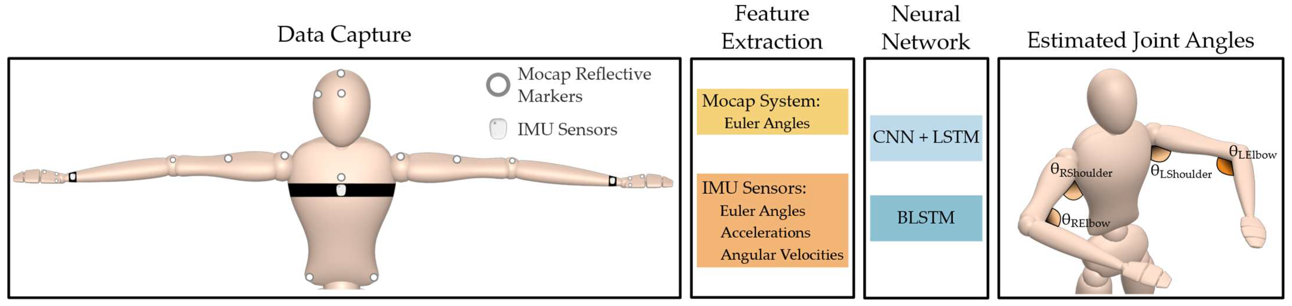
To address these challenges, this work proposes a deep learning framework that estimates upper limb joint angles using only three IMUs located at the chest and wrists. This configuration ensures biomechanical relevance while minimizing invasiveness. We assessed the effectiveness of two different model architectures: a CNN-LSTM, which uses convolutional layers to extract spatial features followed by temporal modeling, and a Bidirectional LSTM (BLSTM), which processes sequences in both forward and backward directions to enhance context awareness. An overview of the proposed sensor placement and model pipeline is illustrated in
Figure 1.
The models were trained using IMU data synchronized with ground truth MoCap measurements, allowing the system to learn joint-specific motion patterns. By comparing both architectures, we evaluated the trade-offs between inference, accuracy, and temporal smoothness.
1.4. Contributions and Paper Organization
This work contributes to the ongoing effort to simplify joint angle estimation systems for practical deployment in health and rehabilitation contexts. We demonstrate that with a minimal sensor configuration and proper model selection, it is possible to achieve high-accuracy estimation of upper limb kinematics.
The rest of the paper is structured as follows:
Section 2 describes the dataset acquisition, sensor placement, and preprocessing steps.
Section 3 introduces the model architectures and training procedure.
Section 4 presents quantitative results comparing CNN-LSTM and BLSTM under specific motion conditions.
Section 5 discusses the implications of these findings, highlights current limitations, and outlines future research directions toward scalable, real-world biomechanical monitoring systems.
2. Materials and Methods
2.1. Instrumentation
This study employed a dual-system configuration comprising an IMU-based wearable platform and an optical MoCap system to obtain synchronized kinematic datasets. The IMU system utilized MetaMotionS devices developed by Mbientlab Inc. (San Jose, CA, USA), capable of capturing raw linear acceleration, angular velocity, and orientation in quaternion or Euler-angle format. These sensors operate over Bluetooth Low Energy (BLE) and provide onboard fusion capabilities for orientation estimation.
For ground-truth kinematics, an OptiTrack
® motion capture system (OptiTrack, Corvallis, OR, USA) was used in conjunction with Motive software (version 3.3.0.1), which handled the digitization and recording of all OptiTrack
® data. This system computes segmental joint angles based on 3D marker trajectories and predefined biomechanical models. All data streams were timestamped and synchronized to ensure alignment between IMU and MoCap recordings. Although MoCap systems are considered the gold standard, they are not free from limitations such as marker displacement and soft tissue artifacts. To address these, a previous study conducted by the authors evaluated the feasibility of emulating an IMU sensor using a MoCap system by performing specific controlled movements across and along each coordinate axis, as well as combined motions [
22]. The results demonstrated high consistency between the motion capture output and expected IMU behavior, supporting the reliability of MoCap-based ground truth for this application.
2.2. Data Acquisition
A single 10 min recording session was performed by a single subject, involving continuous upper limb movements executed at a natural speed and full range of motion. Prior authorization from the Institutional Review Board (IRB) was obtained to perform this study. The shoulder joint was evaluated across three degrees of freedom: abduction/adduction, flexion/extension, and internal/external rotation. The elbow joint was evaluated only in flexion/extension. No segmentation or repetition scheme was enforced, ensuring a representative sequence of natural motion.
IMU data were collected at 50 Hz and included tri-axial acceleration, angular velocity, and quaternion orientation. This sampling rate was selected based on prior studies indicating that 50 Hz is sufficient to capture the natural frequency of human motion without aliasing, even during fast transitions [
23,
24]. All quaternion data were converted to Euler angles using a ZYX intrinsic rotation convention. This conversion was necessary due to the limitations of directly using quaternions in neural network training.
Euler angles offer scalar orientation values aligned with anatomical axes, making them more interpretable for both biomechanical analysis and neural network learning. Unlike quaternions, which are abstract and non-intuitive, Euler angles correspond directly to clinically meaningful joint motions such as flexion or rotation. This alignment facilitates better feature learning and promotes faster convergence during model training, as the network can associate specific signal patterns with anatomically relevant movements. The dataset is available in the following reference [
25].
2.3. Experimental Design
All data collection was conducted by a single subject under consistent environmental conditions. More subjects will be included for future studies to account for other body sizes, limbs, and dynamics. The subject wore three IMUs placed on the chest and both wrists, along with reflective markers positioned according to the standardized upper-limb marker set required by the Motive skeletal solver (See
Figure 1). The OptiTrack
® system consisted of 7 infrared cameras surrounding the capture volume to provide high-fidelity 3D tracking.
Figure 2 illustrates the complete setup used during data collection.
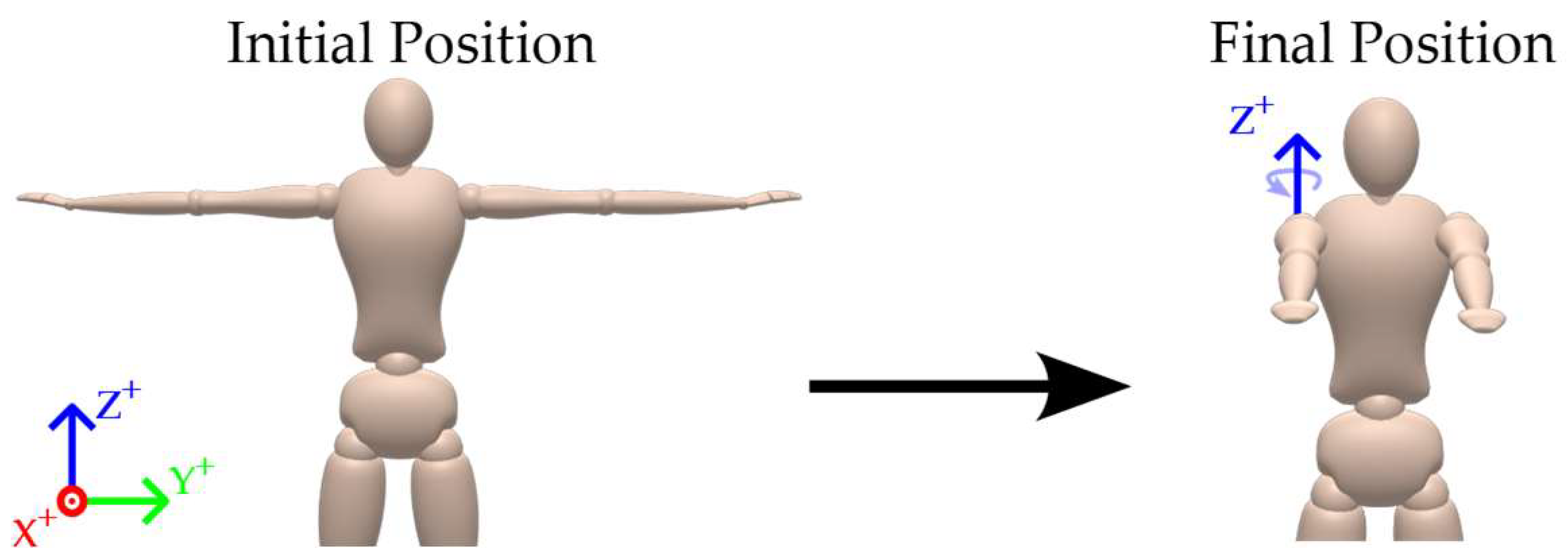
At the beginning of each recording session, the subject adopted a T-pose posture, with both arms extended horizontally and palms facing downward. This standardized position served as the initial reference for all subsequent movements and was used to align the coordinate systems of the IMU and MoCap data. Starting from a well-defined T-pose ensured consistent orientation across both systems and facilitated the synchronization of reference frames during post-processing.
Following this posture, the subject performed a series of continuous upper limb motions at a natural speed and amplitude. These movements included:
A shoulder rotation around the
Z-axis (Yaw), shown in
Figure 3.
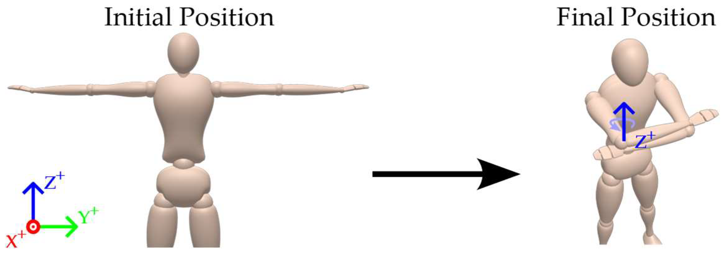
A shoulder flexion/extension around the
X-axis (Roll), shown in
Figure 4.
An elbow flexion/extension primarily around the
Z-axis (Yaw), shown in
Figure 5.
The sequence was designed to reflect a broad range of typical daily activities, ensuring sufficient variability across all rotational degrees of freedom to support robust model training.
Ground-truth joint angles were obtained from the OptiTrack® motion capture system using Motive’s embedded biomechanical solver. This software computed shoulder and elbow joint angles based on the 3D trajectories of the reflective markers. The resulting time series of joint angles served as the reference targets for training and evaluating the proposed learning models.
2.4. Data Preprocessing
The raw data acquired from the wearable sensors consisted of acceleration, angular velocity, and quaternion signals from each IMU. Static angles were initially captured in quaternion format because the sensor fusion algorithm implemented in the Mbientlab MetaMotionRL devices (version r0.5) with firmware-enabled 9-axis sensor fusion, yields more accurate orientation estimates when the data is exported directly in this format. In contrast, exporting orientation directly as Euler angles from the device introduced noticeable inaccuracies. Therefore, the data was first collected in quaternion form and subsequently converted into Euler angles for model training. Preliminary experiments using quaternions as training targets yielded poor results, since the networks struggled to preserve the unit norm required for valid quaternions, and their abstract 4D representation limited the model’s ability to learn meaningful geometric relationships. Euler angles provided a more interpretable and effective representation for the estimation task.
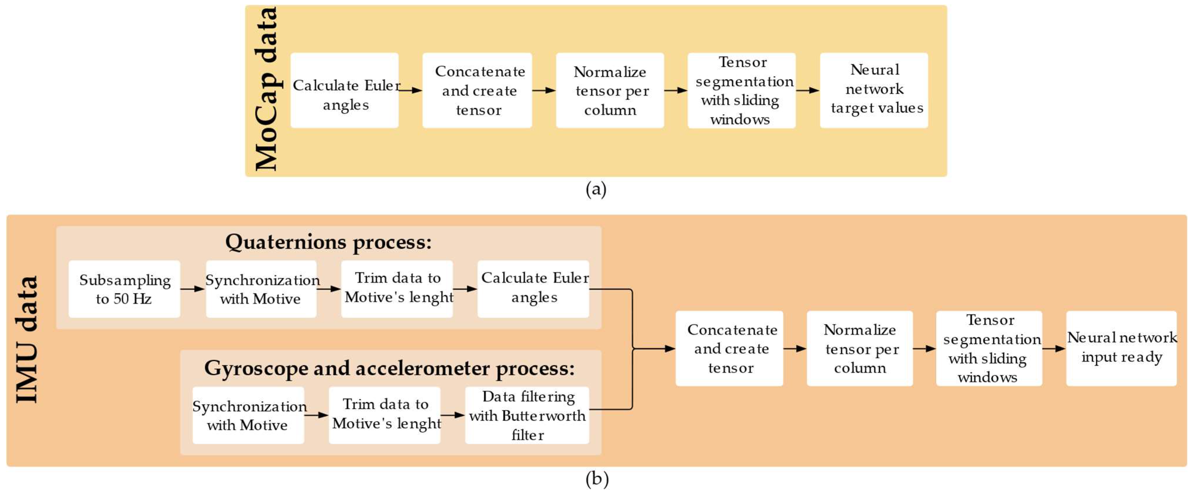
To prepare this data for use in neural network models, a structured and multi-stage preprocessing pipeline was developed, encompassing data synchronization, trimming, subsampling, segmentation into temporal windows, and normalization. This pipeline is illustrated in
Figure 6.
2.4.1. Type of Measured Data
Each IMU sensor recorded triaxial accelerometer data (g), gyroscope data (°/s), and quaternion orientation data (W, X, Y, Z). A separate CSV file was generated for each signal type and each sensor.
2.4.2. Synchronization and Trimming
Data acquisition was initiated first with the three IMU sensors. After a 5 s delay to ensure all sensors were actively recording, the MoCap system was started. This approach ensured that the MoCap system provided a consistent and precise timestamp reference to align all IMU data streams. During preprocessing, the IMU files were temporally synchronized by aligning their internal timestamps to the MoCap start time. Once synchronization was achieved, all data streams were trimmed to match the duration recorded by the MoCap system. Since the OptiTrack® Motive software allows configuration of a fixed trial duration, this ensured all signals were aligned and had identical length. Notably, IMU recorded a few extra seconds at the end due to delayed manual stopping; trimming ensured these were discarded, resulting in consistent frame alignment across all devices.
2.4.3. Subsampling
Mbientlab sensors record quaternions at a fixed sampling rate of 100 Hz, while accelerometer and gyroscope data were configured to operate at 50 Hz. Additionally, the OptiTrack® motion capture system provided ground-truth joint angles sampled at 50 Hz. To ensure temporal consistency across all input and target signals, quaternion data were subsampled to 50 Hz by retaining every other sample.
2.4.4. Filtering
A low-pass Butterworth filter (fifth-order, cutoff frequency = 5 Hz) was applied to the accelerometer and gyroscope data to attenuate high-frequency noise. This cutoff frequency was selected to preserve the dominant frequencies associated with voluntary human limb motion, which typically fall below 6 Hz [
26]. In biomechanics, low-pass filtering is commonly applied to both kinematic and kinetic data to improve signal quality and reduce noise. Common cutoff frequencies range from 3 to 10 Hz [
27], with 6 Hz often used as a representative value, as seen in tools like OpenSim [
27,
28]. The filter was implemented using the filtfilt function to achieve zero-phase distortion. Quaternion data were not filtered.
2.4.5. Tensor Preparation and Normalization
The recordings were loaded and concatenated into a unified dataset. The input features included yaw, pitch, and roll (transformed Euler angles from quaternions), angular velocities (ωx, ωy, ωz), and linear accelerations (ax, ay, az) from each IMU sensor, resulting 27 columns across the chest, right wrist, and left wrist sensors. The output (target) variables were 10 joint angles derived from the MoCap system: 3 degrees of freedom (DOF) at each shoulder and 2 DOF at each elbow.
Min–max normalization was applied independently to the input and output variables using the MinMaxScaler from scikit-learn. The scaler was fitted on the training data and reused to normalize the validation data and later to inverse-transform the model outputs during evaluation.
2.4.6. Sliding Window Design
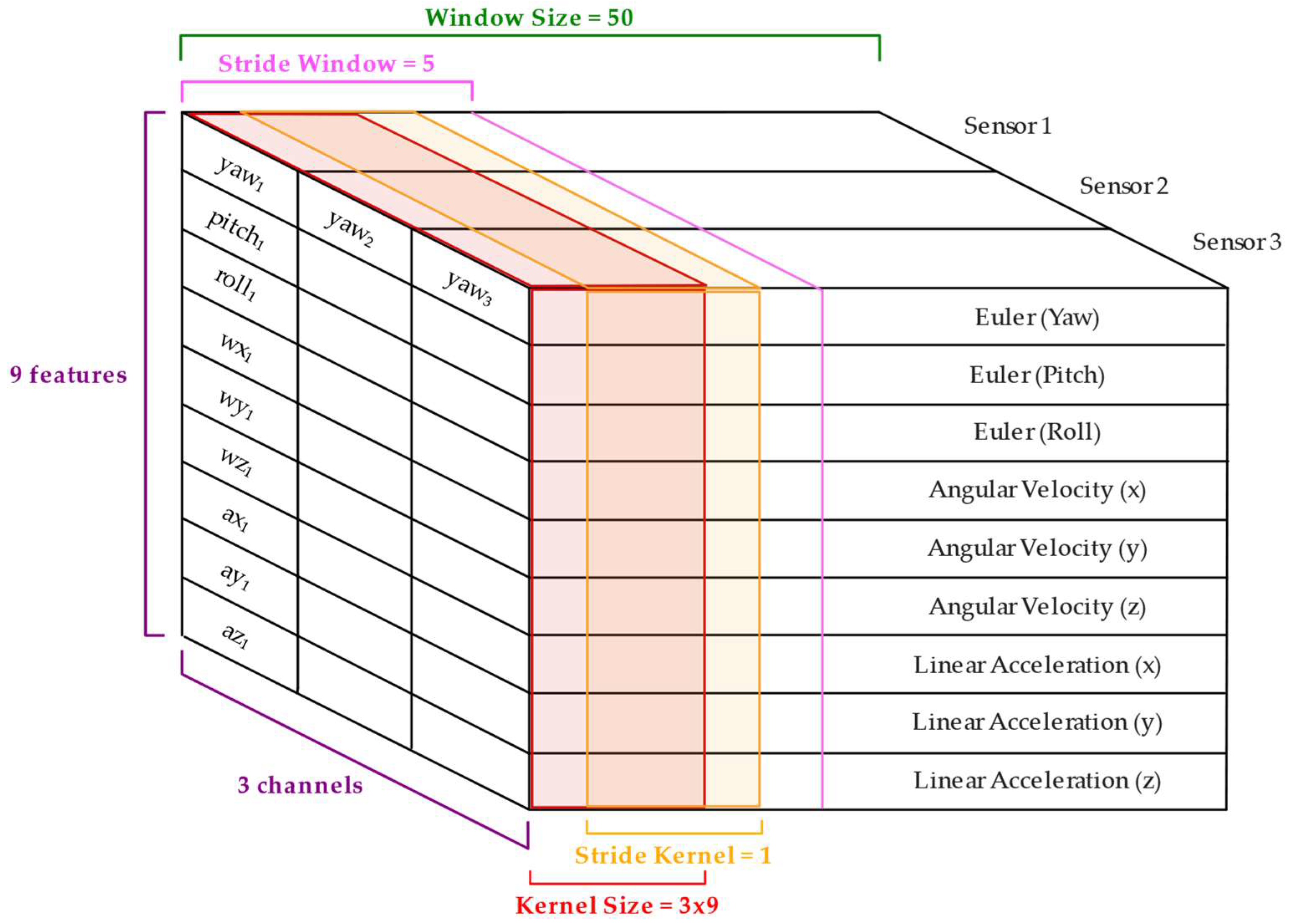
The normalized data were segmented into overlapping temporal windows of 50 frames (corresponding to 1 s of data at 50 Hz) using a stride of 5 frames as shown in
Figure 7. This configuration results in a 90% overlap between consecutive windows, ensuring high temporal continuity across samples. The high overlap also helps preserve dynamic changes between windows, particularly important in short sequences where rapid joint movements occur. This decision was especially beneficial given the reduced number of sensors and the system’s low observability, as it increased the number of training samples and improved the model’s ability to capture sequential dependencies and postural transitions. While lower overlaps (e.g., 50% and 25%) were tested and yielded acceptable and poor results, respectively, 90% consistently led to better performance. Overall, this setting promoted generalization and mitigated overfitting by exposing the model to more nuanced motion patterns.
Following the windowing step, the output tensors were trimmed to compensate for the shift introduced by the convolutional operations within the CNN-LSTM architecture. This alignment guaranteed consistency between the sequence length of the inputs and the targets. A detailed explanation of this architectural adjustment is presented in
Section 2.5.
2.4.7. Data Split
After preprocessing and tensor construction, the data was divided into training and validation sets. Five of the six available recordings were used for training, while the other one was exclusively reserved for validation. This take-independent split ensured that the validation set contained motion patterns not directly seen during training, allowing for a more realistic assessment of the model’s generalization ability. The resulting split produced approximately 30,000 training frames and 6000 validation frames after windowing.
With the dataset structured for training and validation, the next step involved designing and evaluating neural network architectures capable of learning the complex relationship between the multivariate inertial inputs and the corresponding joint angles. Two deep learning models were assessed for this task: a CNN-LSTM network and a BLSTM network.
2.5. Comparative Analysis of Architectures
The CNN-LSTM and BLSTM architectures were assessed to estimate upper limb joint angles from inertial data; however, they differ in structure, computational complexity, and learning dynamics, which impact their respective advantages and limitations.
The CNN-LSTM model leverages convolutional layers to extract local spatiotemporal features from segmented IMU signals before passing them to the LSTM layers. This hierarchical structure enables effective encoding of short-term dynamics and reduces the dimensionality of the input prior to sequential modeling. Its use of 2D convolution allows for localized feature learning across both sensor modalities and time, promoting generalization while keeping the model relatively lightweight. Moreover, the presence of a CNN front-end introduces a degree of robustness to noise and spatiality, helping the model focus on motion-relevant features [
29]. However, the choice of kernel size and stride introduces a shape mismatch between input and output sequences, requiring architectural adjustments and additional processing steps such as target cropping.
In contrast, the BLSTM model eliminates the need for convolutional preprocessing by directly operating on a flattened representation of the IMU signals. Its bidirectional nature allows it to access both past and future motion trends within the input window, enabling potentially more accurate estimation in temporally ambiguous situations [
30]. This ability to integrate broader temporal context may improve performance in scenarios with delayed responses or nonlinear movement transitions. However, the absence of a CNN component also means that the model may be more sensitive to noise or irrelevant features, as it lacks an explicit mechanism for spatial feature extraction.
Overall, while the CNN-LSTM model offers a more compact and interpretable architecture that balances performance with computational efficiency, the BLSTM provides richer temporal modeling capabilities that may prove advantageous in tasks requiring higher sensitivity to motion context.
2.6. Neural Network Architectures
The selection of architectural parameters, such as the number of layers, kernel size, and hidden units, was selected based on related works and optimized through manual configuration adjustments validated experimentally. Several configurations were tested iteratively, adjusting hyperparameters such as filter size, dropout rate, and the number of recurrent layers until stable convergence and low validation error were achieved. These decisions were also informed by related works in joint angle estimation using IMUs. The following subsections describe the final architectures and training strategies adopted for each model.
2.6.1. Convolutional-Long Short-Term Memory (CNN-LSTM) Architecture
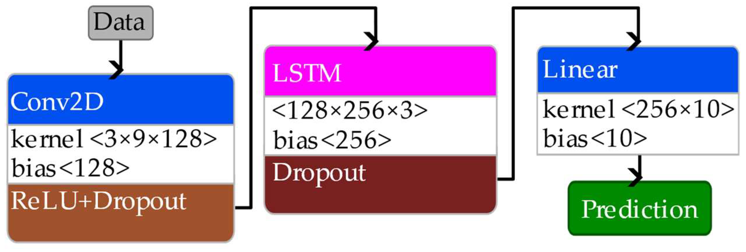
The model input consisted of 50-frame temporal windows. For each sensor, nine features were included: three Euler angles, three angular velocities, and three linear accelerations, resulting in a total of 27 features per frame. Each input sample was thus represented as a tensor of shape (50, 27), which was expanded to (1, 50, 27) to comply with the input requirements of 2D convolutional layers. The overall structure of the CNN-LSTM architecture is shown in
Figure 8.
The first layer of the network was a 2D convolutional layer with 128 filters and a kernel size of (3, 10), applied without padding. This kernel spanned three timesteps and ten feature dimensions, enabling the model to extract spatiotemporal correlations across the time and all sensors. Due to the convolution operation, the time dimension was reduced from 50 to 48 frames. To maintain consistency between input and target sequences, the ground truth joint angle series was trimmed by two frames during preprocessing, as mentioned in the previous section.
Following the convolutional layer, a dropout layer with a rate of 0.3 was used to mitigate overfitting by randomly deactivating neurons during training. The output of the convolutional stage was reshaped from (batch, 64, 48, 1) to (batch, 48, 64), making it suitable for input to a recurrent layer.
To capture the temporal dynamics of the motion, the network employed a single LSTM layer with 256 hidden neurons. This layer processed the sequential features extracted by CNN and learned temporal dependencies across the 48-frame sequence. The output of the LSTM at each timestep was passed to a fully connected layer that mapped the 256-dimensional hidden state to 10 outputs per frame, representing the joint angles of interest. The target labels for the neural networks correspond to the joint angles at the final frame of each shifting window. This strategy is consistent with established practices in the literature, where the output label is aligned with the last timestep of the input sequence, ensuring temporal consistency between the observed inertial dynamics and the predicted joint angles [
15].
The target angles correspond to the rotational components (Yaw, Pitch, and Roll) of the shoulder and (Yaw and Pitch) of the elbow, for both left and right arms. This results in a total of 10 predicted joint angles per window, representing the angular orientation of each joint in the anatomical frame with respect to the initial T-pose posture.
The network was trained for 150 epochs using the Adam optimizer with a learning rate of 1 × 10⁻⁵. A batch size of 50 was used, matching the temporal length of each input window. The loss function employed was the Mean Absolute Error (MAE), selected for its interpretability in degrees and its robustness to outliers compared to squared-error-based metrics. Its exclusive use in this study ensured a simple and consistent evaluation framework across models and joints, prioritizing clarity and interpretability over the inclusion of multiple statistical indicators.
To prevent overfitting, a dropout rate of 30% was applied between layers, and early stopping was implemented during training based on the validation loss. This training strategy enabled the model to gradually minimize the angular discrepancy between predicted and ground-truth joint angles across all degrees of freedom.
2.6.2. Bidirectional Long Short-Term Memory (BLSTM)
To assess the impact of temporal context on angle estimation, an alternative architecture was implemented using a BLSTM network. Unlike the LSTM, which only captures dependencies in the forward temporal direction, the BLSTM processes the input sequence in both forward and backward directions simultaneously. This dual traversal allows the network to access past and future context at each timestep, which can be particularly beneficial when the prediction depends on motion trends occurring before and after a given frame.
In contrast to the CNN-LSTM model, the BLSTM architecture does not include convolutional layers; thus, the input tensor is not four-dimensional. Instead, the IMU data are directly reshaped into a three-dimensional tensor of shape (batch, window size, features), where the features dimension results from concatenating all sensor channels (i.e., acceleration, angular velocity, and Euler angles) across all devices, yielding an input tensor of shape (batch, 50, 27). This flattened representation preserves the temporal structure of the signal while providing the network with simultaneous access to all sensor signals. The overall structure of the CNN-LSTM architecture is shown in
Figure 9.
The BLSTM was composed of five stacked bidirectional LSTM layers, each with 512 hidden units per direction. Due to the bidirectional nature of architecture, the resulting hidden state dimension was 1024 (512 forward + 512 backward). The output of the final timestep was passed through a dropout layer (p = 0.3) and subsequently to a fully connected layer that mapped the 1024-dimensional hidden representation to the 10 target joint angles.
This model was trained under the same conditions as the CNN-LSTM architecture: 150 epochs, a batch size of 50, and the Adam optimizer with a learning rate of 1 × 10⁻⁵. The Mean Absolute Error (MAE) was also used as the loss function to maintain consistency in evaluation. As with the CNN-LSTM model, a 30% dropout rate was introduced between layers, and early stopping was employed based on the validation loss to mitigate overfitting. This consistent training configuration facilitated a fair comparison between both architectures.
While the BLSTM adds complexity and computational cost compared to its unidirectional counterpart, its ability to incorporate future motion context into each prediction may enhance generalization in scenarios with temporally ambiguous or noisy input sequences. This trade-off between temporal context and model efficiency is further explored in the discussion section through a comparative analysis of results.
3. Results
To evaluate the performance of both neural network architectures, the validation was carried out using a sequence not seen during training. As described in
Section 2.3, this recording included three specific upper limb movements:
A shoulder rotation around the Z-axis (Yaw).
A shoulder flexion/extension around the X-axis (Roll).
An elbow flexion/extension primarily in the Z-axis (Yaw).
3.1. CNN-LSTM
To evaluate the CNN-LSTM model, complete predictions for each of the three selected movements are shown alongside ground truth angles to illustrate the general behavior of the network.
Figure 10 shows the model’s predictions for the three movements mentioned previously for the CNN-LSTM. The presented CNN-LSTM model demonstrates robust performance in predicting joint angles using only wrist and chest sensor data, achieving consistent prediction accuracy across multiple degrees of freedom. For both upper limbs, the model exhibits high precision in estimating planar movements, with shoulder Pitch errors as low as 3.67° (left) and 3.77° (right), and Roll errors measuring 5.08° (left) and 4.88° (right). These results indicate adequate capability in capturing fundamental movement patterns with satisfactory accuracy. Rotational (Yaw) predictions show slightly higher but still adequate performance, with shoulder errors of 8.58° (left) and 9.12° (right), and elbow errors of 9.90° (left) and 9.98° (right), this is considered satisfactory given the complexity of rotational kinematics and the minimal sensor configuration. The consistent performance across both limbs demonstrates the model’s generalization capabilities. The close correspondence between predictions and ground truth throughout most movement phases highlights the effectiveness of the CNN-LSTM architecture in learning meaningful spatiotemporal relationships from limited distal sensor data. It is important to note the model’s ability to accurately reconstruct proximal joint angles without direct measurements from shoulders or elbows, showcasing advanced pattern recognition capabilities.
3.2. BLSTM
The BLSTM model was evaluated using the same validation sequence as the CNN-LSTM, allowing direct comparison under identical conditions.
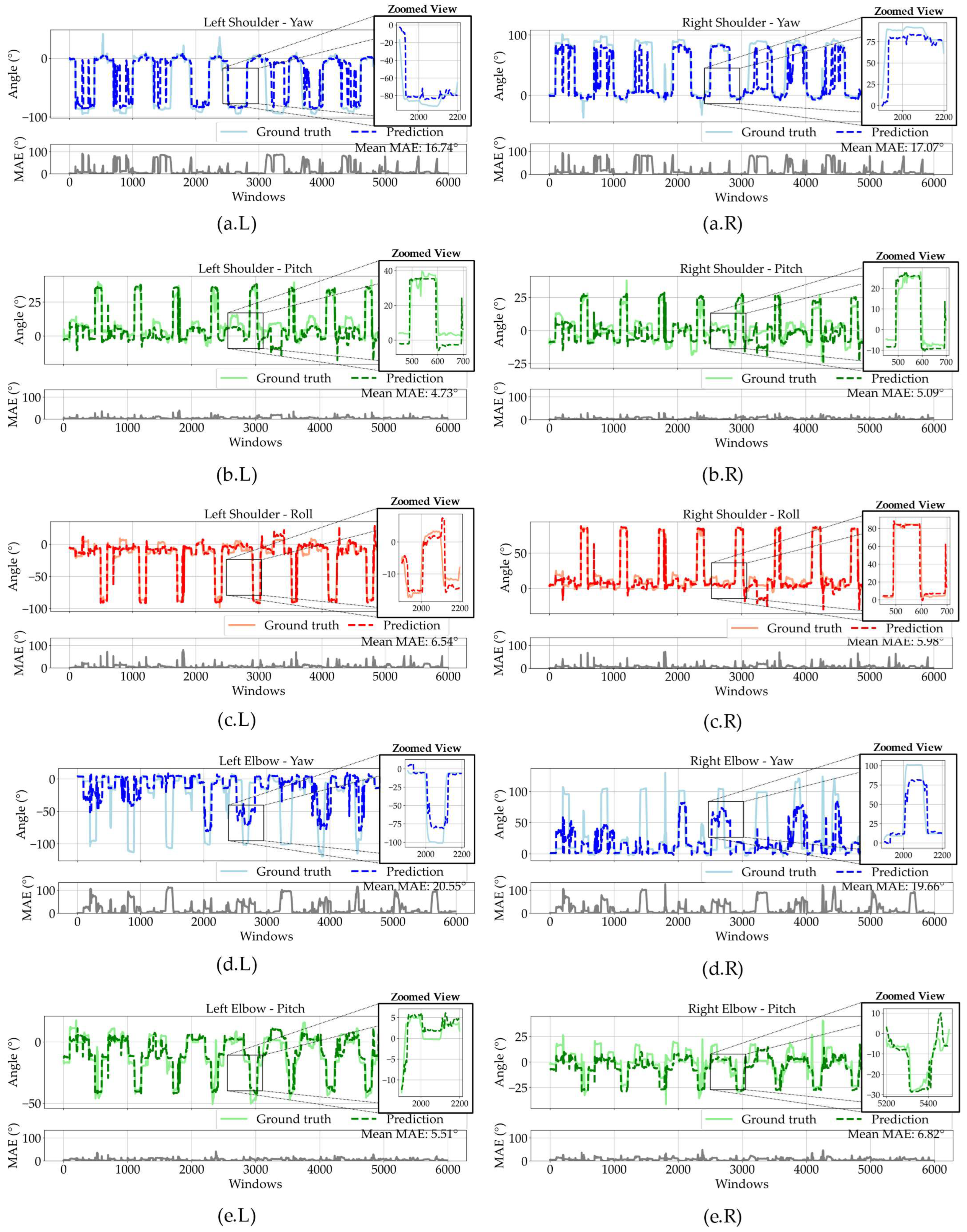
Figure 11 shows the model’s predictions for the three movements mentioned previously for the BLSTM. The BLSTM network demonstrates effective performance in predicting joint angles from limited sensor data, with particularly strong results for certain movement types. For the right shoulder, the model achieves acceptable accuracy in Pitch estimation (MAE: 5.09°) and maintains good performance for Roll movements (MAE: 5.98°). The elbow Pitch predictions also show competitive results with an MAE of 6.82°. While the Yaw predictions for both shoulder (MAE: 17.07°) and elbow (MAE: 19.66°) exhibit higher error values, these results remain significant given the inherent complexity of rotational kinematics and the minimal sensor configuration. The consistent performance across different joint angles highlights the model’s ability to capture fundamental movement patterns, with particularly accurate tracking of planar motions. The prediction curves closely follow the ground truth, highlighting the BLSTM’s ability to capture temporal dependencies. Notably, it reconstructs proximal joint angles using only wrist and chest sensors, demonstrating strong pattern recognition despite the limited sensor setup.
The CNN-LSTM model demonstrated strong performance in planar motion prediction, achieving MAEs of 3.67–5.08° for shoulder Pitch/Roll and 4.83–5.07° for elbow Pitch, while Yaw predictions yielded higher errors (8.58–9.98°). The BLSTM network showed comparable accuracy in planar movements, with shoulder Pitch/Roll MAEs of 5.09–5.98° and elbow Pitch at 6.82°, but exhibited increased Yaw prediction errors (17.07–19.66°). Both models successfully reconstructed joint angles using only wrist and chest data, with the CNN-LSTM showing slightly better overall precision, particularly in rotational (Yaw) estimations. The BLSTM maintained robust temporal tracking but displayed marginally higher deviations in complex rotations, suggesting differences in handling kinematic dependencies between architectures.
3.3. Architectures Computational Performance
To evaluate and compare the computational performance of the tested architectures, key metrics such as the number of parameters, model size, average inference time per batch and per sample, and GPU memory usage were measured.
Table 1 presents a side-by-side comparison between the CNN-LSTM and BLSTM models.
Both models were evaluated under the same conditions using a batch size of 50 and a window stride of 5 (90% overlap). The results show that the CNN-LSTM model is more computationally efficient than the BLSTM across all measured aspects. It required fewer parameters, occupied less storage, had faster inference times, and consumed less memory during execution.
4. Discussion and Future Work
The results from both the CNN-LSTM and BLSTM architectures demonstrate promising capabilities for joint angle prediction using minimal sensor configurations, with each showing distinct strengths. The CNN-LSTM achieved superior performance in planar movements (Pitch/Roll MAEs: 3.67–5.08°) and notably lower Yaw errors (8.58–9.98°) compared to the BLSTM (Pitch/Roll MAEs: 5.09–5.98°; Yaw: 17.07–19.66°). However, these higher Yaw errors can be attributed to the nature of sensor placement and the reduced observability of axial rotations in this configuration, which limits the detectable range and angular variation in the Yaw axis. Additionally, abrupt motion transitions involving rapid changes in velocity or acceleration were observed to be more error-prone, as such dynamic segments are more difficult for the models to capture, especially under reduced sensor input. Although no explicit segmentation by motion phase was performed, qualitative inspection of the predicted trajectories supports this observation.
On the other hand, the CNN-LSTM model demonstrated significantly better computational efficiency compared to the BLSTM. It required fewer parameters, reduced the model size, and lowered inference time and memory usage by a considerable margin. These differences reflect the higher complexity and resource demands of the BLSTM architecture. While BLSTM may offer benefits in modeling temporal dependencies due to its bidirectional structure, the CNN-LSTM achieved a better balance between computational cost and performance.
This suggests that the CNN-LSTM’s hybrid spatial-temporal feature extraction may better handle rotational kinematics. Both models effectively reconstructed proximal joint angles from distal sensors, validating their potential for wearable applications.
Future work will be focused on integrating lower limbs estimations and optimizing model architectures to combine the strengths of CNN-LSTM and BLSTM, potentially through hybrid designs or attention mechanisms, to further reduce errors in rotational axes. Architectural refinements could integrate CNN-LSTM’s spatial feature extraction with BLSTM’s bidirectional temporal modeling to further reduce Yaw errors. Targeted data augmentation, emphasizing rotational movements, could enhance generalization for both models. Additionally, addressing the current limitation of using a single subject, future validation will involve multi-subject datasets, including publicly available human activity recognition (HAR) datasets [
31] that capture a broader range of daily movements and inter-subject variability. Although upper limb motion generally exhibits lower variability across individuals compared to lower limb movements, techniques such as dropout and early stopping were applied during training to mitigate overfitting. To further enhance model robustness, transfer learning strategies could also be explored to adapt a pretrained model to new subjects, reducing the need for extensive retraining while mitigating subject-specific biases.
Hybrid approaches incorporating attention mechanisms and biomechanical constraints may improve rotational tracking. Attention could allow the model to assign greater weight to rotational components where errors are typically higher, enhancing its ability to focus on the most informative features. In parallel, introducing biomechanical constraints based on typical human joint ranges could guide the network toward more anatomically plausible predictions, acting as a form of regularization. Together, these strategies would support more accurate and consistent angle estimation, even under sensor limitations and diverse motion patterns. Sensor fusion techniques, such as sparse upper-body sensor integration, could be explored to disambiguate complex rotations while preserving wearability. The models’ complementary strengths also suggest potential for ensemble methods or adaptive switching between architectures based on motion complexity. In potential real-time applications, the CNN-LSTM architecture is more suitable due to its causal structure and lower computational demands. In contrast, BLSTM relies on future context, which limits its applicability in online scenarios; however, a short temporal buffer could be introduced to access limited future frames, enabling near real-time performance with minimal latency. Finally, validation should expand to diverse populations and real-time implementations to solidify its clinical and industrial applicability. These advancements would position such models as leading solutions for accurate, minimal-sensor motion capture across rehabilitation, sports science, and human–computer interaction.
5. Conclusions
This study demonstrates that deep learning architectures can effectively estimate upper-limb joint angles using only three IMUs placed on the chest and wrists, offering a practical alternative to multi-sensor or optical motion capture systems. The CNN-LSTM and BLSTM models both achieved competitive accuracy, with the CNN-LSTM excelling in precision for planar movements and complex rotations (Yaw), while the BLSTM provided smoother temporal predictions but exhibited higher errors in peak rotational estimations. These results validate the feasibility of minimal-sensor configurations for joint angle reconstruction, highlighting the CNN-LSTM’s superior spatial-temporal feature extraction and the BLSTM’s robust sequential modeling. The findings underscore the potential of such approaches to bridge the gap between laboratory-grade accuracy and real-world wearability, enabling applications in rehabilitation, sports science, and human–robot interaction.
Author Contributions
Conceptualization, K.N.-T. and J.F.P.-M.; methodology, K.N.-T., L.S.-A., J.L.R.-C. and J.F.P.-M.; software, K.N.-T.; validation, K.N.-T. and J.F.P.-M.; formal analysis, K.N.-T.; investigation, K.N.-T.; resources, J.F.P.-M.; data curation, K.N.-T.; writing—original draft preparation, K.N.-T.; writing—review and editing, K.N.-T., L.S.-A., J.L.R.-C. and J.F.P.-M.; visualization, K.N.-T.; supervision, J.F.P.-M.; project administration, J.F.P.-M.; funding acquisition, J.F.P.-M. All authors have read and agreed to the published version of the manuscript.
Funding
This research received financial support from the NSF EPSCoR Center for the Advancement of Wearable Technologies (CAWT) under Grant No. OIA-1849243.
Institutional Review Board Statement
The study was conducted under the Declaration of Helsinki and approved by the University of Puerto Rico’s Institutional Review Board (IRB) under protocol number 2024120022 (approved on 27 January 2025).
Informed Consent Statement
Informed consent was obtained from all subjects involved in the study.
Data Availability Statement
Conflicts of Interest
The authors declare no conflict of interest.
Abbreviations
The following abbreviations are used in this manuscript:
| IMU | Inertial Measurement Units |
| MoCap | Motion Capture |
| CNN | Convolutional Neural Network |
| LSTM | Long Short-Term Memory |
| BLSTM | Bidirectional Long Short-Term Memory |
References
- Aggarwal, J.K.; Cai, Q. Human Motion Analysis: A Review. Comput. Vis. Image Underst. 1999, 73, 428–440. [Google Scholar] [CrossRef]
- Choffin, Z.; Jeong, N.; Callihan, M.; Sazonov, E.; Jeong, S. Lower Body Joint Angle Prediction Using Machine Learning and Applied Biomechanical Inverse Dynamics. Sensors 2022, 23, 228. [Google Scholar] [CrossRef] [PubMed]
- Coker, J.; Chen, H.; Schall, M.C.; Gallagher, S.; Zabala, M. EMG and Joint Angle-Based Machine Learning to Predict Future Joint Angles at the Knee. Sensors 2021, 21, 3622. [Google Scholar] [CrossRef]
- Senanayake, D.; Halgamuge, S.; Ackland, D.C. Real-time conversion of inertial measurement unit data to ankle joint angles using deep neural networks. J. Biomech. 2021, 125, 110552. [Google Scholar] [CrossRef] [PubMed]
- Roggio, F.; Ravalli, S.; Maugeri, G.; Bianco, A.; Palma, A.; Di Rosa, M.; Musumeci, G. Technological advancements in the analysis of human motion and posture management through digital devices. World J. Orthop. 2021, 12, 467–484. [Google Scholar] [CrossRef]
- Höglund, G.; Grip, H.; Öhberg, F. The importance of inertial measurement unit placement in assessing upper limb motion. Med. Eng. Phys. 2021, 92, 1–9. [Google Scholar] [CrossRef]
- Cay, G.; Solanki, D.; Al Rumon, M.A.; Ravichandran, V.; Fapohunda, K.O.; Mankodiya, K. SolunumWear: A smart textile system for dynamic respiration monitoring across various postures. iScience 2024, 27, 110223. [Google Scholar] [CrossRef] [PubMed]
- Ravanelli, N.; Lefebvre, K.; Brough, A.; Paquette, S.; Lin, W. Validation of an Open-Source Smartwatch for Continuous Monitoring of Physical Activity and Heart Rate in Adults. Sensors 2025, 25, 2926. [Google Scholar] [CrossRef]
- Wei, J.C.J.; van den Broek, T.J.; van Baardewijk, J.U.; van Stokkum, R.; Kamstra, R.J.M.; Rikken, L.; Gijsbertse, K.; Uzunbajakava, N.E.; van den Brink, W.J. Validation and user experience of a dry electrode based Health Patch for heart rate and respiration rate monitoring. Sci. Rep. 2024, 14, 23098. [Google Scholar] [CrossRef]
- Aurand, A.M.; Dufour, J.S.; Marras, W.S. Accuracy map of an optical motion capture system with 42 or 21 cameras in a large measurement volume. J. Biomech. 2017, 58, 237–240. [Google Scholar] [CrossRef]
- Conconi, M.; Pompili, A.; Sancisi, N.; Parenti-Castelli, V. Quantification of the errors associated with marker occlusion in stereophotogrammetric systems and implications on gait analysis. J. Biomech. 2021, 114, 110162. [Google Scholar] [CrossRef] [PubMed]
- Zhao, J. A Review of Wearable IMU (Inertial-Measurement-Unit)-based Pose Estimation and Drift Reduction Technologies. J. Phys. Conf. Ser. 2018, 1087, 042003. [Google Scholar] [CrossRef]
- Fan, B.; Li, Q.; Tan, T.; Kang, P.; Shull, P.B. Effects of IMU Sensor-to-Segment Misalignment and Orientation Error on 3-D Knee Joint Angle Estimation. IEEE Sens. J. 2022, 22, 2543–2552. [Google Scholar] [CrossRef]
- Falbriard, M.; Meyer, F.; Mariani, B.; Millet, G.P.; Aminian, K. Drift-Free Foot Orientation Estimation in Running Using Wearable IMU. Front. Bioeng. Biotechnol. 2022, 8, 65. [Google Scholar] [CrossRef] [PubMed]
- Alemayoh, T.T.; Lee, J.H.; Okamoto, S. Leg-Joint Angle Estimation from a Single Inertial Sensor Attached to Various Lower-Body Links during Walking Motion. Appl. Sci. 2023, 13, 4794. [Google Scholar] [CrossRef]
- Hammerla, N.Y.; Halloran, S.; Ploetz, T. Deep, Convolutional, and Recurrent Models for Human Activity Recognition using Wearables. arXiv 2016. [Google Scholar] [CrossRef]
- Ordóñez, F.J.; Roggen, D. Deep convolutional and LSTM recurrent neural networks for multimodal wearable activity recognition. Sensors 2016, 16, 115. [Google Scholar] [CrossRef]
- Kim, D.; Jin, Y.; Cho, H.; Jones, T.; Zhou, Y.M.; Fadaie, A.; Popov, D.; Swaminathan, K.; Walsh, C.J. Learning-based 3D human kinematics estimation using behavioral constraints from activity classification. Nat. Commun. 2025, 16, 3454. [Google Scholar] [CrossRef]
- Airaksinen, M.; Räsänen, O.; Vanhatalo, S. Trade-Offs Between Simplifying Inertial Measurement Unit-Based Movement Recordings and the Attainability of Different Levels of Analyses: Systematic Assessment of Method Variations. JMIR Mhealth Uhealth 2025, 13, e58078. [Google Scholar] [CrossRef]
- Rast, F.M.; Labruyère, R. Systematic review on the application of wearable inertial sensors to quantify everyday life motor activity in people with mobility impairments. J. Neuroeng. Rehabil. 2020, 17, 148. [Google Scholar] [CrossRef]
- Mundt, M.; Johnson, W.R.; Potthast, W.; Markert, B.; Mian, A.; Alderson, J. A comparison of three neural network approaches for estimating joint angles and moments from inertial measurement units. Sensors 2021, 21, 4535. [Google Scholar] [CrossRef] [PubMed]
- Niño-Tejada, K.; Saldaña-Aristizábal, L.; Rivas-Caicedo, J.L.; Patarroyo-Montenegro, J.F. IMU Sensors Emulation using Motion Capture Systems. In Proceedings of the International Symposium on Intelligent Computing and Networking 2025, San Juan, Puerto Rico, 17–19 March 2025; Springer: Berlin/Heidelberg, Germany, 2025. [Google Scholar]
- Favata, A.; Gallart-Agut, R.; Pàmies-Vilà, R.; Torras, C.; Font-Llagunes, J.M. IMU-Based Systems for Upper-Limb Kinematic Analysis in Clinical Applications: A Systematic Review. IEEE Sens. J. 2024, 24, 28576–28594. [Google Scholar] [CrossRef]
- Pezenka, L.; Wirth, K. Reliability of a Low-Cost Inertial Measurement Unit (IMU) to Measure Punch and Kick Velocity. Sensors 2025, 25, 307. [Google Scholar] [CrossRef]
- Niño-Tejada, K.; Saldaña-Aristizabal, L.; Rivas-Caicedo, J.L.; Patarroyo-Montenegro, J.F. MoCap and IMU Dataset for Upper Limb Joint Angle Estimation. Zenodo 2025. [Google Scholar] [CrossRef]
- Winter, D.A. Biomechanics and Motor Control of Human Movement; Wiley: Hoboken, NJ, USA, 2009; Available online: https://books.google.com.pr/books?id=_bFHL08IWfwC (accessed on 10 June 2025).
- Crenna, F.; Rossi, G.B.; Berardengo, M. Filtering biomechanical signals in movement analysis. Sensors 2021, 21, 4580. [Google Scholar] [CrossRef]
- Yeo, S.S.; Park, G.Y. Accuracy verification of spatio-temporal and kinematic parameters for gait using inertial measurement unit system. Sensors 2020, 20, 1343. [Google Scholar] [CrossRef] [PubMed]
- Kasnesis, P.; Patrikakis, C.Z.; Venieris, I.S. PerceptionNet: A Deep Convolutional Neural Network for Late Sensor Fusion. In Intelligent Systems and Applications; Springer: Berlin/Heidelberg, Germany, 2018. [Google Scholar]
- Feigl, T.; Kram, S.; Woller, P.; Siddiqui, R.H.; Philippsen, M.; Mutschler, C. A bidirectional LSTM for estimating dynamic human velocities from a single IMU. In Proceedings of the 2019 International Conference on Indoor Positioning and Indoor Navigation IPIN, Pisa, Italy, 30 September 2019. [Google Scholar] [CrossRef]
- Rivas-Caicedo, J.L.; Saldaña-Aristizabal, L.; Niño-Tejada, K.; Patarroyo-Montenegro, J.F. Wearable IMU Sensor Dataset for Human Activity Recognition (HAR). Zenodo 2025. [Google Scholar] [CrossRef]
Figure 1.
Proposed framework for upper limb joint angle estimation using a reduced number of IMU sensors. Both CNN + LSTM and BLSTM were compared using the same dataset.
Figure 1.
Proposed framework for upper limb joint angle estimation using a reduced number of IMU sensors. Both CNN + LSTM and BLSTM were compared using the same dataset.
Figure 2.
Overview of the real-world setup used for experiments.
Figure 2.
Overview of the real-world setup used for experiments.
Figure 3.
Illustration of the shoulder yaw (Z-axis) movement performed during validation.
Figure 3.
Illustration of the shoulder yaw (Z-axis) movement performed during validation.
Figure 4.
Illustration of the shoulder roll (X-axis) movement performed during validation.
Figure 4.
Illustration of the shoulder roll (X-axis) movement performed during validation.
Figure 5.
Illustration of the elbow yaw (Z-axis) movement performed during validation.
Figure 5.
Illustration of the elbow yaw (Z-axis) movement performed during validation.
Figure 6.
Data preprocessing pipeline for the proposed framework. (a) Describes the processing of MoCap data used to generate the target joint angles for the neural networks. (b) Describes the processing of IMU signals.
Figure 6.
Data preprocessing pipeline for the proposed framework. (a) Describes the processing of MoCap data used to generate the target joint angles for the neural networks. (b) Describes the processing of IMU signals.
Figure 7.
Input tensor representation used in the CNN-LSTM architecture. The input consists of a window of 50 and 9 features per sensor, including Euler angles, angular velocities, and linear accelerations.
Figure 7.
Input tensor representation used in the CNN-LSTM architecture. The input consists of a window of 50 and 9 features per sensor, including Euler angles, angular velocities, and linear accelerations.
Figure 8.
Architecture of CNN-LSTM regression model.
Figure 8.
Architecture of CNN-LSTM regression model.
Figure 9.
Architecture of the BLSTM regression model.
Figure 9.
Architecture of the BLSTM regression model.
Figure 10.
CNN-LSTM full prediction for the left (L) and right (R) arm. (a.R/L) Shoulder Yaw, (b.R/L) Shoulder Roll, (c.R/L) Shoulder Pitch, (d.R/L) Elbow Yaw, (e.R/L) Elbow Pitch. Each sub-figure shows a zoomed view of the side of the transition and the MAE at the corresponding bottom.
Figure 10.
CNN-LSTM full prediction for the left (L) and right (R) arm. (a.R/L) Shoulder Yaw, (b.R/L) Shoulder Roll, (c.R/L) Shoulder Pitch, (d.R/L) Elbow Yaw, (e.R/L) Elbow Pitch. Each sub-figure shows a zoomed view of the side of the transition and the MAE at the corresponding bottom.
Figure 11.
BLSTM full prediction for the left (L) and right (R) arm. (a.R/L) Shoulder Yaw, (b.R/L) Shoulder Roll, (c.R/L) Shoulder Pitch, (d.R/L) Elbow Yaw, (e.R/L) Elbow Pitch. Each sub-figure shows a zoomed view of the side of the transition and the MAE at the corresponding bottom.
Figure 11.
BLSTM full prediction for the left (L) and right (R) arm. (a.R/L) Shoulder Yaw, (b.R/L) Shoulder Roll, (c.R/L) Shoulder Pitch, (d.R/L) Elbow Yaw, (e.R/L) Elbow Pitch. Each sub-figure shows a zoomed view of the side of the transition and the MAE at the corresponding bottom.
Table 1.
Computational performance comparison between CNN-LSTM and BLSTM.
Table 1.
Computational performance comparison between CNN-LSTM and BLSTM.
| Metric | CNN-LSTM | BLSTM |
|---|
| Total Parameters | 1,461,002 | 27,424,778 |
| Model Size (MB) | 5.58 | 104.62 |
| Avg. Inference time per batch (ms) | 15.894 | 43.456 |
| Avg. Inference time per sample (ms) | 0.318 | 0.869 |
| Max GPU memory used (MB) | 166.21 | 1122.33 |
| Disclaimer/Publisher’s Note: The statements, opinions and data contained in all publications are solely those of the individual author(s) and contributor(s) and not of MDPI and/or the editor(s). MDPI and/or the editor(s) disclaim responsibility for any injury to people or property resulting from any ideas, methods, instructions or products referred to in the content. |
© 2025 by the authors. Licensee MDPI, Basel, Switzerland. This article is an open access article distributed under the terms and conditions of the Creative Commons Attribution (CC BY) license (https://creativecommons.org/licenses/by/4.0/).


 ,
, 


