Dual-Branch Network for Blind Quality Assessment of Stereoscopic Omnidirectional Images: A Spherical and Perceptual Feature Integration Approach

Abstract

Stereoscopic omnidirectional images (SOIs) have gained significant attention for their immersive viewing experience by providing binocular depth with panoramic scenes. However, evaluating their visual quality remains challenging due to its unique spherical geometry, binocular disparity, and viewing conditions. To address these challenges, this paper proposes a dual-branch deep learning framework that integrates spherical structural features and perceptual binocular cues to assess the quality of SOIs without reference. Specifically, the global branch leverages spherical convolutions to capture wide-range spatial distortions, while the local branch utilizes a binocular difference module based on discrete wavelet transform to extract depth-aware perceptual information. A feature complementarity module is introduced to fuse global and local representations for final quality prediction. Experimental evaluations on two public SOIQA datasets—NBU-SOID and SOLID—demonstrate that the proposed method achieves state-of-the-art performance, with PLCC/SROCC values of 0.926/0.918 and 0.918/0.891, respectively. These results validate the effectiveness and robustness of our approach in stereoscopic omnidirectional image quality assessment tasks.

1. Introduction

With the rapid popularization of virtual reality (VR) technology, omnidirectional images, as a crucial visual medium, have become increasingly prevalent in various VR-related applications [1]. By integrating depth perception, stereoscopic omnidirectional images (SOIs) further enhance the immersive experience, providing viewers with a more realistic visual experience [2]. However, the complex processing at each stage of the SOI system can inevitably lead to quality degradation, which negatively impacts the user’s visual experience. Additionally, viewing SOIs through head-mounted display (HMD) devices differs significantly from traditional video viewing, as users can actively explore the content by changing their viewpoint. This unique interaction introduces new challenges in quality assessment. Therefore, developing effective SOI quality assessment (SOIQA) methods is important for enhancing the VR viewing experience and ensuring high-quality immersive content [3].

Currently, in most SOI systems, the processing of omnidirectional content is performed in the equirectangular projection (ERP) [4] format. Although traditional two-dimensional image quality assessment (2D IQA) methods can be directly applied to evaluate the quality of SOI in ERP format [5], they fail to address the geometric distortion generated in ERP, which leads to poor performance. Therefore, a direct solution for applying 2D IQA to omnidirectional images is to bridge the gap between the 2D IQA method and omnidirectional content. For instance, spherical PSNR (S-PSNR) [6], Craster Parabolic Projection PSNR (CPP-PSNR) [7], and weighted spherical uniform PSNR (WS-PSNR) [8] are all modified for omnidirectional image quality assessment (OIQA) based on traditional 2D IQA methods. Furthermore, by establishing a relationship between the two-dimensional plane and the sphere, S-SSIM [9] has been proven effective in evaluating the quality of omnidirectional images. Compared to ERP, cube-map projection (CMP) [10] divides the omnidirectional image into six faces of a cube, introducing less geometric distortion. This projection provides an intuitive approximation of a real 360° scene. Thus, several methods are also proposed based on CMP format images. However, unlike traditional 2D images, omnidirectional images allow viewers to freely change their viewing direction to explore the entire scene, while the viewport can only display content within the watching window at a time. None of the above methods have taken this characteristic of omnidirectional images into account. This also leaves significant room for research on omnidirectional image quality assessment (OIQA) methods.

Binocular perception is a key characteristic of stereoscopic visual processing and plays a crucial role in both three-dimensional (3D) images and stereoscopic omnidirectional images (SOIs) [11]. Due to disparity between the images received by two eyes, the human visual system exhibits fusion, competition, or inhibition effects [12]. However, these complex perceptual characteristics cannot be fully modeled, leading to inaccuracies in existing stereoscopic image quality assessment methods. As a result, developing an efficient and reliable SOI quality assessment method remains a significant challenge. To address these challenges, this paper proposes a novel deep learning framework that integrates the perceptual characteristics of omnidirectional vision and 3D depth perception to extract meaningful quality features of SOIs. Specifically, the framework eliminates sampling distortion introduced during the conversion from 2D to spherical representation using spherical convolution [13], ensuring a more accurate global feature representation. Additionally, a binocular difference module is introduced in the viewport processing stage to effectively capture stereoscopic perceptual quality, enabling more precise SOI quality prediction. Finally, the quality score is obtained through a fusion module. In essence, the contributions of this work are as follows:

(1)

To establish an overall perception of the scene and comprehensively describe the characteristics of the spherical image, an end-to-end spherical convolutional neural network is designed to extract spherical features in the ERP format based on the coordinate transformation between equirectangular and spherical parameterizations.

(2)

To model binocular interaction in HVS, a cross-convolution module leveraging a discrete wavelet transform captures differences between left and right view features across frequency domains. Additionally, a frequency domain feature-adaptive module enhances binocular feature representation. By effectively integrating visual signals, the proposed method improves the perceptual consistency of omnidirectional images, enabling a more accurate and comprehensive quality assessment.

(3)

To combine the features of different latitudes of the local and the sphere, a feature complementarity module is designed to supplement and fuse the features of the two branches. Comprehensive experiments on two benchmark databases demonstrate that our quality assessment model achieves better performance than existing SOIQA methods.

The remainder of this paper is organized as follows. Section 2 briefly reviews the related work on SOIQA and elaborates on the motivation of this work. In Section 3, the proposed SOIQA algorithm is described in detail. Section 4 presents the experimental results and corresponding analyses. Finally, conclusions are drawn in Section 5.

2. Related Works

In this section, we first review the related work on omnidirectional image quality assessment and stereoscopic image quality assessment and then elaborate on the motivation of the proposed SOIQA method.

2.1. Omnidirectional Image Quality Assessment

For omnidirectional image quality assessment, it can be mainly divided into two categories, namely, sampling-based methods and perception-based methods. The sampling-based methods aim to solve the non-uniform sampling problem in omnidirectional images. The S-PSNR method [6] maps the pixels of the original and reconstructed ERP images to the sphere and calculates PSNR through uniform sampling points to reduce the impact of projection transformation on quality assessment and more accurately capture the spherical space quality characteristics of panoramic images. The CPP-PSNR method by Zakharchenko et al. [7] takes a different approach. It converts the panoramic image to the Craster parabolic projection plane to calculate PSNR to solve the problem of projection format mismatch. The WS-PSNR by Sun et al. [8] and the WS-SSIM by Zhou et al. [14] are calculated based on the ERP format with the sphere area ratio factor, considering different projection and adjusting and optimizing the quality calculation to adapt to the characteristics of different projection formats. However, the sampling-based methods have limitations in practical applications. When applied to different projections, the projection transformation causes geometric changes, which may significantly affect human visual perception. Moreover, there is a lack of in-depth analysis of visual perception. Only sampling and projection are considered from a mathematical and geometric perspective, resulting in low consistency with human perception.

On the other hand, the perception-based methods focus more on the perceptual mechanism of the human visual system to the omnidirectional images. Upenik et al. [15] incorporated visual attention into the traditional PSNR metric. The OIQA method based on deep learning proposed by Kim et al. [16] consists of a quality predictor and a human perception guidance component. This method can automatically extract deep features from the image, thus more accurately assessing the quality of panoramic images. Lim et al. [17] used the latent space and position features to predict the quality score of distorted images and then optimized the corresponding score through adversarial learning with human opinions. Xia et al. [18] explored the asymmetric mechanism in visual perception for panoramic image quality assessment. By using WS-PSNR weights for local binary patterns and statistical analysis, they extracted high- and low-frequency features, leveraging brain physiology insights to refine feature extraction and analysis. Yang et al. [19] incorporated the luminance masking effect of human vision and the latitude characteristics of ERP images for SOI quality assessment. They noted that visual perception of luminance is influenced by surrounding brightness rather than being absolute. Additionally, variations in ERP image latitude affect the information content and quality perception. By integrating these factors, their assessment aligns more closely with human visual perception. Sun et al. [10] transformed ERP images into six viewpoint images (CMP) and designed a multi-channel deep learning model for quality prediction. This approach better reflects actual viewing conditions, as users typically perceive only part of a panoramic image through the viewport. By converting ERP images into CMP and analyzing them accordingly, the method more accurately simulates user experience and enhances quality assessment. Zheng et al. [20] converted ERP images to segmented spherical projection (SSP) and incorporated visual saliency to assess perceptual quality. By analyzing different projection angles, they sought to better capture image quality characteristics and human perceptual factors. Croci et al. [21] utilized spherical Voronoi diagrams to divide panoramic images into multiple patches for more precise quality assessment. By analyzing each region separately and integrating their quality evaluations, this method provides a comprehensive assessment of the entire image.

2.2. Stereoscopic Image Quality Assessment

In the early stages of stereoscopic image quality assessment (SIQA), various approaches were explored. Gorley et al. [22] estimated quality by simply combining the left and right image scores predicted by 2D-IQA methods. You et al. [23] examined the performance of 2D-IQA in SIQA and analyzed the impact of disparity information. However, these methods overlooked binocular visual effects, limiting their accuracy to symmetrically distorted images while exhibiting significant prediction deviations for asymmetrically distorted ones. To address this, Chen et al. [24] introduced a ring view incorporating disparity and binocular visual characteristics, enhancing assessment accuracy. Jiang et al. [25] applied non-negative matrix decomposition to learn monocular perception and color features, offering new insights for more precise SIQA. Liu et al. [26] proposed a synthetic ring view by fusing left and right perspectives, leveraging natural scene statistics (NSS) features to detect distortions and improve quality assessment through targeted feature extraction. In terms of visual stimulus definition, beyond fusing left and right viewpoints into a cyclopean image, quality can also be assessed through feature variations. For example, Bensalma et al. [27] simulated binocular signals generated by simple and complex cells to estimate binocular energy, forming a binocular energy quality index. Shao et al. [28] utilized sparse energy and sparse complexity for binocular combinations to derive a quality score. Geng et al. [29] extracted simple cell response features using independent component analysis, calculating feature similarity and local luminance consistency to measure structural and luminance distortions while incorporating feature energy and global relative luminance to model binocular fusion. Lin et al. [30] constructed cyclopean amplitude and phase maps based on binocular vision and local saliency, using a binocular space modulation function to weight feature similarity. Li et al. [31] developed a two-channel convolutional neural network (CNN) to simulate binocular fusion and competition for SIQA. Meng et al. [2] further integrated a visual cross model, a multi-scale information fusion model, and an attention model to simulate binocular fusion, designing an SIQA method accordingly.

2.3. Stereoscopic Omnidirectional Image Quality Assessment

The viewing experience of stereoscopic omnidirectional images (SOIs) is unique, typically facilitated by a head-mounted display (HMD) that provides a wider field of view with an immersive experience. This differs significantly from the viewing methods and perceptual characteristics of traditional 2D images, making conventional IQA methods unsuitable for SOIQA. To address this challenge, Chen et al. [32] processed SOIs as multiple viewport images and applied prediction coding theory, incorporating similarity and competitive advantage as 3D visual stimuli to aggregate viewport quality scores. Qi et al. [33] integrated viewport information, user behavior, and stereoscopic perception by combining a binocular perception model with an omnidirectional perception model, enabling no-reference viewport quality assessment. Zhou et al. [34] proposed a reference-based SOIQA framework adaptable to various projections by leveraging projection-invariant features and visual saliency. For deep learning-based approaches, Chai et al. [35] introduced a deformable convolutional network to model monocular–binocular interactions for blind quality assessment of stereoscopic panoramic images. This method extracts and analyzes image features through a specialized network structure, considering monocular–binocular interactions to enhance quality assessment. However, [35] does not account for the impact of user viewing behavior within the viewport on the final assessment. In summary, existing SOIQA methods still fail to fully consider key factors such as the viewport, user behavior, and stereoscopic perception. Additionally, most methods evaluate quality on a projection plane that does not align with the actual viewport, limiting their ability to accurately reflect user-perceived image quality.

2.4. Toward Perceptual SOIQA

Recent studies have highlighted several perceptual factors critical to immersive quality assessment. Attention-based mechanisms such as eye-tracking and saliency prediction have shown great potential in modeling user-perceived quality by identifying regions of interest within omnidirectional or VR content. These methods offer perceptual priors that can complement purely signal-based approaches. Additionally, video quality assessment (VQA) models introduce temporal dynamics, capturing motion consistency and flicker artifacts, which are essential for dynamic SOI or VR sequences. While our current work focuses on static SOIs, such temporal considerations are important for future extension to video-based SOIQA.

Moreover, some recent methods propose distortion-aware frameworks that adapt to different types or levels of degradation, either through multi-task learning or explicit distortion modeling. This adaptability is crucial for real-world applications with unknown or mixed distortions. Finally, perceptual asymmetry—especially in stereoscopic contexts—plays a vital role in subjective experience. Such studies show that differences in left and right view quality, as well as selective attention between hemispheres, can significantly affect quality perception, motivating future integration of asymmetric modeling into SOIQA systems.

In contrast to existing stereoscopic omnidirectional image quality assessment (SOIQA) methods which typically focus on 2D projections or fixed viewpoint patches, our method fully exploits the stereoscopic and spherical characteristics in a unified dual-branch architecture. Notably, some existing methods usually treat the left and right views separately, ignoring binocular interaction. Other existing methods are limited to viewport-based quality fusion without explicitly modeling binocular disparity or spherical distortion. In contrast, our model leverages spherical convolutions for geometry-aware representation and a binocular difference module (BDM) for perceptual disparity modeling, resulting in more robust and accurate quality predictions. Consequently, this paper proposes a dual-branch deep learning framework for SOIQA. To better align with human visual perception, spherical convolution is employed instead of traditional convolution, allowing for the preservation of more spatial information and maintaining the connectivity of the original spherical image. For viewport feature extraction, a binocular feature extraction network is designed that leverages binocular difference information and discrete wavelet transform (DWT) decomposition. This effectively captures the depth differences between the left and right images, enhancing stereoscopic perception. Furthermore, a global–local feature interaction network is introduced to model the mutual influence between the overall structure and fine details, capturing complex spatial relationships and further improving the accuracy of quality assessment.

3. Proposed Method

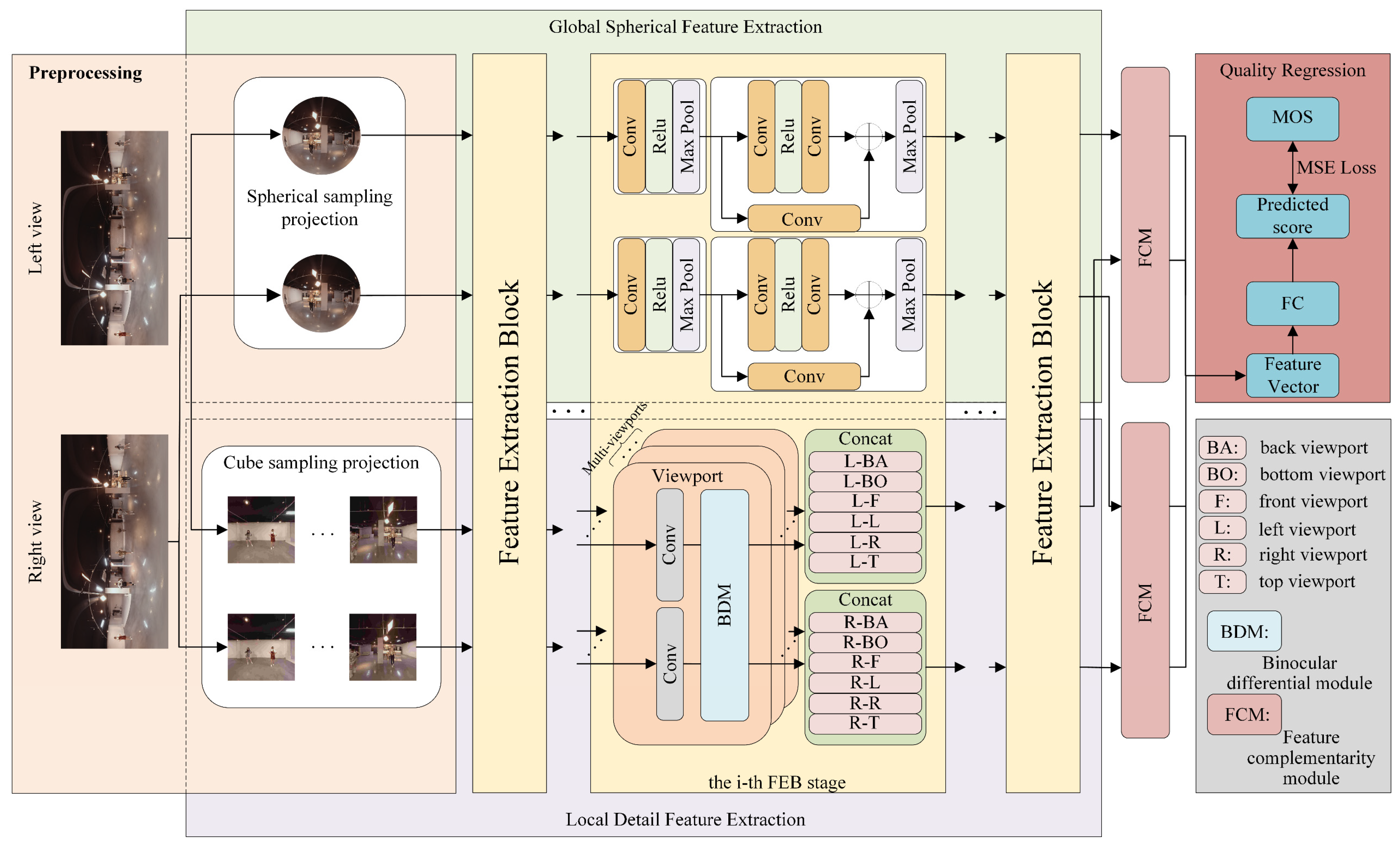
In this section, a detailed description of the proposed SOIQA method will be provided. The proposed method mainly consists of four components, namely, SOI preprocessing, global spherical feature extraction, local detail feature extraction, and overall quality regression. The overall architecture of the proposed framework is shown in Figure 1. It comprises four main components: (1) an SOI preprocessing module to generate different projection samples; (2) a global feature extraction branch based on spherical convolutions that models the structural distortion characteristics over the sphere; (3) a local feature extraction branch that captures perceptual and binocular cues via a binocular difference module (BDM) enhanced with frequency-aware representations; and (4) a feature complementarity module (FCM) that adaptively fuses global and local features to perform final quality regression. These components are designed to jointly capture both the geometry-specific and perception-specific properties of SOI distortions. The following sections provide a detailed explanation of each component.

3.1. SOI Preprocessing

Generally speaking, for omnidirectional images display, HMD devices first map the input ERP image into a sphere in three-dimensional spherical coordinates. Then, the device renders the visual content as a planar segment tangent to the sphere, determined by the viewing angle and field of view (FoV). By turning their heads, users can change their viewing angle, exploring the entire 360-degree image. Therefore, to comprehensively assess image quality, multiple viewpoints must be considered.

Inspired by this viewing procedure, we project the ERP image into both a spherical image and multiple viewport images. Specifically, six viewport images are rendered from a single omnidirectional image to ensure full coverage. Two views correspond to the poles, while the remaining four align with the horizon, rotating horizontally to encompass the equatorial region. The FoV is set to 90 degrees, consistent with most popular VR devices. Additionally, since users may begin viewing from different perspectives, our training samples include various viewpoints. The front view’s longitude is rotated from 0 to 360 degrees at intervals of ψ degrees, generating six viewport projections per ERP image. This approach not only expands the training set but also helps mitigate overfitting in deep learning models.

3.2. Global Spherical Feature Extraction

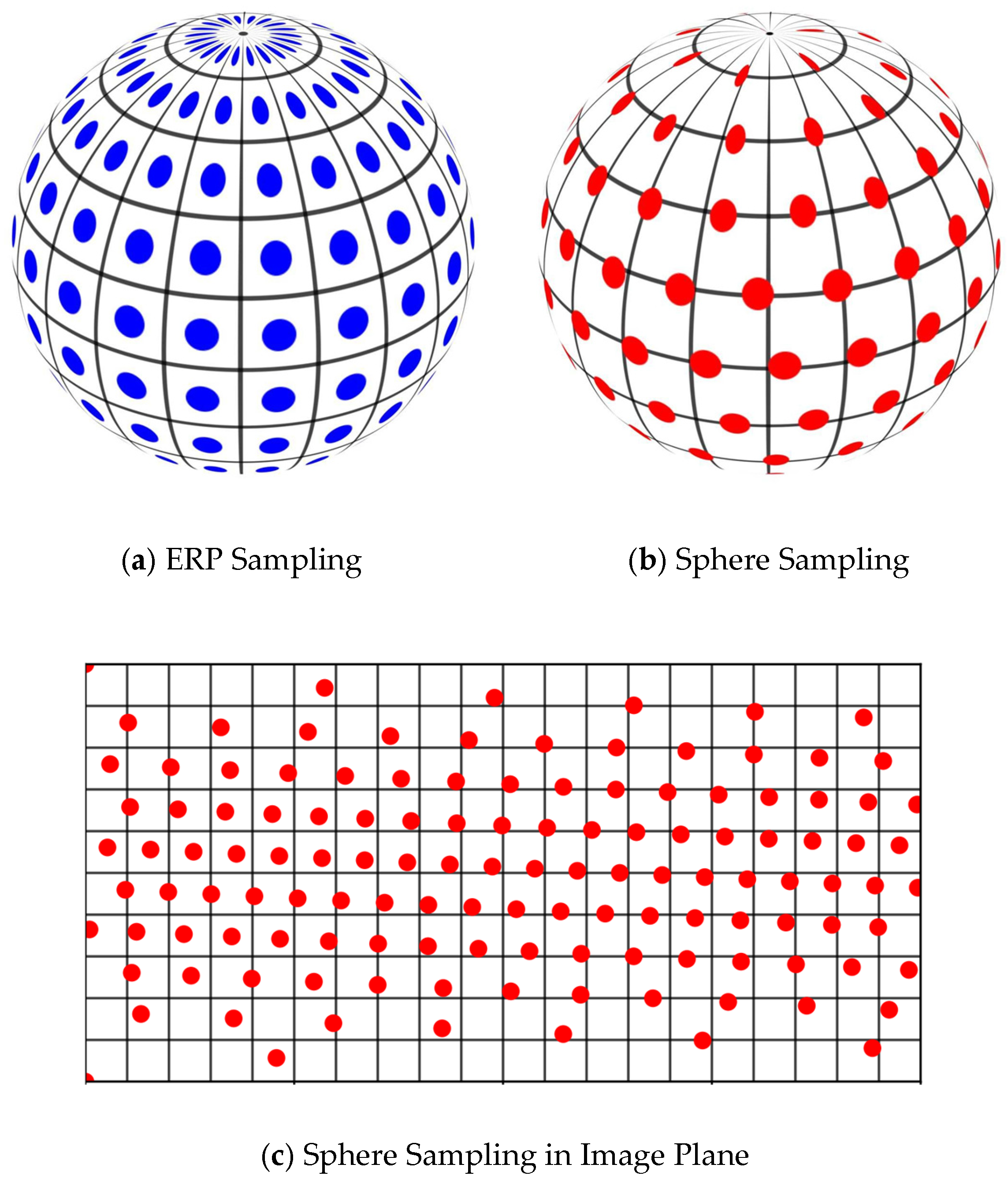
To comprehensively capture scene features and develop a global understanding of omnidirectional images, we utilize Sphere-CNN [13] to learn spherical feature representations. Traditional CNN operations, such as convolution and pooling, are designed for regular 2D images and struggle with the geometric distortions present in equirectangular images. Sphere-CNN overcomes this limitation by adapting these operations to the spherical surface, enabling more accurate feature extraction that aligns with the characteristics of SOIs. The sampling in Sphere-CNN is illustrated in Figure 2. As shown in Figure 2, compared with standard 2D convolution on ERP images, spherical convolution preserves the spatial continuity and geometric consistency of omnidirectional content. This sampling scheme enables the network to more accurately model structural distortions distributed across the sphere, which is crucial for SOI quality assessment.

In this work, let S represent the unit sphere, and its surface can be expressed as S². Each point on the sphere, denoted as $s=(\varphi ,\theta )\in S^2$, is uniquely determined by its latitude $\varphi \in [-\pi /2,\pi /2]$ and longitude $\theta \in [-\pi ,\pi ]$. Next, let $\prod$ represent the tangent plane at the point $s_{\prod }=({\varphi }_{\prod },{\theta }_{\prod })$. Points on this plane $\prod$ are represented using coordinates $x\in {ℝ}^2$. The 3 × 3 kernel sampling locations are denoted as $s(j,k)$, where $j,k\in \{-1,0,1\}$. The shape of these kernels corresponds to the step sizes ${\Delta }_{\theta }$ and ${\Delta }_{\varphi }$ of the equirectangular image at the equator. Then, the location of the filters on $\prod$ can be determined by projection as

$$x(\varphi ,\theta )={\displaystyle \frac{\cos \varphi \sin \left(\theta -{\theta }_{{\mathrm{\Pi }}_0}\right)}{\sin {\varphi }_{{\mathrm{\Pi }}_0}\sin \varphi +\cos {\varphi }_{{\mathrm{\Pi }}_0}\cos \varphi \cos \left(\theta -{\theta }_{{\mathrm{\Pi }}_0}\right)}},$$

(1)

$$y(\varphi ,\theta )={\displaystyle \frac{\cos {\varphi }_{{\mathrm{\Pi }}_0}\sin \varphi -\sin {\varphi }_{{\mathrm{\Pi }}_0}\cos \varphi \cos \left(\theta -{\theta }_{{\mathrm{\Pi }}_0}\right)}{\sin {\varphi }_{{\mathrm{\Pi }}_0}\sin \varphi +\cos {\varphi }_{{\mathrm{\Pi }}_0}\cos \varphi \cos \left(\theta -{\theta }_{{\mathrm{\Pi }}_0}\right)}},$$

(2)

Meanwhile, when applying convolution kernels at different locations on the sphere, the inverse projection needs to be used to determine the location of these kernels on the tangent plane. The inverse projection maps points on the sphere to the tangent plane centered at $s_{\prod }=({\varphi }_{\prod },{\theta }_{\prod })$ The specific inverse projection can be expressed as

$$\varphi (x,y)={\sin }^{-1}(\cos z\sin {\varphi }_{\prod }+{\displaystyle \frac{y\sin z\cos {\varphi }_{\prod }}{\rho }}),$$

(3)

$$\theta (x,y)={\theta }_{\prod }+{\tan }^{-1}({\displaystyle \frac{x\sin z}{\rho \cos {\varphi }_{\prod }\cos z-y\sin {\varphi }_{\prod }\sin z}}),$$

(4)

where $\rho =\sqrt{x^2+y^2}$, $z={\tan }^{-1}\rho$.

By establishing the projection framework and inverse projection of convolution kernels on the sphere, the global feature extraction can be implemented. To be specific, the sphere quality feature extraction branch consists of four-stage sphere convolution blocks for feature encoding. Each sphere convolution block begins with a 3 × 3 spherical convolution layer for feature extraction, followed by batch normalization and ReLU activation. A maxpooling layer is then applied to aggregate the features, and a residual connection is introduced to preserve the original feature information. After four stages of feature extraction and aggregation, the encoded features are passed to the feature interaction module. The overall network structure is illustrated in Figure 1.

3.3. Local Detail Feature Extraction

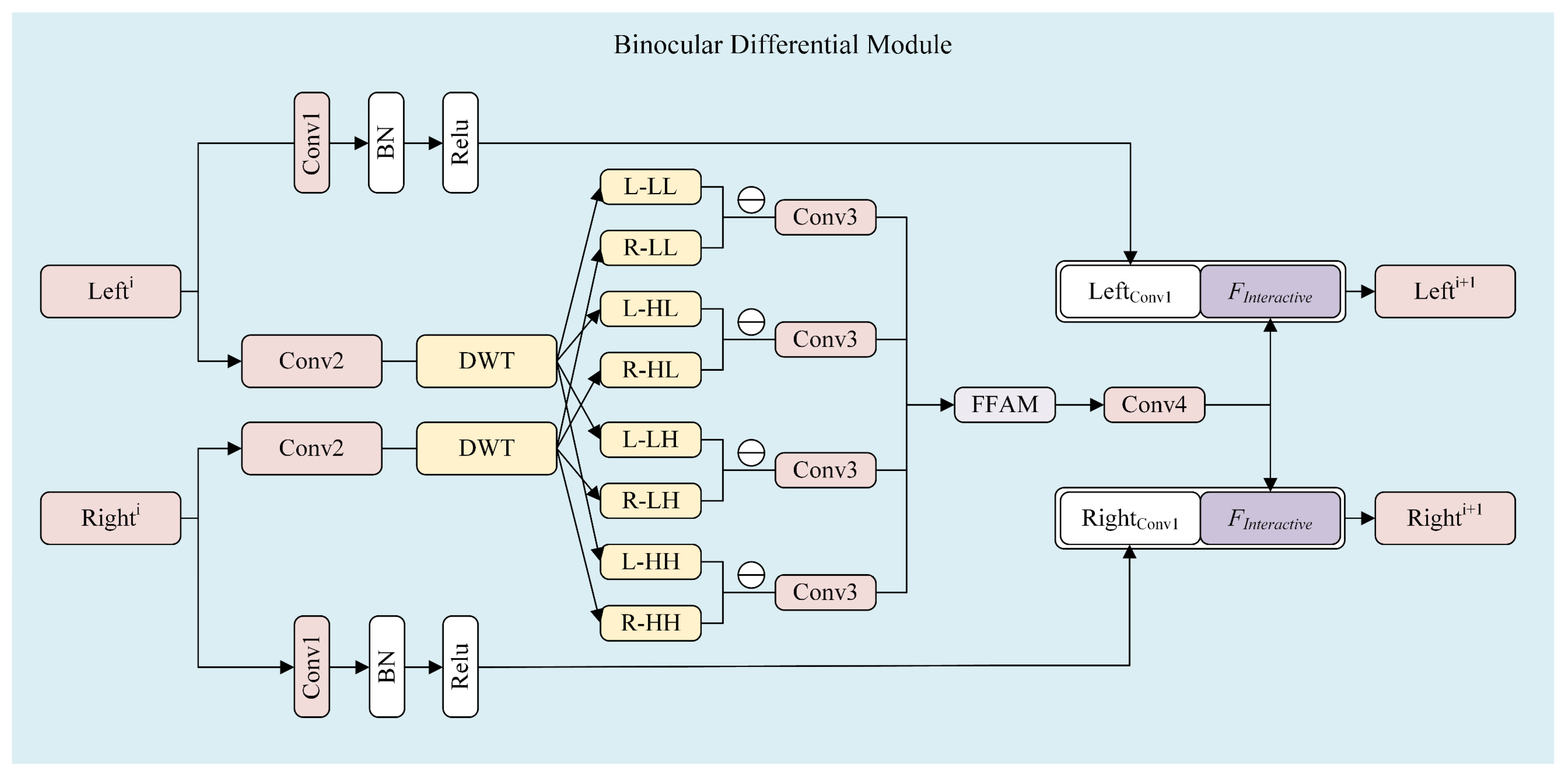
In SOIQA, binocular interaction is a crucial factor that has attracted significant research attention. Several Full-Reference (FR) SIQA methods have incorporated this aspect to simulate the human brain’s visual mechanisms [36,37]. However, the fusion strategies employed in these studies primarily rely on averaging or manually assigned weights to combine binocular visual content. Such approaches are not only time-consuming but also prone to inaccuracies, potentially compromising the effectiveness of the fusion process. To overcome these limitations, we propose a Binocular Differential Module (BDM) that leverages convolution and Discrete Wavelet Transform (DWT) to replicate the complex interactive transmission of stereoscopic visual signals in the human eye, as illustrated in Figure 3. By integrating these operations, BDM enhances the accuracy and efficiency of binocular fusion, leading to a more biologically plausible and robust quality assessment framework.

The BDM mainly consists of convolution, frequency decomposition, left–right feature differencing, and feature concatenation. Here, the inputs to the BDM are denoted as Leftⁱ and Rightⁱ, where i represents the index of the BDM, indicating the stage of feature extraction. To preserve the original visual information during the transmission of visual signals across HVS, the feature inputs are first processed through the branch started with Conv1. In this branch, the inputs undergo filtering and normalization without any additional complex processing. The number of convolution kernels in Conv1 varies across the four stages of the BDM. This initial convolution step yields the outputs Left_Conv1 and Right_Conv1, which are then aggregated for further processing.

To further enhance the neural network’s ability to extract refined visual features, a secondary branch, initiated by Conv2, is introduced and applied to the input data. Specifically, to simulate the interaction between left and right visual content, we propose a novel differential cross-convolution approach. Following the application of Conv2, the extracted features are decomposed by DWT, which is integrated for its capability to perform multi-resolution analysis and localized feature extraction. This transformation decomposes the features into four distinct sub-bands: LL (low-low), HL (high-low), LH (low-high), and HH (high-high). For each sub-band, differential feature extraction is conducted to capture additional interaction information, thereby enriching the representation of binocular interactions. The differences in each sub-band can be obtained as Equation (5). Then, D_t is obtained through a set of 1 × 1 convolution kernels, referred to as Conv3. This step further refines the extracted differential features, enhancing their discriminability for subsequent processing.

$$D_t=I_l^t-I_r^t(t=1,\dots ,4),$$

(5)

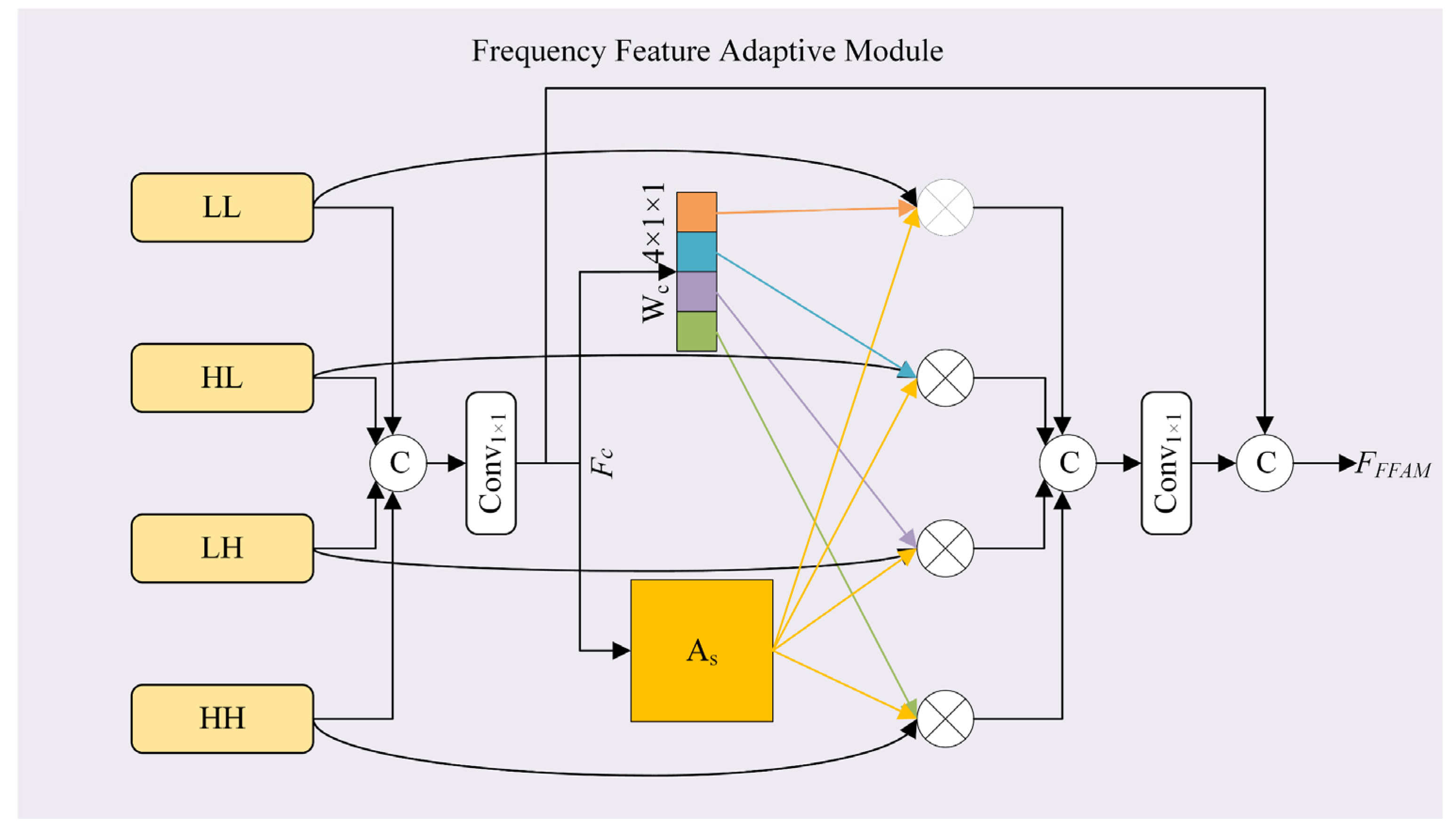
To selectively combine the four groups of features at different frequency levels, we introduce a multi-level Frequency Feature Adaptive Module (FFAM). This module assigns adaptive weights to each feature group and integrates them through a spatial attention mechanism, enabling dynamic feature fusion. By leveraging this approach, the FFAM enhances the representation of binocular interactions and generates the final interaction feature. The architecture of the proposed FFAM is illustrated in Figure 4.

Specifically, the features from the four sub-bands (LL, HL, LH, HH) are first concatenated. The concatenated features are then processed by an upsampling operation, denoted as U(⋅), followed by a 1 × 1 convolution that reduces the channel dimension from 512 to 128, obtaining the feature F_c. To effectively capture both the overall feature distribution and the salient activations within the sub-bands, we employ a combination of average pooling (Avg-Pool) and maximum pooling (Max-Pool) to learn the independent weights W_c. Avg-Pool provides a smooth representation of the feature distribution, while Max-Pool emphasizes significant activations, leveraging their complementary properties. The combined pooling results are then normalized using the sigmoid function σ(⋅), ensuring that the weights are bounded between 0 and 1. The detailed calculation of W_c can be expressed as

$$W_c=\sigma \left({\mathrm{Conv}}_{1\times 1}\left(\mathrm{Concat}\left(\mathrm{AvgPool}\left(F_c\right),\mathrm{MaxPool}\left(F_c\right)\right)\right)\right),$$

(6)

where 0 ≤ W_c ≤ 1 and ${\displaystyle \sum _{c=1}^4{W}_c}=1$.

To capture the spatial dependencies within the feature maps, a spatial attention map A_s is learned through a convolution operation on F_c, enhancing the model’s ability to focus on important spatial information. The weights W_c and the spatial attention map A_s are then multiplied with the corresponding features with different frequency components, ensuring that both spatial and channel-wise dependencies are incorporated into the final feature representation. Subsequently, the features are concatenated and processed through a 1 × 1 convolution to reduce the channel dimension from 512 to 128, retaining the most salient information while reducing computational complexity. As a result, multi-level adaptive features are generated, effectively capturing both spatial and channel-wise dependencies and improving the model’s ability to represent complex interactions within the input data.

Finally, as depicted in Figure 3, the features extracted through binocular interaction are aggregated with those from the Conv1 branch. The resulting aggregated features serve as the input for the subsequent stage of multi-stage feature extraction.

3.4. Feature Interaction and Quality Regression

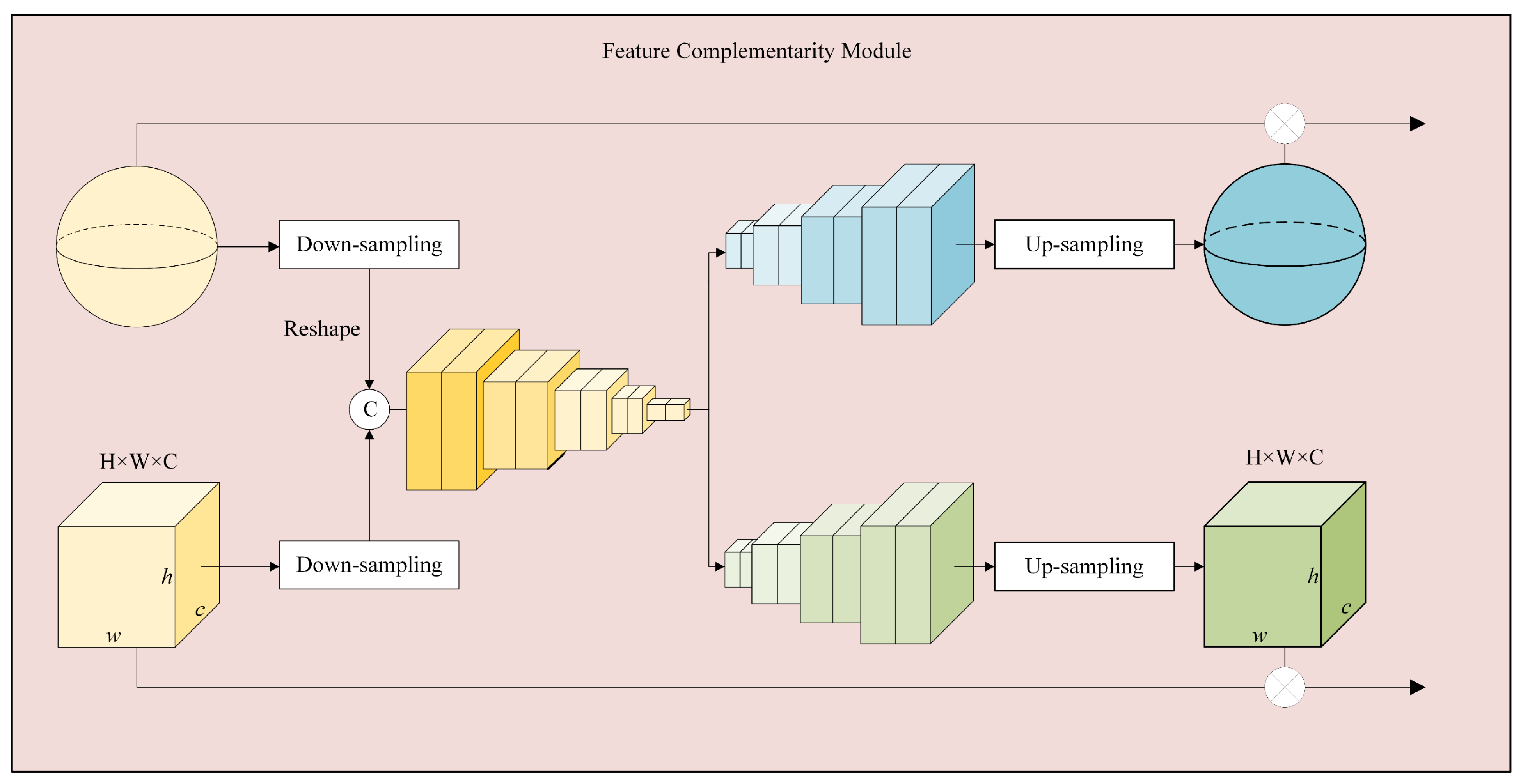
In quality assessment, integrating local and global features is crucial for capturing both fine-grained details and contextual information. To achieve this, we propose a Feature Complementarity Module (FCM) that enhances feature representation while maintaining computational efficiency. The functionality of the Feature Complementarity Module (FCM), as illustrated in Figure 5, is to effectively integrate global and local feature streams. Specifically, features from both branches are first aligned in spatial resolution using transpose convolution operations. Then, channel- and spatial-wise interactions are enabled through a gated fusion mechanism implemented with sigmoid activations. This allows the model to adaptively emphasize perceptually salient features from both the spherical and binocular perspectives. Finally, the fused representation is fed into a fully connected regression head to predict the final quality score.

Specifically, in FCM, the process begins with a series of downsampling operations, including convolution, batch normalization, Dropout, and ReLU activation. These operations progressively refine feature representations, enhancing their nonlinearity and robustness. To restore the feature map size for improved interaction and fusion with subsequent layers, a transpose convolution layer (trans-Conv) is introduced. The upsampling process further adjusts and reconstructs the features, ensuring their compatibility with local viewport processing requirements. By integrating transpose convolution, batch normalization, Dropout, and activation functions, local features are precisely processed and fused with the previously processed global features. In the later stage, an additional specialized transpose convolution layer further refines the upsampled features, ultimately generating the final output features optimized for quality assessment. This approach effectively captures and integrates both local and global features, significantly enhancing the model’s overall performance.

To further strengthen the interaction between local and global features, the FCM employs the Sigmoid activation function for feature normalization and probabilistic weighting. For local viewport features, the Sigmoid function is applied to each segmented part and multiplied with the corresponding local features, enabling targeted weighting and modulation. This mechanism allows the model to selectively highlight or suppress specific local feature information based on task requirements. Similarly, the Sigmoid-processed results are multiplied with global features to refine their representation, facilitating deep interaction and collaborative optimization between local and global features. The overall architecture of the FCM is depicted in Figure 5. By incorporating key elements of the U-Net architecture, the FCM ensures comprehensive and effective interaction between global features and local viewport features, addressing complex feature processing challenges in image quality assessment.

As described above, the viewport and global features are assigned weights using FC (which may refer to a specific operation or module, to be determined based on context), and the final prediction score is computed. For end-to-end training, the loss function is defined as

$$L={\left(Q_{\mathrm{predict} }-Q_{\mathrm{label} }\right)}^2,$$

(7)

where Q_predict represents the predicted score calculated by proposed network, and Q_label is the mean opinion score (MOS) acquired by subjective scoring.

3.5. Implementation Details

Unless otherwise specified, all convolutional layers use a kernel size of 3 × 3, stride of 1, and padding of 1. The SphereConv layers follow the formulation in [13] and are applied at two scales for multi-level spherical context aggregation. The binocular difference module (BDM) employs a discrete wavelet transform (DWT) with Haar wavelets to extract low- and high-frequency components from left–right view pairs. All activation functions are ReLU except the final regression output. Batch normalization is applied after each convolution. The feature complementarity module (FCM) uses a transpose convolution with stride 2 for feature alignment, followed by gated fusion via Sigmoid-weighted multiplication.

4. Experimental Results and Analysis

In this section, we conduct a series of experiments to evaluate the performance of the proposed method. First, we introduce the experimental protocol, including the datasets used for performance verification and the relevant evaluation metrics. Next, we assess the overall performance of the proposed method on these datasets and investigate the impact of different feature sets and parameter selections through ablation experiments. Finally, we provide an in-depth analysis and discussion of the experimental results.

4.1. Experimental Protocols

To comprehensively evaluate the performance of the proposed network, we conducted experiments on two benchmark datasets: NBU-SOID [38] and SOLID [39]. The NBU-SOID dataset consists of 12 high-quality, lossless reference stereoscopic omnidirectional images (SOIs). To generate the corresponding distorted images, the original references were processed using three different compression codecs: JPEG, JPEG2000, and HEVC. Specifically, 11 different combinations of coding parameters were used to compress the left and right views separately, including five symmetric distortion levels and six asymmetric distortion levels.

Meanwhile, the SOLID dataset comprises 312 SOIs across six original scenes with a resolution of 8192 × 4096. It includes distortions caused by BPG and JPEG compression across three depth levels. For each compression type, the zero-disparity subset contains four pairs of symmetric and four pairs of asymmetric distortions, while the intermediate-disparity and high-disparity subsets each include four pairs of asymmetric and five pairs of symmetric distortions, totaling 52 different distortion levels.

To ensure a rigorous and objective evaluation, we employed three widely used performance indicators: Pearson linear correlation coefficient (PLCC), Spearman rank correlation coefficient (SROCC), and root mean squared error (RMSE). PLCC and RMSE quantify the accuracy and consistency of predictions, while SROCC assesses the monotonicity of predicted scores. The values of PLCC and SROCC range from −1 to 1, with values closer to 1 indicating better performance. Conversely, RMSE values should be as close to 0 as possible for optimal results. Furthermore, to account for the nonlinearity in prediction scores, we applied a nonlinear regression function to map the raw objective scores, which can be expressed as

$$Q(p)={\zeta }_1·\left[{\displaystyle \frac{1}{2}}-{\displaystyle \frac{1}{1+\exp \left({\zeta }_2·\left(p-{\zeta }_3\right)\right)}}\right]+{\zeta }_4·p+{\zeta }_5,$$

(8)

where p represents the predicted score, and Q(p) is the corresponding mapped score; (ζ₁, ζ₂, ζ₃, ζ₄, ζ₅) are the parameters of the regression function.

To implement and validate the proposed network, we use PyTorch 2.4 on a dedicated server. The model is trained with the Adam optimizer (β₁ = 0.9, β₂ = 0.999); the initial learning rate is 1 × 10⁻² and is multiplied by 0.5 every 10 epochs. We adopt a batch size of 16 for 50 epochs on each dataset. A dropout rate of 0.5 is applied before the final regression layer, and the loss is the mean-squared error between the predicted and subjective MOS. The dataset is split into 80% for training and 20% for testing, ensuring every scene appears in the test set at least once. Five-fold cross-validation is performed, and original/distorted pairs from the same source are always kept within the same fold. A quick ablation on the NBU-SOID set shows that deviating the dropout rate by more than ±0.2 from the chosen 0.5 or setting the initial learning rate outside the 5 × 10⁻³–2 × 10⁻² window consistently lowers PLCC by 2–4%, confirming the adopted values.

4.2. Overall Performance Comparison

In this section, the proposed method is evaluated on two benchmark datasets and compared with various existing IQA methods. The comparative methods include: (1) seven full-reference IQA (FR-IQA) metrics, comprising three 2D FR-IQA metrics (PSNR, SSIM, GMSD) and four FR-OIQA metrics (S-PSNR [6], CPP-PSNR [7], WS-PSNR [8], WS-SSIM [14]); (2) four no-reference 2D IQA (NR-IQA) metrics (BRISQUE [40], OG [41], NIQE [42], HOSA [43]); (3) one stereoscopic IQA (SIQA) metric (SINQ [26]) and two binocular omnidirectional IQA (BOIQA) metrics (SSP-OIQA [19], VGCN [44]); and (4) two stereoscopic omnidirectional IQA (SOIQA) metrics (VP-BSOIQA [33], SOIQE [35]). It is important to note that SOIQE [35] does not have a corresponding metric in the NBU-SOID dataset. Additionally, for both the proposed method and the SINQ metric, the final SOI quality score was determined by averaging the predicted quality scores of the left and right images. To ensure the reliability of the results, only one subset was tested per evaluation round.

The experimental results, summarized in

Table 1. Performance indicators of different methods on NBU-SOID and SOLID datasets.

Type	Method	PLCC		SROCC		RMSE
		NBU-SOID	SOLID	NBU-SOID	SOLID	NBU-SOID	SOLID
2D FR-IQA	PSNR	0.781	0.710	0.791	0.673	0.596	0.653
	SSIM	0.830	0.857	0.833	0.878	0.531	0.477
	GMSD	0.862	0.827	0.864	0.779	0.484	0.521
FR-OIQA	S-PSSNR	0.809	0.720	0.827	0.663	0.561	0.643
	CPP-PSNR	0.803	0.708	0.820	0.658	0.568	0.654
	WS-PSNR	0.795	0.702	0.811	0.657	0.579	0.660
	WS-SSIM	0.832	0.877	0.835	0.889	0.529	0.446
2D NR-IQA	BRISQUE	0.747	0.797	0.592	0.583	0.573	0.471
	OG	0.811	0.827	0.753	0.691	0.509	0.507
	NIQE	0.650	0.604	0.628	0.604	0.725	0.739
	HOSA	0.741	0.564	0.710	0.539	0.641	0.766
SIQA	SINQ	0.803	0.808	0.762	0.728	0.496	0.451
OIQA	SSP-OIQA	0.740	0.765	0.689	0.695	0.553	0.541
	VGCN	0.642	0.633	0.721	0.632	0.640	0.697
SOIQA	VP-BSOIQA	0.834	0.914	0.828	0.843	0.501	0.542
	SOIQE	/	0.879	/	0.872	/	0.372
	Proposed	0.926	0.918	0.918	0.891	0.381	0.397

, indicate that the proposed method outperformed all comparative methods on both datasets, demonstrating its superior ability to assess SOI quality. Several key observations can be drawn from these results:

(1)

Compared with traditional 2D IQA methods such as PSNR and SSIM, the four FR-OIQA metrics (S-PSNR, CPP-PSNR, WS-PSNR, and WS-SSIM) specifically designed for SOIQA exhibit noticeable performance improvements. This highlights the necessity of considering latitude–longitude sampling distortions and projection-induced geometric distortions, which significantly impact human visual perception. However, these methods overlook structural and textural image features. Notably, GMSD, which effectively distinguishes image degradation, achieves a PLCC of 0.862 on the NBU-SOID dataset and 0.827 on the SOLID dataset, further emphasizing its effectiveness in capturing image quality degradation.

(2)

For no-reference IQA methods, BRISQUE and SINQ extract statistical features of natural scenes from the spatial domain, while OG utilizes relative statistical features in the gradient domain. Among them, SINQ, which incorporates stereoscopic perception, aligns more closely with human visual perception than conventional 2D NR-IQA approaches. The results suggest that a binocular masking effect occurs when viewing SOIs. However, OG outperforms SINQ in terms of PLCC due to its superior feature extraction and distortion identification capabilities on the gradient map, further demonstrating the importance of structural information in SOIQA.

(3)

Most IQA methods perform better on the SOLID dataset than on NBU-SOID, likely because SOLID contains only one type of distortion, whereas NBU-SOID includes three distinct types. The proposed method, which leverages the complementarity of global and local features, achieves the best performance. In contrast, SSP-BOIQA and VGCN, which do not account for stereoscopic perception, exhibit poor results. The VP-BSOIQA approach, integrating a binocular perception model (BPM) and an omnidirectional perception model (OPM), also delivers competitive performance.

4.3. Impacts of the Different Branch

To explore the impact of different branches, we compared the performance of the spherical global branch, the local branch, and their combination, both with and without the FCM module. The results, as illustrated in

Table 2. Performance of different branches.

Method	NBU-SOID			SOLID
	PLCC	SROCC	RMSE	PLCC	SROCC	RMSE
Global Features	0.8542	0.8216	0.5229	0.8535	0.8201	0.5250
Local Features	0.8134	0.6985	0.5850	0.8150	0.7010	0.5870
Concat (Global + Local)	0.8971	0.8514	0.4442	0.8790	0.8527	0.4796
w/FCM	0.9255	0.9181	0.3808	0.9188	0.8903	0.3970

, show that across both datasets, global spherical features outperform local visual content, suggesting that observers rely more intuitively on global features when assessing image quality.

When global and local features are directly concatenated, the performance improves, indicating that combining both types of information provides a more comprehensive representation. However, the best results are achieved when feature interaction is facilitated through the FCM. This demonstrates that the FCM effectively enhances the representation of distortions by enabling deeper interaction between global and local features.

These findings underscore the importance of integrating both global and local information for a more accurate and holistic evaluation of image quality. By leveraging feature interaction mechanisms, the model can better capture and interpret complex distortions, ultimately leading to improved quality assessment performance.

4.4. Impacts of the Binocular Differential Module

The experimental results in

Table 3. Performance of framework with different views.

Method	NBU-SOID			SOLID
	PLCC	SROCC	RMSE	PLCC	SROCC	RMSE
Left	0.8512	0.8223	0.4534	0.8823	0.8534	0.4012
Right	0.8421	0.8115	0.4612	0.8731	0.8425	0.4123
Concat (L + R)	0.8734	0.8542	0.4211	0.8912	0.8721	0.3823
BDM	0.9255	0.9181	0.3808	0.9188	0.8903	0.3970

illustrate the impact of the BDM. As can be observed, the individual performances of the left and right views are comparable, with the left view slightly outperforming the right due to asymmetric distortions in the datasets. While directly concatenating the left and right view features (Concat (L + R)) provides some improvement, it fails to fully capture the intricate interactions between binocular features. In contrast, the BDM significantly outperforms both individual branches and simple concatenation, demonstrating its ability to model binocular interactions more effectively. By leveraging differential information, the BDM enhances feature fusion, resulting in higher PLCC and SROCC values and lower RMSE across both datasets. This confirms its effectiveness in handling binocular occlusion and fusion, which are critical when observers perceive SOIs.

These findings emphasize the crucial role of the binocular differential module in improving overall system performance. By capturing subtle binocular interactions, the BDM enables a more accurate and perceptually aligned quality assessment, reinforcing its significance in stereoscopic image analysis.

4.5. Impacts of the Frequency Feature-Adaptive Module

To assess the impact of the proposed FFAM, an ablation study was conducted on the interaction features of the left and right views. The results, presented in

Table 4. Performance of different frequency feature-adaptive modules.

Method	NBU-SOID			SOLID
	PLCC	SROCC	RMSE	PLCC	SROCC	RMSE
w/o DWT	0.8325	0.8201	0.4432	0.8287	0.8165	0.4481
w/o FFAM	0.8415	0.8283	0.4376	0.8356	0.8234	0.4443
w/o DWT and FFAM	0.9255	0.9181	0.3808	0.9188	0.8903	0.3970

, highlight the module’s contribution to performance enhancement. When the input data are processed without frequency decomposition and only channel-wise adaptive adjustments are applied, a noticeable decline in evaluation performance is observed. This suggests that frequency decomposition plays a critical role in improving system effectiveness. Furthermore, it is essential to adaptively adjust features across different sub-bands after decomposition to maximize the module’s benefits. The best results are achieved when both frequency domain decomposition and adaptive feature adjustments for the left and right views are incorporated. This demonstrates that the FFAM significantly enhances overall performance by enabling more effective feature representation and interaction in the frequency domain.

4.6. Performance Comparison with Different Convolution Kernels of Global Branch

The experimental results in

Table 5. Performance of different convolution kernels.

Method	NBU-SOID			SOLID
	PLCC	SROCC	RMSE	PLCC	SROCC	RMSE
2D-Conv	0.8334	0.7564	0.4551	0.8144	0.7203	0.5670
Sphere-Conv	0.9255	0.9181	0.3808	0.9188	0.8903	0.3970

highlight the superiority of spherical convolution (Sphere-Convs) over 2D convolution (2D-Convs) in the global branch for spherical feature representation in SOIQA. Under identical hyperparameters, Sphere-Convs consistently outperform 2D-Convs across both the NBU-SOID and SOLID databases, as reflected in higher PLCC and SROCC values and lower RMSE. These improvements indicate more accurate quality prediction and enhanced feature representation. The findings align with theoretical expectations, reinforcing that spherical convolution is inherently better suited for processing spherical signals, such as those in SOIQA. This is further supported by prior research [39], which emphasizes the advantages of Sphere-Convs in capturing global structural information on spherical surfaces.

Overall, the results validate the effectiveness of using Sphere-Convs in SOIQA, demonstrating their capability to enhance feature extraction and improve perceptual quality assessment in spherical imagery.

4.7. Performance Comparison for Individual Distortion Type

To further evaluate the adaptability and robustness of the proposed method, additional performance measurements were conducted on individual distortion types. These included JPEG, JPEG2000, and HEVC distortions in the NBU-SOID database, as well as symmetric and asymmetric distortions in both datasets. For each distortion type, images were selected from the test subset, and a model trained on the entire training set, which contained all distortion types, was used to compute the quality scores. The performance comparison results are presented in

Table 6. Performance comparison with existing method for individual distortion in PLCC.

Types	Metrics	NBU-SOID					SOLID
		JPEG	JPEG2000	HEVC	Sym	Asym	Sym	Asym
2D FR-IQA	PSNR	0.732	0.851	0.798	0.854	0.673	0.804	0.503
	SSIM	0.885	0.887	0.860	0.893	0.773	0.965	0.751
	GMSD	0.960	0.926	0.897	0.921	0.794	0.883	0.710
FR-OIQA	S-PSSNR	0.771	0.875	0.838	0.879	0.718	0.812	0.591
	CPP-PSNR	0.808	0.871	0.828	0.898	0.713	0.804	0.554
	WS-PSNR	0.739	0.869	0.819	0.865	0.688	0.799	0.576
	WS-SSIM	0.894	0.885	0.854	0.894	0.775	0.973	0.785
2D NR-IQA	BRISQUE	0.919	0.877	0.683	0.837	0.613	0.875	0.745
	OG	0.925	0.896	0.858	0.818	0.815	0.871	0.718
	NIQE	0.778	0.807	0.579	0.741	0.550	0.801	0.669
	HOSA	0.790	0.849	0.602	0.811	0.663	0.658	0.413
SIQA	SINQ	0.964	0.876	0.863	0.839	0.796	0.870	0.805
OIQA	SSP-OIQA	0.927	0.887	0.865	0.831	0.747	0.839	0.761
SOIQA	VP-BSOIQA	0.973	0.949	0.948	0.893	0.873	0.982	0.907
	Propose	0.962	0.934	0.883	0.921	0.938	0.948	0.912

and

Table 7. Performance comparison with existing method for individual distortion in SROCC.

Types	Metrics	NBU-SOID					SOLID
		JPEG	JPEG2000	HEVC	Sym	Asym	Sym	Asym
2D FR-IQA	PSNR	0.744	0.853	0.785	0.870	0.690	0.843	0.423
	SSIM	0.879	0.888	0.844	0.865	0.778	0.927	0.756
	GMSD	0.939	0.925	0.888	0.895	0.794	0.889	0.588
FR-OIQA	S-PSSNR	0.788	0.882	0.831	0.898	0.729	0.829	0.416
	CPP-PSNR	0.816	0.877	0.825	0.893	0.723	0.829	0.407
	WS-PSNR	0.750	0.874	0.815	0.890	0.710	0.824	0.403
	WS-SSIM	0.886	0.890	0.846	0.870	0.777	0.934	0.784
2D NR-IQA	BRISQUE	0.879	0.688	0.604	0.693	0.471	0.759	0.473
	OG	0.907	0.834	0.771	0.782	0.697	0.819	0.566
	NIQE	0.743	0.793	0.510	0.698	0.525	0.657	0.536
	HOSA	0.766	0.849	0.564	0.779	0.601	0.738	0.414
SIQA	SINQ	0.949	0.793	0.777	0.791	0.723	0.794	0.682
OIQA	SSP-OIQA	0.881	0.848	0.801	0.715	0.627	0.779	0.693
SOIQA	VP-BSOIQA	0.957	0.889	0.875	0.862	0.833	0.927	0.777
	Propose	0.942	0.933	0.872	0.893	0.909	0.937	0.878

, with the best results among all IQA metrics highlighted in bold.

The proposed method demonstrates superior performance across various distortion types, particularly in challenging cases such as splicing distortion and asymmetric distortion. For example, in the NBU-SOID database, the proposed approach achieves a PLCC of 0.962 and an SROCC of 0.942 for JPEG distortion, outperforming other no-reference (NR) methods. Similarly, in the SOLID database, it attains a PLCC of 0.938 and an SROCC of 0.909 for symmetric distortion, as well as a PLCC of 0.948 and an SROCC of 0.937 for asymmetric distortion. Compared with traditional methods, our method consistently achieves higher PLCC and SROCC scores across both datasets. This improvement can be attributed to our use of spherical convolutions, which better preserve the spatial structure of SOIs, and to the explicit modeling of binocular perceptual asymmetry. Moreover, unlike traditional methods, which require pre-defined distortion labels, our approach remains effective under unknown and mixed distortion scenarios, highlighting its generalization ability.

These results highlight the strong adaptability and robustness of the proposed method, which leverages the deep network’s learning ability to generalize across different distortion types. While no single approach can achieve optimal performance for all distortions due to variations in feature distributions, the proposed method consistently outperforms other NR methods, particularly in complex scenarios, demonstrating its potential for real-world SOIQA applications.

5. Conclusions

In this paper, we proposed a dual-branch deep learning framework for blind quality assessment of stereoscopic omnidirectional images (SOIs). Based on the experimental results and design contributions, we conclude this work as follows:

●

Performance Summary:

(1)

The proposed framework integrates spherical structural features and binocular perceptual cues via dedicated branches and employs a feature complementarity module (FCM) to adaptively fuse global and local features. This design enables more robust and accurate quality prediction, aligning well with the nature of SOIs.

(2)

Extensive experiments on the NBU-SOID and SOLID datasets demonstrated that our method achieves superior performance, with PLCC/SROCC values of 0.926/0.918 and 0.918/0.891, respectively. Compared to state-of-the-art models, our approach shows improved generalization across different distortion types and viewing conditions.

●

Limitations:

(1)

The proposed framework assumes a fixed distortion distribution during training and lacks an explicit distortion-aware mechanism. It treats all types of distortions uniformly without dynamically adapting its feature extraction or fusion strategies. This may limit its generalization when applied to real-world scenarios with novel or mixed distortion types.

(2)

The proposed framework uses a fixed set of six viewports uniformly sampled from the spherical content. While this strategy ensures spatial coverage, it does not account for variations in user attention or perception.

(3)

The proposed framework is designed for static stereoscopic omnidirectional images and does not incorporate temporal modeling. As such, it may not fully capture perceptual variations or consistency across SOI video sequences.

●

Future Work:

(1)

We will explore dynamic viewpoint adaptation guided by saliency prediction or eye-tracking data to better match subjective perception patterns.

(2)

We will investigate integrating temporal cues, motion-aware representations, and recurrent or transformer-based architectures to extend our model to SOI video quality assessment.

(3)

We will attempt to explore distortion-invariant learning, domain generalization techniques, or meta-learning strategies to address distortion uncertainty and improve performance under mixed or novel distortion conditions.