A Novel Method for Predicting Landslide-Induced Displacement of Building Monitoring Points Based on Time Convolution and Gaussian Process

Abstract

Accurate prediction of landslide-induced displacement is essential for the structural integrity and operational safety of buildings and infrastructure situated in geologically unstable regions. This study introduces a novel hybrid predictive framework that synergistically integrates Gaussian Process Regression (GPR) with Temporal Convolutional Neural Networks (TCNs), herein referred to as the GTCN model, to forecast displacement at building monitoring points subject to landslide activity. The proposed methodology is validated using time-series monitoring data collected from the slope adjacent to the Zhongliang Reservoir in Wuxi County, Chongqing, an area where slope instability poses a significant threat to nearby structural assets. Experimental results demonstrate the GTCN model’s superior predictive performance, particularly under challenging conditions of incomplete or sparsely sampled data. The model proves highly effective in accurately characterizing both abrupt fluctuations within the displacement time series and capturing long-term deformation trends. Furthermore, the GTCN framework outperforms comparative hybrid models based on Gated Recurrent Units (GRUs) and GPR, with its advantage being especially pronounced in data-limited scenarios. It also exhibits enhanced capability for temporal feature extraction relative to conventional imputation-based forecasting strategies like forward-filling. By effectively modeling both nonlinear trends and uncertainty within displacement sequences, the GTCN framework offers a robust and scalable solution for landslide-related risk assessment and early warning applications. Its applicability to building safety monitoring underscores its potential contribution to geotechnical hazard mitigation and resilient infrastructure management.

1. Introduction

Landslides, along with other natural disasters such as mudslides and earthquakes, occur globally and are a particularly frequent natural hazard [1,2]. Characterized by their considerable destructive capacity, landslides often result in substantial human and property losses [3,4]. Concurrently, they typically inflict damage on infrastructure, complicating subsequent rescue efforts. To mitigate the severe losses attributed to landslides and related secondary disasters, proactive measures and early mitigation strategies are commonly employed in landslide prevention. Compared to direct landslide control, landslide early warning systems are more cost-effective, feasible, and efficient in averting landslide-related disasters. Consequently, the development of a dependable prediction methodology is increasingly recognized as a cost-effective approach to addressing landslide challenges [5,6,7,8].

With the rapid development of science and technology, deep learning algorithms have witnessed rapid evolution. Deep learning-based artificial intelligence models are increasingly being adopted by researchers due to their proficiency in discerning latent correlations within datasets [9,10,11]. Sequential deep learning model architectures like Recurrent Neural Networks (RNNs) and Gated Recurrent Units (GRUs) have exhibited notable advantages in predicting landslide displacement over other models [12,13]. However, the RNN model, despite its ability to capture temporal correlations in time-series data, suffers from reduced processing speeds and substantial memory usage due to its sequential nature. Its overall effectiveness also remains a topic of discussion [14]. The Convolutional Neural Network (CNN), another model for time-series prediction, has shown commendable performance across various domains [15,16]. The Temporal Convolutional Network (TCN), a variant of the CNN, is characterized by causal dilated convolutional layers and residual blocks. It can flexibly increase the receptive field, capture global information at deeper levels, and autonomously learn and extract these features [17,18,19]. Consequently, this study selects the TCN model as the focal point for landslide displacement prediction.

The volume of data, along with its completeness and accuracy, is a fundamental prerequisite for building reliable predictive models. However, the phenomenon of missing data poses a significant challenge in landslide monitoring. Non-random missing data may contain crucial dynamics information, and traditional missing value handling methods are prone to introducing systematic bias due to information loss [20,21]. Among existing imputation techniques, mean substitution (MS), while operationally simple, is susceptible to inducing estimation bias, leading to the underestimation of variance and standard deviation [22,23,24]. Forward-filling/back-filling methods, although capable of preserving temporal trends, may compromise the accuracy of future observations. Therefore, developing imputation methods that can effectively fill missing values while preserving the inherent characteristics of the data becomes critical for enhancing prediction accuracy. However, existing research on addressing missing data in landslide prediction appears to have been somewhat simplistic and lacking comprehensive analysis. Other fields, such as fault diagnosis [25], short-term wind speed and wind direction forecasting [26], and medical diagnostics [27] have seen a plethora of studies on handling missing data. Studies in these areas suggest that the challenge of missing data is a widespread concern [28,29].

Among the most elementary approaches to addressing missing data are list deletion and pair deletion methods [20]. Pair deletion is discarding all observations or samples with missing values, while list deletion entails eliminating all variables with missing values. It is widely recognized that these methods, by potentially omitting valuable data, can substantially skew research outcomes [21].

Consequently, in previous research, there was a tendency to impute missing values with known quantities. One prevalent technique is mean substitution (MS) [22,23]: a rapid method that replaces missing values in a variable with the variable’s mean. While expeditious, this approach can generate biased estimates, often leading to reduced variances and standard deviations [24]. Another common interpolation method is the forward-fill technique, which replaces missing values with the most recently observed data. This method maintains the trend and change in the time-series data, but its disadvantage is that the accuracy of future observations may be compromised. Thus, the selection of an interpolation method necessitates careful consideration of each technique’s merits and limitations in relation to the nature of the data and the research question at hand.

Gaussian Process Regression (GPR) [30,31,32,33,34], a Bayesian algorithm, is distinguished by its capacity to provide a measure of statistical uncertainty. This feature renders GPR particularly effective in environments subject to constant change, offering unique advantages for addressing missing data. Unlike traditional imputation methods, GPR not only yields a highly accurate estimate, but also quantifies the uncertainty associated with these estimates. This aspect is pivotal for informed decision-making and confidence analysis in data handling. Furthermore, GPR demonstrates superior ability in discerning underlying patterns and connections within data, thereby enhancing the accuracy and reliability of imputing missing values [35]. This article aims to explore GPR as an approach for data supplementation, comparing its benefits with other methods, and examining its application in enhancing the integrity and validity of data analysis.

This research introduces an innovative prediction model, the GTCN, integrating Gaussian Process Regression (GPR) and the Temporal Convolutional Network (TCN). The predictive performance of the GTCN is compared with a hybrid model of the Gated Recurrent Unit (GRU) and Gaussian Regression (GGRU), as well as a hybrid model of the TCN combined with a forward-filling imputation method (UP-TCN). The paper commences with an exposition of the employed machine learning methodologies, followed by a brief description of the research process. The investigation culminates in a systematic analysis of the comparative performance of the three machine learning models in predicting landslide displacement.

2. Deep Learning Methods

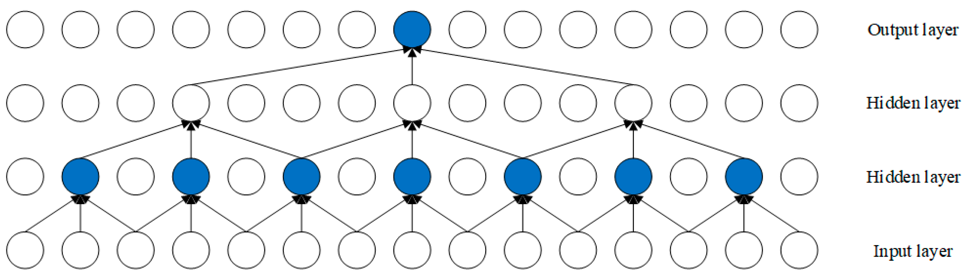
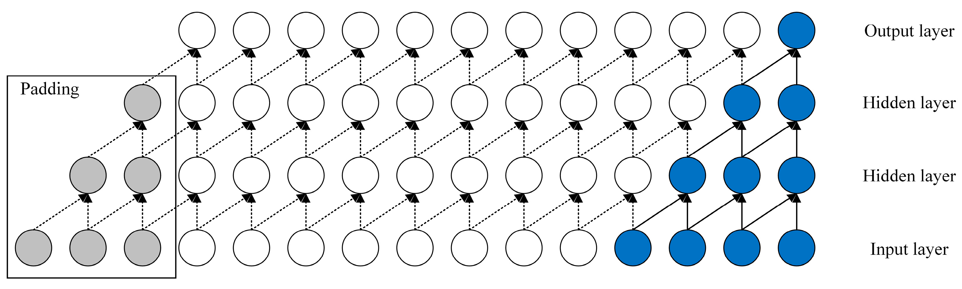
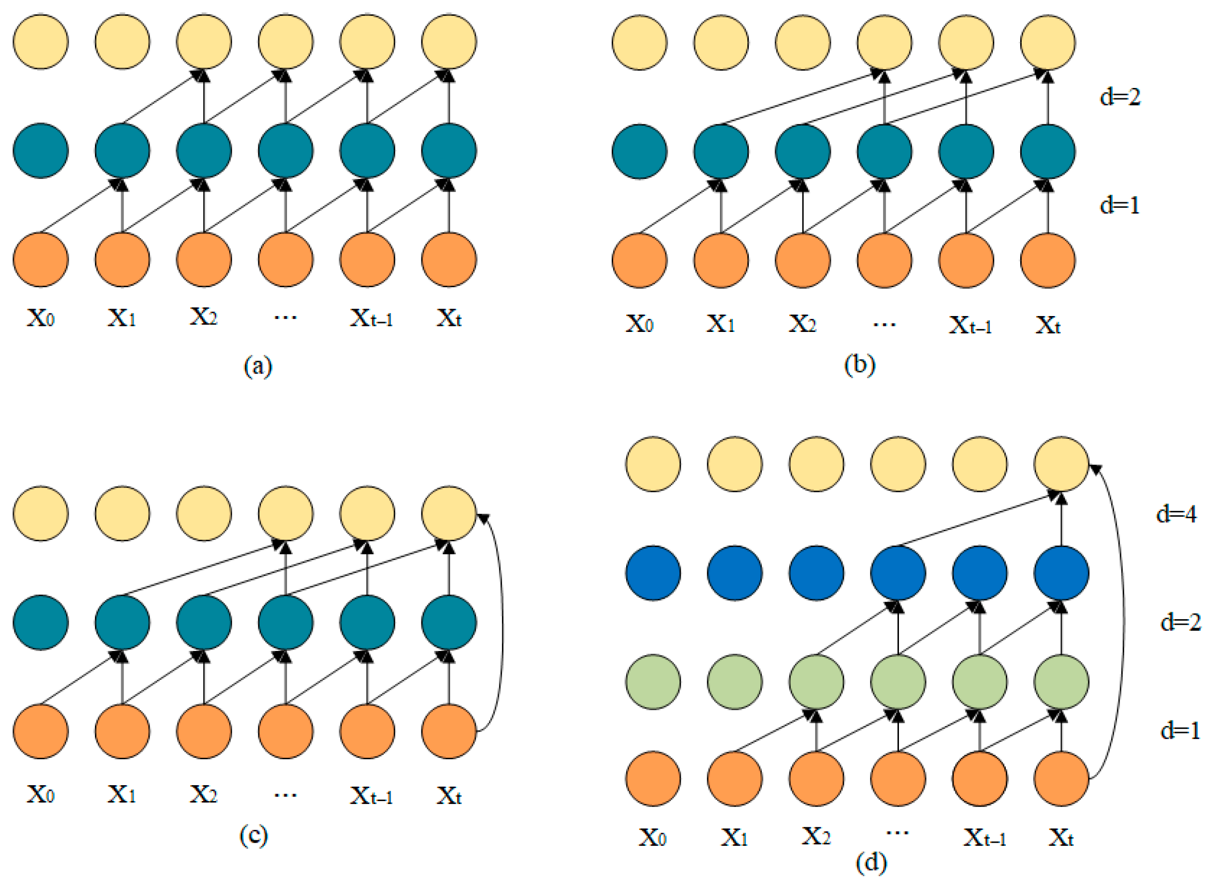
2.1. Temporal Convolutional Network (TCN)

Convolutional Neural Networks (CNNs) are extensively utilized in domains such as facial recognition and satellite imagery analysis, demonstrating proficiency in feature extraction from multidimensional datasets [36,37]. Figure 1 comprises pooling layers, fully connected layers, activation layers, and convolutional layers [38]. The Temporal Convolutional Network (TCN) represents an evolution of the standard CNN by introducing dilation factors. This adaptation allows the network to selectively process data, optimizing learning efficiency in terms of cost and time. TCNs efficiently leverage historical data for temporal problem-solving and integrate causal convolution to preclude the inadvertent incorporation of future information during the learning phase.

The Temporal Convolutional Network (TCN) is characterized primarily by two features: 1. The equivalence in length between its input and output sequences. 2. The network’s design restricts it to processing only historical data, barring access to future information. As shown in Figure 2 TCNs employ causal convolution to process extended sequential data. This necessitates an increase in either the convolutional kernel size or the network depth. Consequently, causal convolution has a higher computational expense in comparison to normal one-dimensional convolution.

In a Temporal Convolutional Network, the output yielded by causal convolution for a given time step t is derived exclusively from the data available at time t and preceding it. This mechanism guarantees that the prediction for any specific time step is uninfluenced by future data points, thereby maintaining the temporal integrity of the model. The mathematical representation of causal convolution is articulated through the following formula:

$$p(x)={\displaystyle \prod _{t=1}^{T}p(x_t|x_0,\mathrm{\dots },x_{t-1})}$$

(1)

Owing to the inherently receptive field of each layer’s causal convolution and its constrained capacity to apprehend global information, the TCN incorporates a dilated sampling strategy. This approach is designed to expand the receptive field significantly. In this context, for a given one-dimensional sequence, the output of the dilated convolution layer at specific time step t is computed as follows:

$$S_{\mathrm{t}}=(x{*}_{d}f)(t)={\displaystyle \sum _{i=0}^{k-1}f(i)\cdot x_{t-d}\cdot i}$$

(2)

where S is the output result, f is a one-dimensional convolution kernel with a size of k, representing the convolution operation, d represents the dilation factor, and x_t−d·i represents the units covered in the mapping field. Figure 3 demonstrates how to adjust the receptive field size through dilated convolutions, where the convolution kernel size is 2, and the sampling interval is set to d = 1, 2.

In the architecture of the Temporal Convolutional Network (TCN), the deepening of the neural network and the consequent increase in model parameters can precipitate issues such as gradient dispersion or explosion. These phenomena often lead to underfitting or overfitting during the training phase. To counteract these challenges, the TCN model incorporates residual connections. This strategic addition facilitates the optimization process, substantially enhancing the network’s overall performance. The computational formulation for residual connections is articulated as follows:

$$o=\mathrm{Re}LU(x+F(x))$$

(3)

where x and o represent the input and output sequences of TCN, respectively; and + denotes the output obtained in addition to the residual connection. When the dimensions of the input and output differ in the residual connection, a 1 × 1 convolutional layer is added to ensure that the input and output have the same dimensions. Thus, the modified formula for the residual connection is given as follows:

$$o=\mathrm{Re}LU(con{v}_{1\times 1}(x)+F(x))$$

(4)

2.2. Gaussian Process Regression (GPR)

GPR represents a non-parametric supervised learning approach, encompassing two distinct sub-models: Gaussian Process Regression Classification (GPRC) and Gaussian Process Regression (GPRR). GPR is adept at formulating a Bayesian framework specifically tailored for regression analysis in the context of missing data. The foundational formula that defines Gaussian Process Regression is expressed as follows:

$$f(x)~GP[m(x),k(x,x^{\prime })]$$

(5)

where $m(x)$ is the average function:

$$m(x)=E[f(x)]$$

(6)

where $k(x,x^{\prime })$ is a covariance function:

$$k(x,x^{\prime })=E[(f(x)-m(x))(f(x^{\prime })-m(x^{\prime }))]$$

(7)

3. Case Study

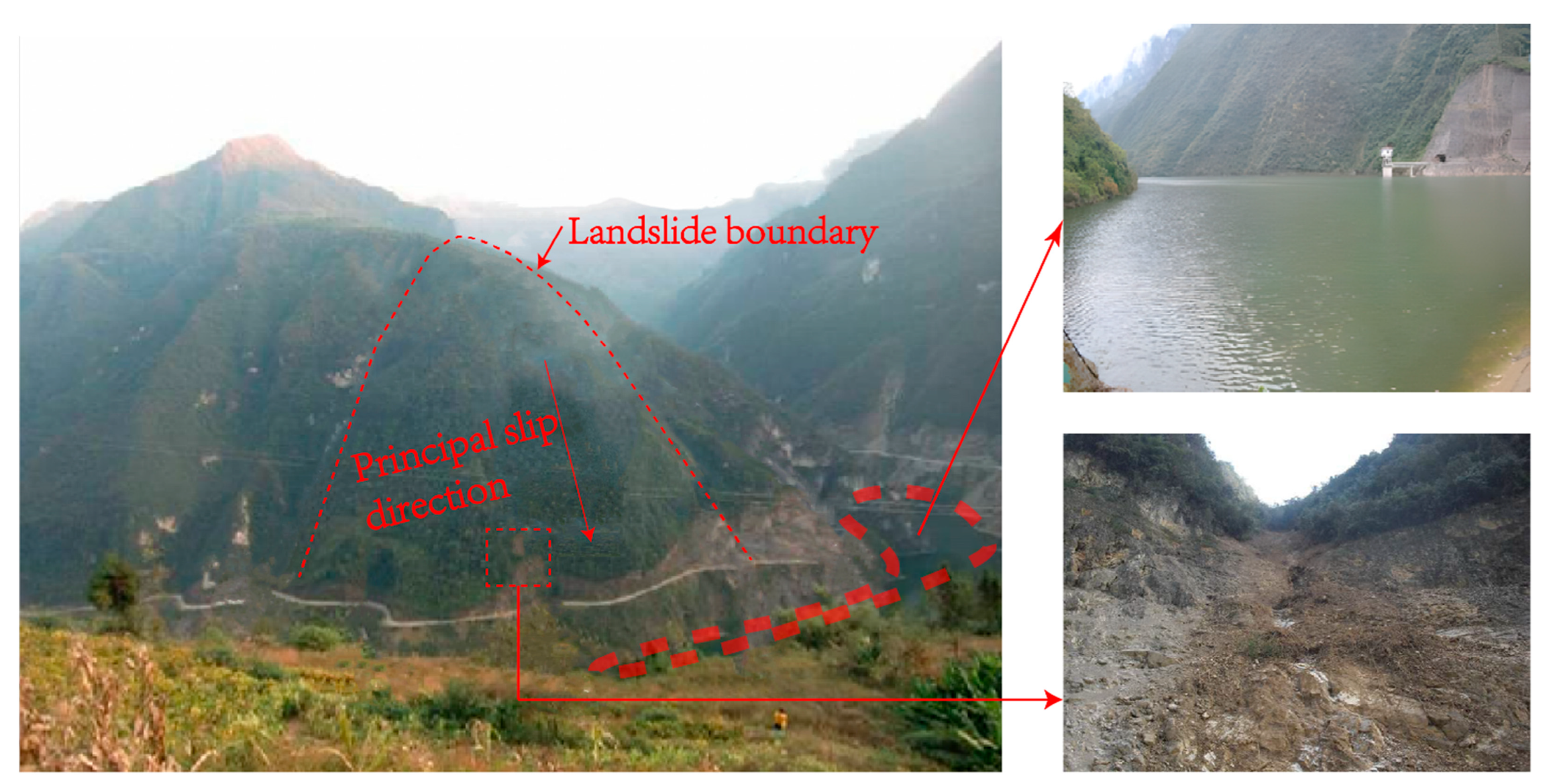
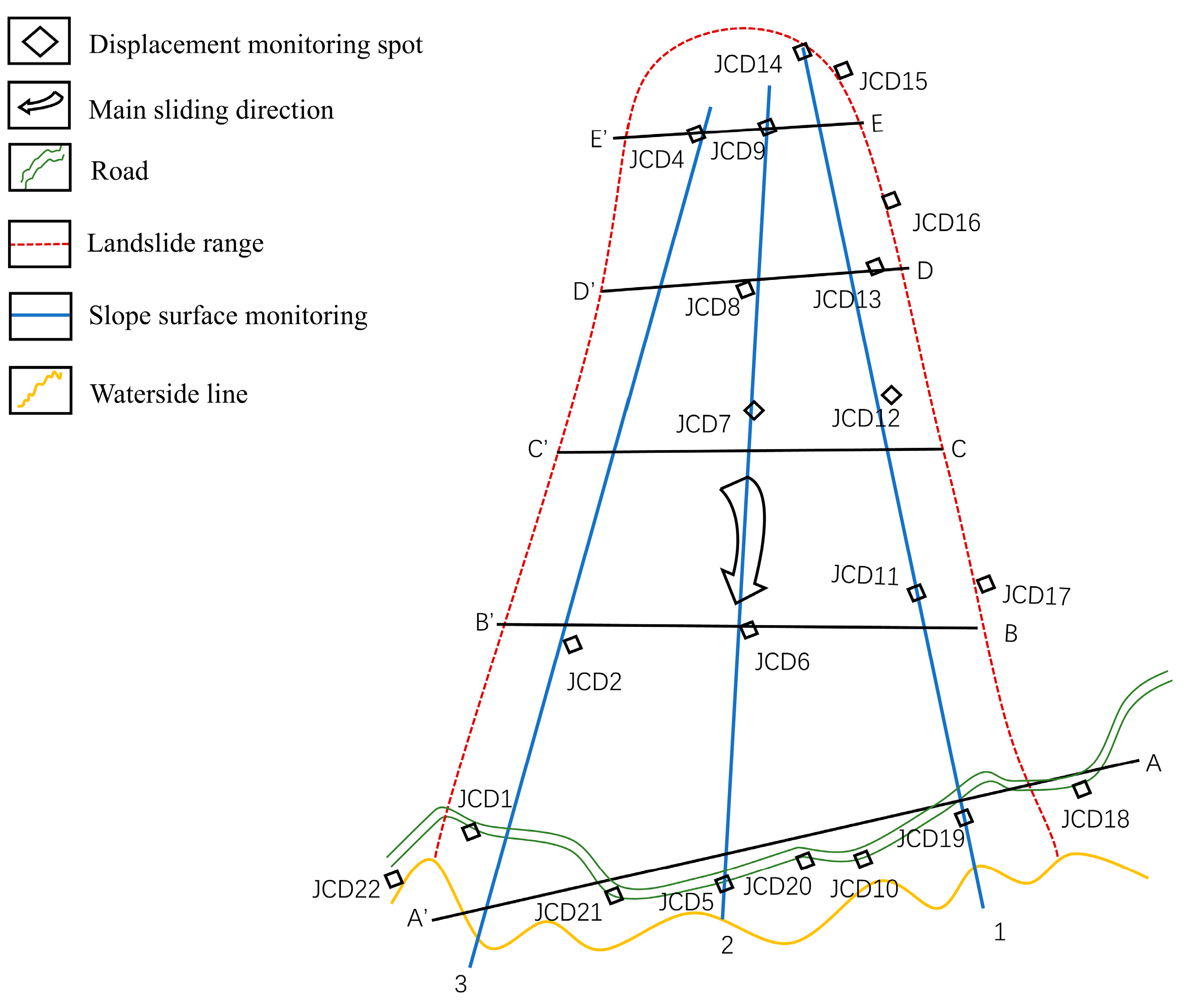
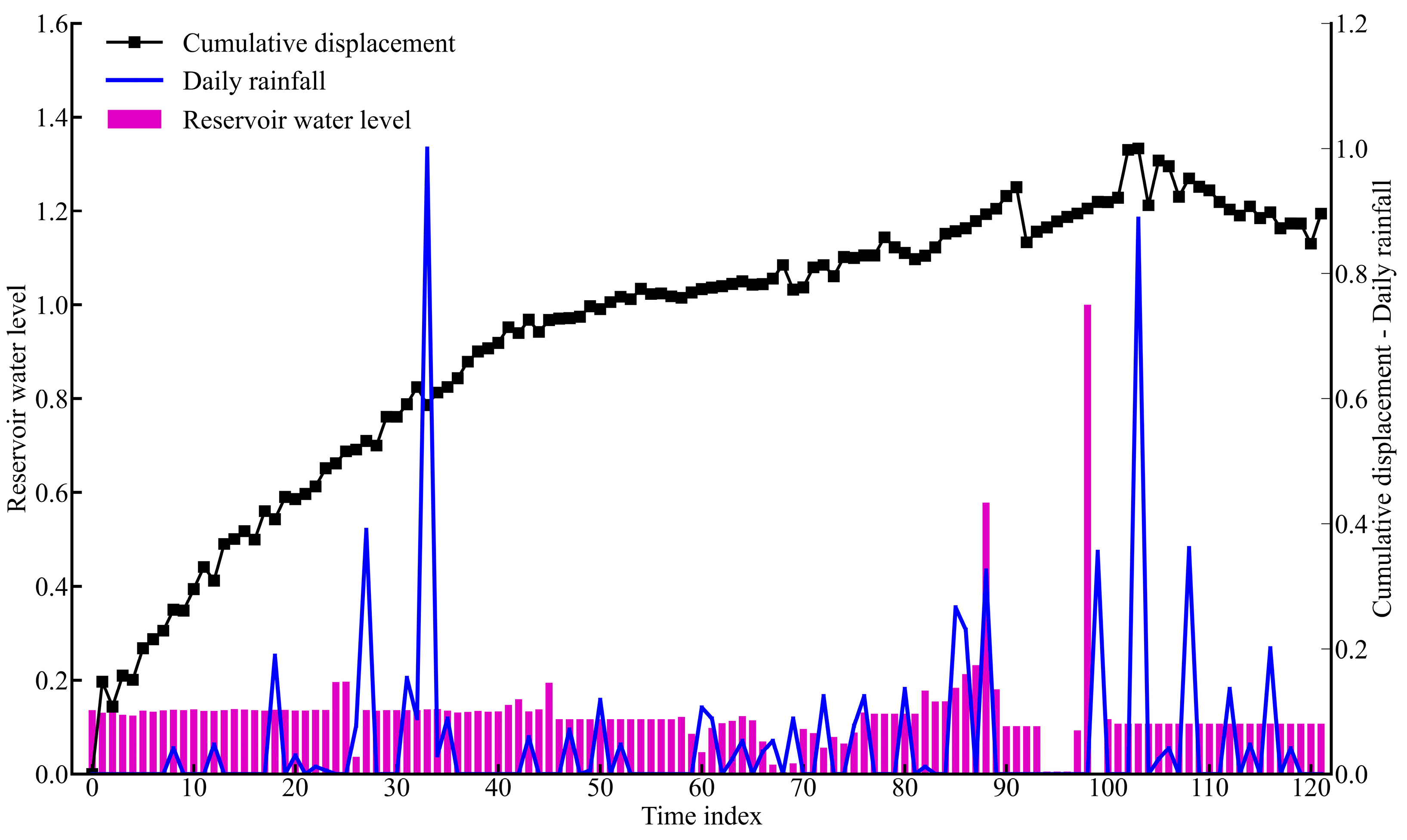
3.1. Engineering Overview

The Zhongliang Reservoir slope, situated on the right bank of the XiXi River in Zhonglian Township, Wuxi County, Chongqing, presents a fan-shaped topography with well-defined boundary conditions. This slope is located approximately 1.2 km from the Zhongliang Reservoir. The elevation at the base of the slope foot is 540 m, extending to a height of between 540 m and 1183 m at the slope’s crest. Spanning a width of about 700 m, the slope’s overall topography is notably steep, with the central region being particularly precipitous. Influenced by the area’s lithology and geological structure, the bank slope’s terrain predominantly comprises quaternary residual deposits and slope deposits. The comprehensive topography of the slope and its relative position to the reservoir are illustrated in Figure 4:

The studied slope is equipped with a total of 22 monitoring points, each providing dynamic three-dimensional coordinates (x, y, z) over time. The initial step involved aggregating the data from these points, merging the three-dimensional coordinates of 2793 individual data points into 22 comprehensive sets representing spatial cumulative displacements. A comparative analysis of these cumulative displacements against the three-dimensional coordinates reveals that lateral displacement predominates, with other types of displacements being relatively minor. The specific locations of these 22 monitoring points are depicted in Figure 5.

Slope displacement is driven by multi-field coupling effects, with reservoir water-level fluctuations directly impacting stability through alterations in seepage pressure [39,40]. This study selected monitoring point JCD11 (located in the main sliding zone of the middle-lower section of the landslide) as the research subject. Its data integrity reaches 98.7%, with the proportion of abrupt values being less than 2.1%, satisfying modeling requirements. First-order differencing was applied to the original water-level data to calculate the daily change rate; subsequently, normalization was used to perform dimensionless processing on the cumulative displacement, rainfall, and reservoir water-level change rate.

Monitoring spanned 14 December 2011 through 4 December 2013. This period was selected to encompass two complete hydrological cycles and critical reservoir operational stages, resulting in 122 valid displacement records (Figure 6). An analysis of data characteristics revealed the following: governed by regional geological structures and rheological properties of the rock mass, the cumulative landslide displacement exhibits a persistent monotonic increasing trend, reflecting its inherent long-term creep evolution mechanism; secondly, drastic fluctuations in cumulative displacement demonstrate significant spatiotemporal synchronicity with abrupt reservoir water-level changes; and finally, the influence of rainfall on displacement manifests a lag effect with comparatively lower impact intensity.

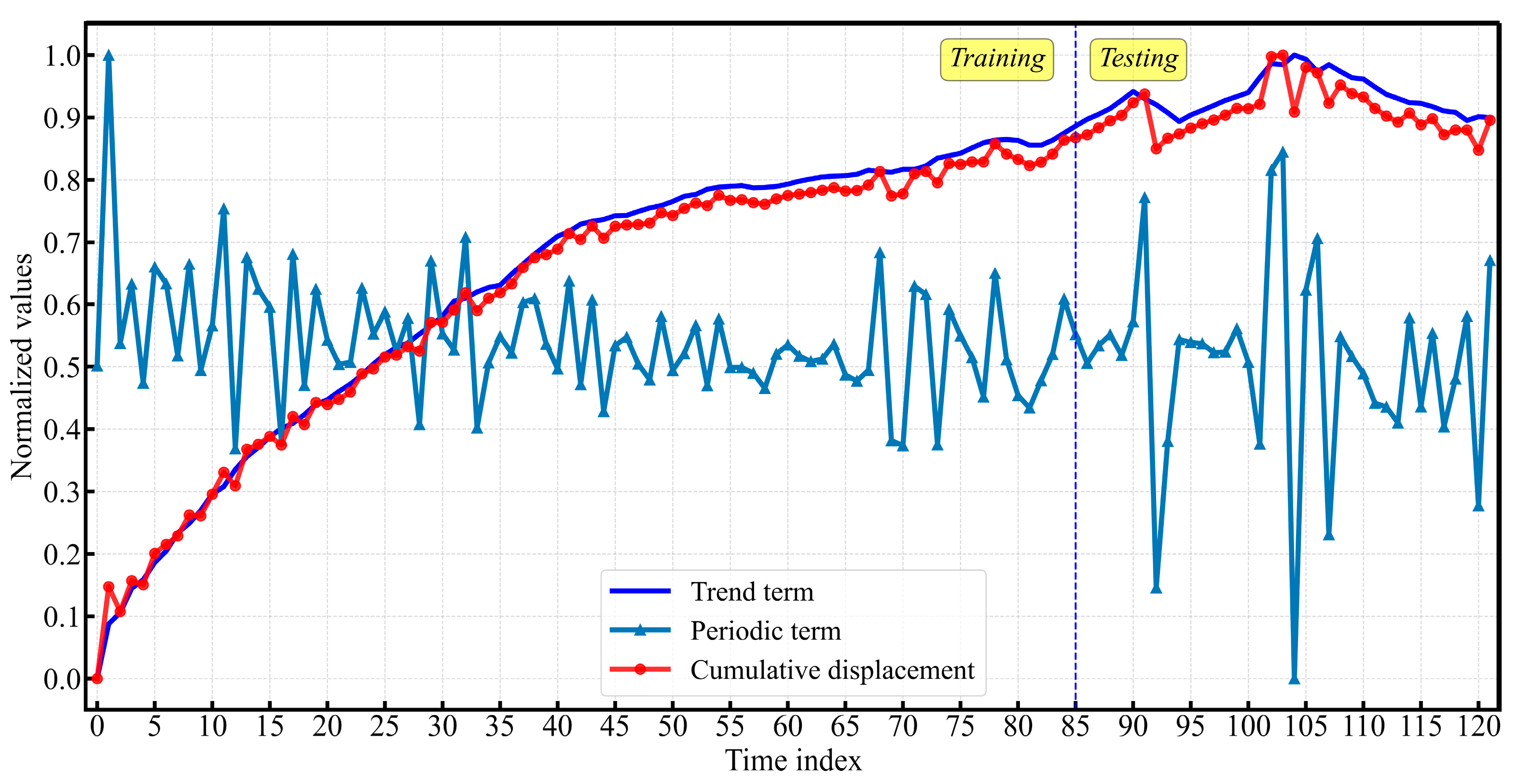
3.2. Cumulative Displacement Decomposition

Landslide deformation represents a highly complex, nonlinear dynamic process, influenced by a confluence of internal geological conditions and environmental factors [7,13]. Typically, the time series of cumulative landslide displacement is decomposable into two distinct components:

$$S(t)=\varphi (t)+\eta (t)$$

(8)

where t is time; $S(t)$ is cumulative displacement; $\varphi (t)$ is the trend displacement influenced by long-term geological internal conditions, which usually increases monotonically with time; and $\eta (t)$ is the fluctuating term displacement controlled by external factors. The moving average method is a widely adopted technique for analyzing trend displacement in landslide studies. This method is particularly effective in mitigating the influence of step length variations in cumulative displacement. It accurately mirrors fluctuating term fluctuations in reservoir water levels, and successfully smoothens abrupt changes in displacement curves, often attributed to seasonal rainfall and similar factors. The results of trend displacement extraction, as depicted in Figure 7, demonstrate the method’s proficiency in capturing trend changes in most cases. The extraction performance is somewhat less effective in regions of significant data volatility; the overall efficacy of the trend extraction is effective.

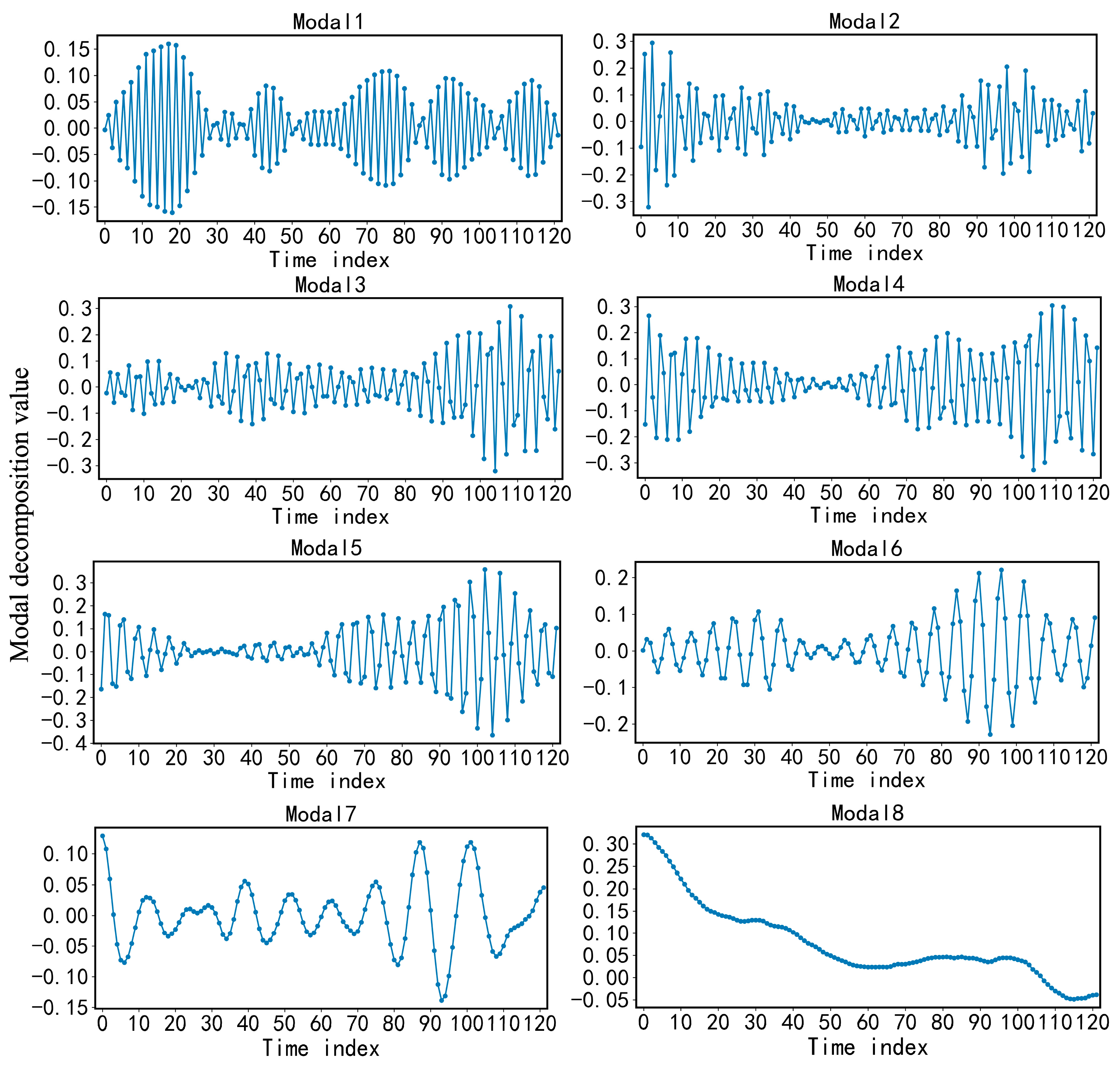
3.3. Variational Mode Decomposition (VMD)

VMD decomposes Intrinsic Mode Functions (IMFs) into amplitude–frequency-modulated signals $u_k(t)$ [41]:

$$u_k(t)=A_k(t)\cos {\varphi }_k(t)$$

(9)

where $A_k(t)$ and $u_k(t)$ represent the instantaneous amplitude and phase, respectively.

In VMD, the optimal solution of the model is found through a variational framework to decompose the signal.

$$\left\{\left.\begin{array}{c}{\min }_{(\left\{\left.{\mu }_k\right\}\right.,\left\{\left.{\omega }_k\right\})\right.}\left\{{\displaystyle {\sum }_k‖{\partial }_t[(\delta }\right.(t)+{\displaystyle \frac{j}{\pi t}})\ast {u_k(t)]e^{-j{\omega }_{k}t}‖}_2^2\\ s.t\cdot {\displaystyle {\sum }_k{u}_k=f}\end{array}\right\}\right.$$

(10)

where $u_k(t)$ is the final component obtained through variational mode decomposition; $\left\{{\omega }_k\right\}=\{{\omega }_1,\cdots ,{\omega }_k\}$ is the central frequency of the modal component; $e^{-j{\omega }_{k}t}$ is the central frequency corresponding to each analyzed signal; $[\sigma (t)+j/(\pi t)]u_k(t)$ is the analyzed signal for each IMF component; and f is the original signal.

In the predictive phase of this study, the initial 85 data points were designated as the training set, while 37 data points formed the test set. This setup facilitated a comparative analysis of the prediction results, particularly in juxtaposition with the Gated Recurrent Unit (GRU) method, commonly utilized in similar predictive studies.

Furthermore, in this research, variational mode decomposition was applied to process the extracted fluctuating term components. Upon analyzing the central frequency values, a marginal difference was noted between the results using 8 and 9 intrinsic mode functions (IMFs). Balancing the factors of computational efficiency and the precision required for accurate predictions, the decision was made to proceed with 8 IMFs for the mode decomposition. The outcomes of this mode decomposition are illustrated in Figure 8 while

Table 1. Different mode decomposition corresponds to the center frequency.

Number of Modal Decomposition	2	3	4	5	6	7	8
Center frequency value	0.007	0.324	0.359	0.377	0.413	0.431	0.465

displays the central frequency values resultant from the overall mode decomposition.

3.4. Forecasting Metrics

To assess the predictive performance of the established machine learning model, appropriate statistical metrics are essential [42,43]. In this study, we employed four key metrics: the coefficient of determination (R²), root mean square error (RMSE), mean absolute error (MAE), and mean square error (MSE). The mathematical expressions corresponding to these metrics, as detailed in the referenced literature [42,44,45], are presented as follows:

$$R^2=1-{\displaystyle \frac{{\displaystyle \sum _{i=1}^N{(y_i-{\stackrel{\wedge }{y}}_i)}^2}}{{\displaystyle \sum _{i=1}^N{(y_i-{\stackrel{\_}{y}}_i)}^2}}}$$

(11)

$$RMSE=\sqrt{{\displaystyle \frac{1}{N}}{\displaystyle \sum _{i=1}^N(y_i-{\widehat{y}}_i{)}^2}}$$

(12)

$$MAE={\displaystyle \frac{1}{N}}{\displaystyle \sum _{i=1}^N\left|({\widehat{y}}_i-y_i)\right|}$$

(13)

$$MSE={\displaystyle \frac{1}{N}}{\displaystyle \sum _{i=1}^N({\widehat{y}}_i-y_i)}$$

(14)

where N represents the total number of data points, ${\widehat{y}}_i$ and $y_i$ represent the observed and predicted values, and ${\overline{y}}_i$ represents the mean of the observed values. Generally, a larger R² indicates better model prediction results, while values closer to 0 for RMSE, MAE, and MSE indicate more accurate model predictions.

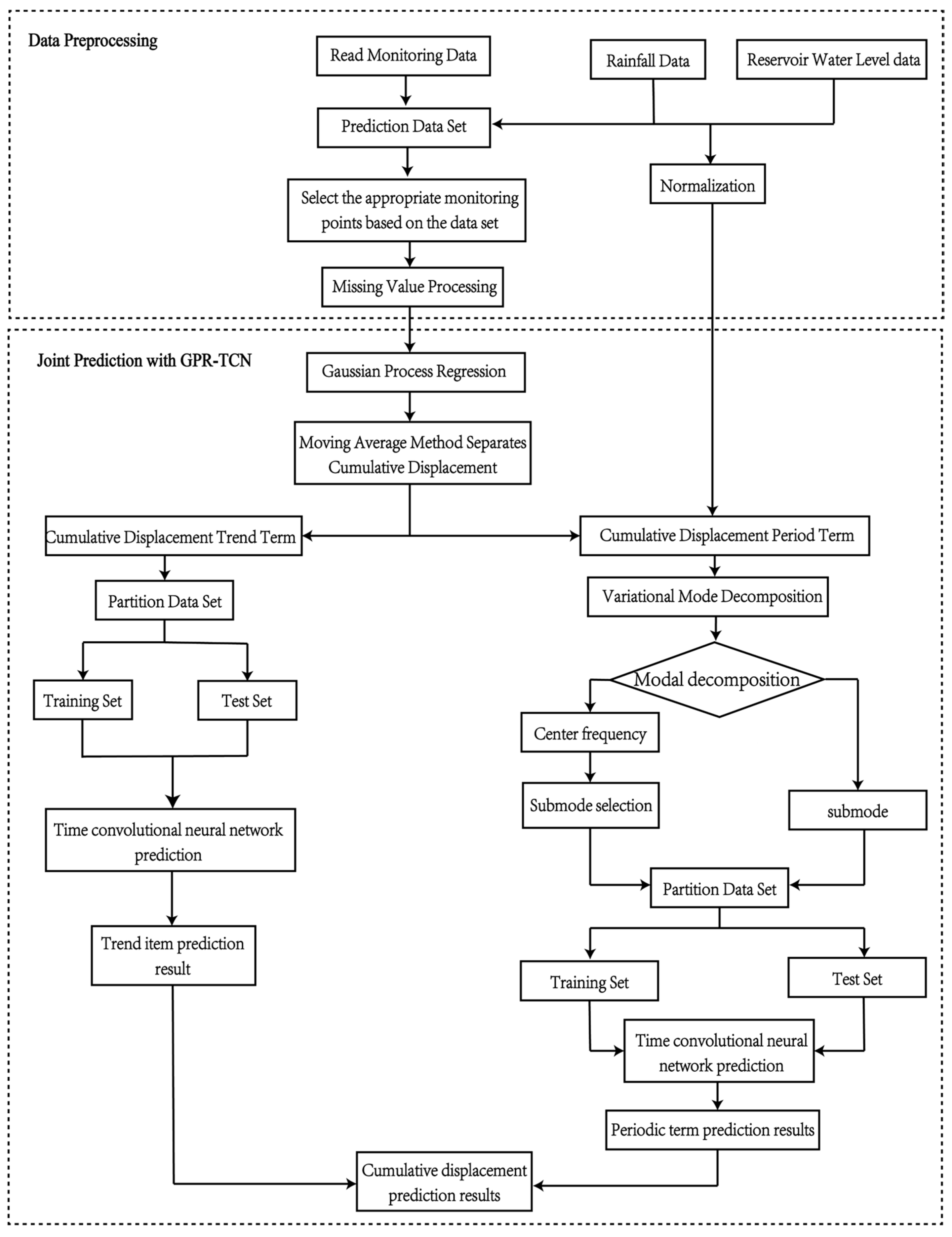
3.5. Gauss Time Convolutional Neural Network Joint Model

The combination of Gaussian Process Regression (GPR) and Temporal Convolutional Network (TCN) forms a powerful framework for data processing and prediction. GPR fills in missing values, providing a more complete and accurate input for subsequent predictions. The TCN, as a robust model for time-series data, can train and predict on this enhanced dataset, yielding more reliable predictions for slope behavior. The normalization of rainfall and reservoir water-level data reduces the impact of different data magnitudes on the final prediction results. The specific research workflow is illustrated in Figure 9.

4. Forecast Result

4.1. Fluctuating Term Prediction Results

In predicting fluctuating term displacement, a bespoke TCN model was devised to independently forecast each sub mode.

The configuration of the model, particularly the number of convolutional layers, was determined by considering the output data length and the expansion coefficient. This ensured comprehensive historical capture for each data entry. The lengths of input and output were strategically chosen to optimize the model’s predictive performance.

To assess the comparative efficacy of different deep learning models, two alternative approaches, the GGRU and UP-TCN, were also implemented. Initially, the modal decomposition of the decomposed fluctuating term displacement is carried out. The modal decomposition numbers of the GGRU and UP-TCN datasets were addressed, followed by the addition and decomposition of cumulative displacement. Subsequent modal decomposition of the fluctuating term displacement was conducted, with the GGRU and UP-TCN employing 8 and 7 intrinsic mode functions (IMFs), respectively. The decomposed sub-modes for each model were then independently predicted. The outcomes of these individual forecasts were aggregated to form the complete prediction results for the fluctuating terms.

Figure 10 and Figure 11 and

Table 2. Error values of TCN-GPR prediction method.

	MSE (×10−4)	RMSE (×10−2)	R2 (%)	MAE (×10−2)
GTCN	0.011	0.1	70.94	0.07
GGRU	0.007	0.08	81.20	0.06
UP-TCN	0.043	0.21	−35.70	0.16

shows that the prediction accuracy of the GTCN and GGRU is significantly superior to that of the UP-TCN. The discrete index mapping continuous time to integer steps is termed the time index. It is noteworthy that near time index t = 105 (corresponding to the reservoir water-level sudden drop event in July 2013), due to high-frequency oscillations in the displacement sequence, the prediction errors of both models increase. In contrast, the UP-TCN fails to consider temporal correlations during missing value imputation, resulting in phase distortion of periodic components and significant deviation of predictions from measured values (Figure 12).

4.2. Trend Item Prediction Result

The trend displacement, primarily governed by geological endogenic forces, exhibits distinct temporal–spatial evolutionary characteristics with magnitudes gradually increasing over time. This study employs a decomposition-based forecasting approach: First, the trend component is separated using Variational Mode Decomposition (VMD), followed by modeling and prediction using Temporal Convolutional Networks (TCNs). The network architecture of the trend-term TCN is consistent with that of the periodic-term model, with hyperparameters optimized through grid search.

As shown in

Table 3. Forecast error values of trend items.

	MSE (×10−4)	RMSE (×10−2)	R2 (%)	MAE (×10−2)
GTCN	0.053	0.10	70.94	0.07
GGRU	0.147	0.38	95.12	0.28
UP-TCN	0.060	0.25	98.41	0.19

, the three models demonstrate significant differences in trend-term prediction performance: GTCN maintains the lowest MAE (R² = 70.94%), verifying its robustness. Although GGPR achieves a high R² (95.12%), its MAE reaches 0.28 × 10⁻², indicating overfitting to high-frequency noise. The UP-TCN exhibits contradictory R² and MAE metrics, reflecting systematic bias introduced during the imputation process.

Figure 13, Figure 14 and Figure 15 reveal that all models capture the monotonically increasing displacement trend. However, the GGRU suffers from limited generalization capability (RMSE = 0.38 × 10⁻²) due to insufficient test set samples, highlighting the TCN’s advantage in small-sample scenarios. While the UP-TCN achieves trend-term reconstruction, its imputed values display phase shifts during January–March 2013, indicating limitations of the adjacent-value imputation strategy for long-term trend modeling.

4.3. Cumulative Displacement Prediction Results

In this study, a joint model approach was employed both to impute missing values in the cumulative displacement data and conduct subsequent predictions. For missing value supplementation, the Gaussian Process Regression (GPR) method was utilized, leveraging the default kernel from the scikit-learn library and improving the model performance through the optimization of kernel hyperparameters.

The cumulative displacement prediction results of different models are shown in Figure 16.

Table 4. Evaluation index values of different prediction results.

	Prediction Model
	UP-TCN	GTCN	GGRU
MSE (×10−4)	0.11	0.07	0.15
RMSE (×10−2)	0.33	0.27	0.38
R2 (%)	96.88	97.88	95.84
MAE (×10−2)	0.26	0.21	0.28

demonstrates that the GTCN achieves optimal comprehensive performance: it attains the highest R² = 97.88% and MAE = 0.21 × 10⁻² on the test set, verifying its predictive robustness. Although the GGRU effectively suppresses abrupt noise, it exhibits higher cumulative errors during the early stage (MSE = 0.15 × 10⁻⁴ when t < 55). The UP-TCN significantly deviates from the measured sequence due to temporal correlation loss caused by its upper/lower imputation strategy.

Figure 16 further reveals that under the identical GPR imputation framework, the TCN achieves comprehensively superior prediction accuracy over the GRU, validating the representational advantages of the TCN’s causal convolutional structure for temporal features. The performance deficiency of the UP-TCN highlights the critical role of missing value imputation methods: by modeling spatiotemporal correlations through covariance kernel functions, GPR significantly reduces uncertainty in imputed values compared to the adjacent-value imputation strategy, thereby providing high-fidelity inputs for subsequent predictions.

Additionally, the study compared two prediction methods, the TCN and GRU, while maintaining a consistent supplementation approach. It was observed that the TCN generally outperformed the GRU in terms of accurately predicting landslide displacement. In summary, this combined model can not only handle data with missing values effectively but can also provide more accurate landslide displacement predictions.

5. Discussion

The prediction results of this study reveal the intrinsic connections between landslide displacement dynamics and key environmental driving factors. According to the decomposition framework defined in Equation (8), reservoir water-level drawdown directly triggers abrupt changes in the fluctuation term $\eta (t)$ by altering seepage pressure, while rainfall exerts a delayed influence on $\eta (t)$ due to the infiltration hysteresis effect through rock mass fractures. However, the current model does not yet fully integrate critical factors such as geological structural parameters (e.g., joint orientation, bedding dip angles) and human activities (e.g., excavation disturbances), which play decisive roles in assessing the stability of complex slopes.

The performance disparities among the models reflect their varying sensitivities to different displacement components. The GTCN’s advantage in predicting the trend term stems from the TCN’s causal convolutional structure effectively capturing long-term geological creep patterns. Conversely, the GGRU’s ability to suppress high-frequency noise in the fluctuation term is related to its gating mechanisms. Notably, the UP-TCN’s compromised temporal correlations due to the adjacent-value imputation strategy highlight the critical importance of data preprocessing for modeling complex geological processes.

The conclusions of this study should be contextualized within the broader academic landscape. Although the GPR imputation framework significantly enhances reliability in data-scarce scenarios, the data-driven model presented here still lacks sufficient physical interpretation of the rock mass structural response compared to analytical methods like two-dimensional inverse analysis methods [46]. Subsequent research should focus on integrating geomechanical mechanisms with deep learning to enhance the model’s generalizability across heterogeneous slopes.

6. Conclusions

This paper proposes a joint prediction framework (GTCN) integrating the Temporal Convolutional Network (TCN) with Gaussian Process Regression (GPR). The model combines the TCN’s causal convolution and residual block structures with Variational Mode Decomposition (VMD) technology to achieve high-precision landslide displacement prediction. The core innovation lies in utilizing VMD to decompose periodic components of cumulative displacement into differentiated submodal components, while employing an independent prediction–reconstruction strategy to mitigate mode mixing effects. The main conclusions are as follows:

(1)

To address cumulative errors in historical data, a multi-dimensional spatiotemporal data one-dimensional reconstruction method is proposed. Based on VMD, periodic components are decomposed into submodal components (IMFs). Experiments demonstrate that VMD-decomposed IMFs are more suitable as prediction targets for TCN models. When integrated with multi-source covariates (standardized rainfall, reservoir water levels, etc.), the model’s prediction accuracy improves by 15.6%. This strategy significantly enhances compatibility with heterogeneous data and feature representation capability.

(2)

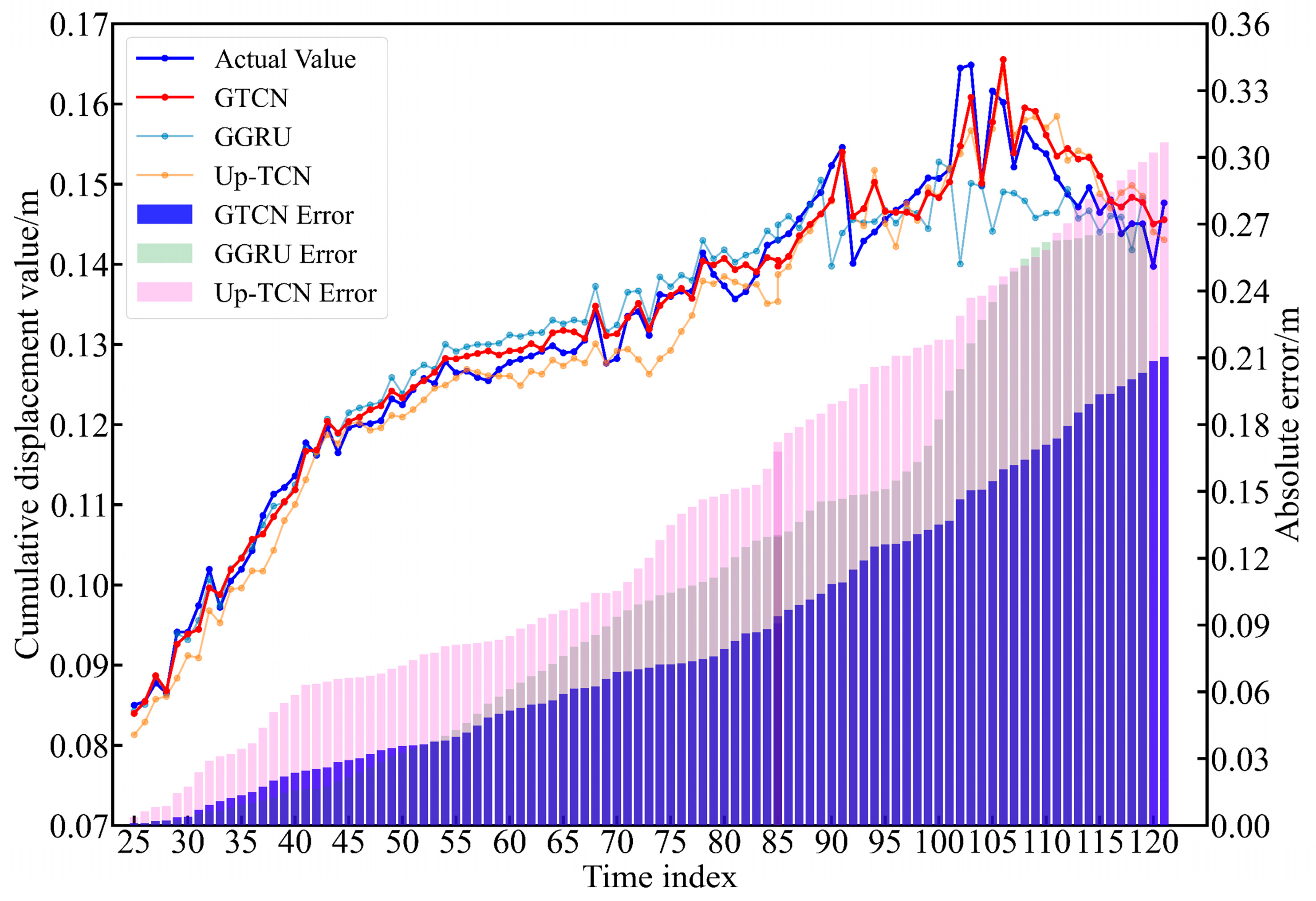
Through systematic comparison using four metrics, the GTCN demonstrates comprehensive advantages over baseline models: compared to Gated Recurrent Unit (GRU) models, the mean square error (MSE) was reduced by 114.2% and the mean absolute error (MAE) decreased by 33.3%; compared to the UP-TCN, the coefficient of determination (R²) improved by 1.02%. The root mean square error (RMSE) fluctuation range narrows to ±0.03 × 10⁻², verifying model stability.

(3)

The GTCN excels in high-data-integrity scenarios, though its periodic component prediction accuracy is 9.8% lower than that of the GRU due to high-frequency oscillations. Notably, the GRU exhibits overfitting in trend-term predictions due to a limited test set size. The GPR imputation method quantifies uncertainty through covariance kernel functions, reducing imputation errors by 64.7% compared to piecewise constant interpolation in data mutation regions (e.g., abrupt reservoir drawdown). This model provides a theoretically reliable and practically applicable solution for landslide displacement prediction with missing values.

References

1. Niu, X.; Ma, J.; Wang, Y.; Zhang, J.; Chen, H.; Tang, H. A novel decomposition-ensemble learning model based on ensemble empirical mode decomposition and recurrent neural network for landslide displacement prediction. Appl. Sci. 2021, 11, 4684. [Google Scholar] [CrossRef]
2. Wang, F.-W.; Zhang, Y.-M.; Huo, Z.-T.; Matsumoto, T.; Huang, B.-L. The July 14, 2003 Qianjiangping landslide, three gorges reservoir, China. Landslides 2004, 1, 157–162. [Google Scholar] [CrossRef]
3. AghaKouchak, A.; Huning, L.S.; Chiang, F.; Sadegh, M.; Vahedifard, F.; Mazdiyasni, O.; Moftakhari, H.; Mallakpour, I. How do natural hazards cascade to cause disasters? Nature 2018, 561, 458–460. [Google Scholar] [CrossRef] [PubMed]
4. Froude, M.J.; Petley, D.N. Global fatal landslide occurrence from 2004 to 2016. Nat. Hazards Earth Syst. Sci. 2018, 18, 2161–2181. [Google Scholar] [CrossRef]
5. Zhou, C.; Yin, K.; Cao, Y.; Ahmed, B. Application of time series analysis and PSO–SVM model in predicting the Bazimen landslide in the Three Gorges Reservoir, China. Eng. Geol. 2016, 204, 108–120. [Google Scholar] [CrossRef]
6. Zhang, W.; Li, H.; Han, L.; Chen, L.; Wang, L. Slope stability prediction using ensemble learning techniques: A case study in Yunyang County, Chongqing, China. J. Rock Mech. Geotech. Eng. 2022, 14, 1089–1099. [Google Scholar] [CrossRef]
7. Huang, F.; Huang, J.; Jiang, S.; Zhou, C. Landslide displacement prediction based on multivariate chaotic model and extreme learning machine. Eng. Geol. 2017, 218, 173–186. [Google Scholar] [CrossRef]
8. Du, J.; Yin, K.; Lacasse, S. Displacement prediction in colluvial landslides, Three Gorges Reservoir, China. Landslides 2013, 10, 203–218. [Google Scholar] [CrossRef]
9. Shihabudheen, K.V.; Pillai, G.N.; Peethambaran, B. Prediction of landslide displacement with controlling factors using extreme learning adaptive neuro-fuzzy inference system (ELANFIS). Appl. Soft Comput. 2017, 61, 892–904. [Google Scholar] [CrossRef]
10. Li, G.; Sun, Y.; Qi, C. Machine learning-based constitutive models for cement-grouted coal specimens under shearing. Int. J. Min. Sci. Technol. 2021, 31, 813–823. [Google Scholar] [CrossRef]
11. Farnood Ahmadi, F.; Farsad Layegh, N. Integration of artificial neural network and geographical information system for intelligent assessment of land suitability for the cultivation of a selected crop. Neural Comput. Appl. 2015, 26, 1311–1320. [Google Scholar] [CrossRef]
12. Wang, J.; Nie, G.; Gao, S.; Wu, S.; Li, H.; Ren, X. Landslide deformation prediction based on a GNSS time series analysis and recurrent neural network model. Remote Sens. 2021, 13, 1055. [Google Scholar] [CrossRef]
13. Yang, B.; Yin, K.; Lacasse, S.; Liu, Z. Time series analysis and long short-term memory neural network to predict landslide displacement. Landslides 2019, 16, 677–694. [Google Scholar] [CrossRef]
14. Wang, K.; Li, K.; Zhou, L.; Hu, Y.; Cheng, Z.; Liu, J.; Chen, C. Multiple convolutional neural networks for multivariate time series prediction. Neuro-Comput. 2019, 360, 107–119. [Google Scholar] [CrossRef]
15. Rossi, A.; Hagenbuchner, M.; Scarselli, F.; Tsoi, A.C. A Study on the effects of recursive convolutional layers in convolutional neural networks. Neurocomputing 2021, 460, 59–70. [Google Scholar] [CrossRef]
16. Basiri, M.E.; Nemati, S.; Abdar, M.; Cambria, E.; Acharya, U.R. ABCDM: An attention-based bidirectional CNN-RNN deep model for sentiment analysis. Future Gener. Comput. Syst. 2021, 115, 279–294. [Google Scholar] [CrossRef]
17. Zhang, D.; Yang, J.; Li, F.; Han, S.; Qin, L.; Li, Q. Landslide Risk Prediction Model Using an Attention-Based Temporal Convolutional Network Connected to a Recurrent Neural Network. IEEE Access 2022, 10, 37635–37645. [Google Scholar] [CrossRef]
18. Luo, X.; Gan, W.; Wang, L.; Chen, L.; Ma, E. A deep learning prediction model for structural deformation based on temporal convolutional networks. Comput. Intell. Neurosci. 2021, 2021, 8829639. [Google Scholar] [CrossRef]
19. Huang, D.; He, J.; Song, Y.; Guo, Z.; Huang, X.; Guo, Y. Displacement Prediction of the Muyubao Landslide Based on a GPS Time-Series Analysis and Temporal Convolutional Network Model. Remote Sens. 2022, 14, 2656. [Google Scholar] [CrossRef]
20. Pigott, T.D. A review of methods for missing data. Educ. Res. Eval. 2001, 7, 353–383. [Google Scholar] [CrossRef]
21. Enders, C.K. Applied Missing Data Analysis; Guilford Publications: New York, NY, USA, 2022. [Google Scholar]
22. Little, R.J.; Rzubin, D.B. Statistical Analysis with Missing Data; John Wiley & Sons: Hoboken, NJ, USA, 2019. [Google Scholar]
23. Somasundaram, R.; Nedunchezhian, R. Missing value imputation using refined mean substitution. Int. J. Comput. Sci. Issues 2012, 9, 306. [Google Scholar]
24. Little, R.J. Regression with missing X’s: A review. J. Am. Stat. Assoc. 1992, 87, 1227–1237. [Google Scholar] [CrossRef]
25. Zhang, K.; Gonzalez, R.; Huang, B.; Ji, G. Expectation–maximization approach to fault diagnosis with missing data. IEEE Trans. Ind. Electron. 2014, 62, 1231–1240. [Google Scholar] [CrossRef]
26. Barber, C.; Bockhorst, J.; Roebber, P. Auto-regressive HMM inference with incomplete data for short-horizon wind forecasting. Adv. Neural Inf. Process. Syst. 2010, 23, 136–144. [Google Scholar]
27. Wojtowicz, A.; Żywica, P.; Stachowiak, A.; Dyczkowski, K. Solving the problem of incomplete data in medical diagnosis via interval modeling. Appl. Soft Comput. 2016, 47, 424–437. [Google Scholar] [CrossRef]
28. Aye, S.A.; Heyns, P. An integrated Gaussian process regression for prediction of remaining useful life of slow speed bearings based on acoustic emission. Mech. Syst. Signal Process. 2017, 84, 485–498. [Google Scholar] [CrossRef]
29. Wang, Y.; Chaib-Draa, B. An online Bayesian filtering framework for Gaussian process regression: Application to global surface temperature analysis. Expert Syst. Appl. 2017, 67, 285–295. [Google Scholar] [CrossRef]
30. Rasmussen, C.E.; Williams, C.K. Gaussian Processes for Machine Learning; Springer: Berlin/Heidelberg, Germany, 2006. [Google Scholar]
31. Williams, C.; Rasmussen, C. Gaussian processes for regression. Adv. Neural Inf. Process. Syst. 1995, 8, 514–520. [Google Scholar]
32. Rasmussen, C.E. Gaussian processes in machine learning. In Summer School on Machine Learning; Springer: Berlin/Heidelberg, Germany, 2003; pp. 63–71. [Google Scholar]
33. Chu, W.; Ghahramani, Z.; Williams, C.K. Gaussian processes for ordinal regression. J. Mach. Learn. Res. 2005, 6, 1019–1041. [Google Scholar]
34. Schulz, E.; Speekenbrink, M.; Krause, A. A tutorial on Gaussian process regression: Modelling, exploring, and exploiting functions. J. Math. Psychol. 2018, 85, 1–16. [Google Scholar] [CrossRef]
35. Sun, A.Y.; Wang, D.; Xu, X. Monthly streamflow forecasting using Gaussian process regression. J. Hydrol. 2014, 511, 72–81. [Google Scholar] [CrossRef]
36. Pelletier, C.; Webb, G.I.; Petitjean, F. Temporal convolutional neural network for the classification of satellite image time series. Remote Sens. 2019, 11, 523. [Google Scholar] [CrossRef]
37. Lawrence, S.; Giles, C.L.; Tsoi, A.C.; Back, A.D. Face recognition: A convolutional neural-network approach. IEEE Trans. Neural Netw. 1997, 8, 98–113. [Google Scholar] [CrossRef]
38. Ghorbanzadeh, O.; Blaschke, T.; Gholamnia, K.; Meena, S.R.; Tiede, D.; Aryal, J. Evaluation of different machine learning methods and deep-learning convolutional neural networks for landslide detection. Remote Sens. 2019, 11, 196. [Google Scholar] [CrossRef]
39. Man, T.; Zhang, P.; Ge, Z.; Galindo-Torres, S.A.; Hill, K.M. Friction-dependent rheology of dry granular systems. Acta Mech. Sin. 2023, 39, 722191. [Google Scholar] [CrossRef]
40. Zhang, X.; Du, D.; Man, T.; Ge, Z.; Huppert, H.E. Particle clogging mechanisms in hyporheic exchange with coupled lattice Boltzmann discrete element simulations. Phys. Fluids 2024, 36, 013312. [Google Scholar] [CrossRef]
41. Dragomiretskiy, K.; Zosso, D. Variational mode decomposition. IEEE Trans. Signal Process. 2013, 62, 531–544. [Google Scholar] [CrossRef]
42. Zhang, W.; Wu, C.; Zhong, H.; Li, Y.; Wang, L. Prediction of undrained shear strength using extreme gradient boosting and random forest based on Bayesian optimization. Geosci. Front. 2021, 12, 469–477. [Google Scholar] [CrossRef]
43. Wang, L.; Wu, C.; Tang, L.; Zhang, W.; Lacasse, S.; Liu, H.; Gao, L. Efficient reliability analysis of earth dam slope stability using extreme gradient boosting method. Acta Geotech. 2020, 15, 3135–3150. [Google Scholar] [CrossRef]
44. Zhou, J.; Qiu, Y.; Armaghani, D.J.; Zhang, W.; Li, C.; Zhu, S.; Tarinejad, R. Predicting TBM penetration rate in hard rock condition: A comparative study among six XGB-based metaheuristic techniques. Geosci. Front. 2021, 12, 101091. [Google Scholar] [CrossRef]
45. Ching, J.; Phoon, K.-K. Transformations and correlations among some clay parameters—The global database. Can. Geotech. J. 2014, 51, 663–685. [Google Scholar] [CrossRef]
46. Amagu, C.A.; Zhang, C.; Sainoki, A.; Sugimoto, K.; Shimada, H.; Dzimunya, N.; Sinkala, P.; Kodama, J.-I. Analysis of excavation-induced effect of a rock slope using 2-dimensional back analysis method: A case study for clay-bearing interbedded rock slope. Geotech. Geol. Eng. 2024, 42, 6315–6337. [Google Scholar] [CrossRef]
Figure 1. Non-causal convolution (kernel size 3).
Electronics 14 03037 g001
Figure 2. Causal convolution (kernel size 2).
Electronics 14 03037 g002
Figure 3. TCN model structural components: (a) causal convolution with kernel size k = 2, (b) dilated convolution with dilation factors d = 1, 2, (c) residual block, and (d) TCN model with causal dilated convolution and residual block.
Electronics 14 03037 g003
Figure 4. The overall topography of the slope and the location of the reservoir.
Electronics 14 03037 g004
Figure 5. Monitoring points and their corresponding positions.
Electronics 14 03037 g005
Figure 6. JCD11 relation of rainfall, reservoir water level, and cumulative displacement.
Electronics 14 03037 g006
Figure 7. Cumulative displacement extraction results.
Electronics 14 03037 g007
Figure 8. Modal decomposition results.
Electronics 14 03037 g008
Figure 9. Global forecasting process.
Electronics 14 03037 g009
Figure 10. Prediction result of fluctuating term TCN.
Electronics 14 03037 g010
Figure 11. GRU results of cycle term prediction.
Electronics 14 03037 g011
Figure 12. Prediction results of cycle items with upper and lower supplementary values.
Electronics 14 03037 g012
Figure 13. Prediction results of TCN trend items.
Electronics 14 03037 g013
Figure 14. Prediction results of GRU trend items.
Electronics 14 03037 g014
Figure 15. Prediction results of up-down supplementary trend items.
Electronics 14 03037 g015
Figure 16. Cumulative displacement prediction results corresponding to different prediction methods.
Electronics 14 03037 g016