Consistency-Oriented SLAM Approach: Theoretical Proof and Numerical Validation

Abstract

Simultaneous Localization and Mapping (SLAM) has long been a fundamental and challenging task in robotics literature, where safety and reliability are the critical issues for successfully autonomous applications of robots. Classically, the SLAM problem is tackled via probabilistic or optimization methods (such as EKF-SLAM, Fast-SLAM, and Graph-SLAM). Despite their strong performance in real-world scenarios, these methods may exhibit inconsistency, which is caused by the inherent characteristic of model linearization or Gaussian noise assumption. In this paper, we propose an alternative monocular SLAM algorithm which theoretically relies on interval analysis (iMonoSLAM), to pursue guaranteed rather than probabilistically defined solutions. We consistently modeled and initialized the SLAM problem with a bounded-error parametric model. The state estimation process is then cast into an Interval Constraint Satisfaction Problem (ICSP) and resolved through interval constraint propagation techniques without any linearization or Gaussian noise assumption. Furthermore, we theoretically prove the obtained consistency and propose a versatile method for numerical validation. To the best of our knowledge, this is the first time such a proof has been proposed. A plethora of numerical experiments are carried to validate the consistency, and a preliminary comparison with classical EKF-SLAM in different noisy situations is also presented. Our proposed iMonoSLAM shows outstanding performance in obtaining reliable solutions, highlighting the potential application prospect in safety-critical scenarios of mobile robots.

1. Introduction

Simultaneous Localization and Mapping (SLAM) is a fundamental robotics problem involving the construction of a map of an unknown environment and the estimation of the robot’s pose within that environment based on data collected from onboard sensors. Reliable solutions to the SLAM problem are critical for the effective deployment of robots across a wide range of applications, including environment reconstruction, self-driving cars, aerial drones, autonomous mobile robots, and planetary exploration [1]. To address the complexities of SLAM, various theoretical frameworks and technological approaches have been developed. The majority of current approaches use probabilistic methods that rely on the propagation of probability distributions. Alternatively, interval analysis-based methods have been developed, which do not depend on any probabilistic assumptions. Instead, they model uncertainty by assuming that measurement noise is bounded within real intervals.

Robotic localization and mapping problems have traditionally been addressed using probabilistic approaches, with Kalman filters and particle filters [2,3] being among the most widely adopted techniques. While probabilistic methods perform reliably in many real-world applications, they may encounter inconsistencies under specific conditions [4,5]. This limitation is well acknowledged by researchers in this field [6,7]. A primary cause of this inconsistency is the underlying assumption that measurement noise can be accurately modeled using known probability density functions. Furthermore, some methods like Extended Kalman Filtering (EKF) need a linearization process in case of nonlinear models. However, robotic systems in practical applications are typically nonlinear, and many sensors either deviate from the Gaussian noise assumption or operate without clearly defined noise models [8]. Consequently, these methods can only associate a probability to an estimated result (the robot pose or landmark positions), but the real solution cannot be guaranteed to be located in the probabilistically defined region [9,10] (inconsistent issue).

To address the SLAM problem, interval analysis [11] presents a different perspective. Rather than assuming specific probability distributions for sensor noise, interval methods operate under the premise that sensor uncertainties are confined within known deterministic bounds. This approach aligns well with practical conditions, as sensor manufacturers typically provide maximum and minimum error specifications under defined operating conditions that can be directly interpreted as error bounds. Interval analysis-based methods leverage these bounded errors by recursively propagating them through consistent estimation techniques combined with systematic searching algorithms. Unlike probabilistic approaches, interval methods provide guaranteed enclosures of the true state, ensuring that no feasible solutions are excluded. The effectiveness of interval analysis was proved by the results of aforementioned studies. However, very few works are dedicated to studying, theoretically, the obtained consistency. In [12], the authors introduced a novel theoretical framework, which was used to establish consistency conditions for robotic mapping in nonlinear, non-Gaussian scenarios. However, their formulation relies on the availability of certain anchoring landmarks.

Building upon our previous work [13,14,15], the main contribution of this work is as follows:

• We propose an interval analysis-based monocular SLAM algorithm that employs an undelayed, bounded-error parametric approach, coupled with a consistency-preserving solution technique. The consistency performance was tested and compared through numerical experiments.
• We present for the first time, a theoretical study and proof of the obtained consistency of the interval analysis-based SLAM method, which could promote applications in safety-critical robotic scenarios.
• In addition, we propose a novel consistency-evaluation method for experimentally validating the consistency of the interval analysis-based location and mapping algorithm.

The structure of the paper is as follows: Section 2 provides an overview of the related works and the theory of interval analysis, while Section 3 introduces the proposed iMonoSLAM algorithm. Section 4 details the theoretical analysis and proof of the consistency property of the proposed iMonoSLAM algorithm. Section 5 presents the simulation results to verify the feasibility and consistency of iMonoSLAM. Section 6 presents the comparison results between iMonoSLAM and EKF-SLAM. Section 7 presents a discussion of the paper and proposes some prospects of future works.

2. Overview of Interval Analysis and Constraint Propagation

The theoretical foundation of this study lies in interval analysis and constraint propagation. We will firstly give a brief introduction to related works and the fundamental knowledge in this section.

Di Marco [16] introduced the first interval analysis-based SLAM algorithm. Robot localization was represented by the state variable x, y, and $\theta$, with its volume updating based on proprioceptive inputs from odometers and exteroceptive measurements from range and bearing sensors. Landmarks were modeled by parallelotopes (generalized parallelograms). The authors in [17] proposed their interval analysis-based SLAM algorithm using the Set Inversion Via Interval Analysis [18] algorithm. It integrated odometers with a stereoscopic omnidirectional vision sensor, delivering a full ${360}^{\circ }$ view of the environment. Both the robot’s location and the positions of landmarks were modeled using subpavings [18]. The landmark was estimated by computing the intersection between the existing landmark subpaving and the newly obtained one. Simulation results have shown that the estimations of the subpavings are robust and coherent. The authors [19] presented CUIK (Complete Universal Inverse Kinematics) to address the SLAM problem, updating landmark estimates through constraints that connect the robot’s localization with the landmarks. Different from [16], each landmark was modeled by a 3D position box rather than a parallelotope. Such a representation facilitates the computation using CUIK. Indoor experiments using sonar have demonstrated its effectiveness. The SLAM algorithm presented in [20] was based on constraint propagation techniques. The fundamental idea behind this method is to represent the SLAM problem as a constraint satisfaction problem, enabling the use of Interval Constraint Propagation (ICP) algorithms, which are particularly effective for solving such formulations. Experiments [21,22] were conducted on an underwater robot platform showing that the algorithm gives a consistent result. Later, another paradigm of interval-based SLAM algorithms was published in [21,23] to address the range-only SLAM problem with occupancy maps or indistinguishable landmarks. The SLAM problem was formulated as a hybrid constraint satisfaction problem, in which the variables could be real numbers, vector trajectories, or subsets of ${\mathbb{R}}^n$. Simulated test cases were designed to demonstrate its effectiveness in producing guaranteed sets that enclose both the robot’s trajectory and the map space. The author in [24] presented an interval SLAM algorithm for 3D mapping using a RGB-D sensor. Computer vision techniques were used to extract polar landmarks from the RGB images and interval methods are used to estimate landmark positions. The experimental results were evaluated against the conventional least-squares method to assess the consistency and accuracy. We previously modeled the monocular SLAM as ICSP and took advantage of the ICP algorithms to obtain consistent solutions. The effectiveness of interval methods for solving monocular SLAM and ensuring consistent position estimation was validated through practical experiments [14,15]. As discussed above, various paradigms of parameterization and techniques have been applied to solve the SLAM problem, regarding different kinds of perceptual sensors, such as laser range [16], stereo vision [17,24], range-only [21], and monocular vision [14,15].

2.1. Interval Analysis and Arithmetic

Interval analysis [25] provides guaranteed solutions to nonlinear problems. An interval $[x]$ can be formulated by the lower bound $\underline{x}$ and upper bound $\overline{x}$:

$$[x]=[\underline{x},\overline{x}]=\{x\in \mathbb{R}\mid \underline{x}\le x\le \overline{x}\}$$

(1)

The $\mathbb{IR}$ refers to the set of intervals of real numbers. An interval vector, also known as a box, extends the idea of a single interval. It consists of a vector where each element is an individual interval:

$$[\mathbf{x}]\in {\mathbb{IR}}^n,[\mathbf{x}]=[x_1]\times [x_2]\times \cdots \times [x_n]$$

(2)

The x-axis values, y-axis values, and the heading information $\theta$ can represent the robot pose, so the configuration for robot localization is a three-dimensional interval vector: $[x]\times [y]\times [\theta ]$, also called a box. Projecting the localization box onto each individual axis yields the estimated range for each state parameter independently. The volume of an interval box serves as a measure of estimation imprecision and can be defined as follows:

$$vol\left([\mathbf{x}]\right)=\prod _{1\le i\le n}w\left([x_i]\right)$$

(3)

The arithmetical operations such as addition, subtraction, multiplication, and division can be applied to the intervals [25], and they are defined as follows:

• Addition: $[x]+[y]=[\underline{x}+\underline{y},\overline{x}+\overline{y}]$
• Subtraction: $[x]-[y]=[\overline{x}-\underline{y},\underline{x}-\overline{y}]$
• Multiplication: $[x]\times [y]=[\min \{\underline{x}·\underline{y},\underline{x}·\overline{y},\overline{x}·\underline{y},\overline{x}·\overline{y}\},\max \{\underline{x}·\underline{y},\underline{x}·\overline{y},\overline{x}·\underline{y},\overline{x}·\overline{y}\}]$
• Division:

  $$[x]/[y]=\left\{\begin{array}{cc}[-\infty ,+\infty ]\hfill & \mathrm{if}[y]=[0,0]\hfill \\ \left[x\right]\times [\begin{array}{cc}1/\overline{y},& 1/\underline{y}\end{array}]\hfill & \mathrm{if}0\notin [y]\hfill \\ [x]\times [\begin{array}{cc}1/\overline{y},& +\infty \end{array}]\hfill & \mathrm{if}\underline{y}=0\mathrm{and}\overline{y}>0\hfill \\ [x]\times [\begin{array}{cc}-\infty ,& 1/\underline{y}\end{array}]\hfill & \mathrm{if}\underline{y}<0\mathrm{and}\overline{y}=0\hfill \\ [-\infty ,+\infty ]\hfill & \mathrm{if}\underline{y}<0\mathrm{and}\overline{y}>0\hfill \end{array}\right.$$

The range of a function f over an interval $[x]$ can be evaluated by its inclusion function $[f]$, which produces an interval that encompasses all possible values of $f(·)$ within $[x]$:

$$\forall [x]\in \mathbb{IR},f([x])\subset [f]([x])$$

(4)

The equations above form the foundation of interval analysis arithmetic, which addresses overestimation in nonlinear evaluations by explicitly tracking variable dependencies, incorporating calculus-based techniques (e.g., Newton methods), and exploiting structural properties (e.g., interval fields). These strategies refine naive interval bounds into more accurate mathematical enclosures, achieving a balance between computational efficiency and precision.

2.2. Interval Constraint Satisfaction Problem

The goal of the Constraint Satisfaction Problem (CSP) is to find values for a set of variables that satisfy a collection of constraints. The Interval Constraint Satisfaction Problem (ICSP [26]) models continuous variables using interval representations. Formally, the triple $(V,D,C)$ can describe the ICSP:

• A set V consisting of n variables, denoted as $\{v_1,v_2,v_3,\dots ,v_n\}$.
• A set D consisting of n domains, denoted as $\{d_1,d_2,d_3,\dots ,d_n\}$. Each variable $v_i$ is associated with a domain $d_i$ containing its possible values.
• A set C consisting of p constraints, denoted as $\{c_1,c_2,c_3,\dots ,c_p\}$. Each constraint $c_i$ defines a relationship over a subset of variable set V.

2.3. Interval Constraint Propagation (ICP)

Constraint propagation is the most commonly used approach for solving the CSP. It consists of both consistent and systematic search methods to retrieve the solutions which are consistent with respect to the constraints. It was merged with interval analysis in the late 80s [27]. An ICSP is addressed through iterative contractions of the initial interval box, ensuring a minimum possible result. The resulting box encompasses all points that fulfill the defined constraints. This contraction process can be performed using Forward or Backward Propagation methods.

3. Interval Analysis-Based Monocular SLAM Algorithm

3.1. Problem Statement

We consider a robot navigating on a horizontal plane. The pose can be formulated by $\mathcal{X}={(x,y,\theta )}^T$ where x and y are the robot’s position in the x- and y-axis, and $\theta$ is the heading orientation. The environment consists of N stationary landmarks, denoted by $\mathcal{M}={({\mathcal{L}}_1,{\mathcal{L}}_2,{\mathcal{L}}_3,\cdots ,{\mathcal{L}}_N)}^T$. ${\mathcal{L}}_i$ is a parametrization vector which defines the $i$th landmark position. Assuming the current pose depends solely on the most recent pose and the current control input vector defined by $Markovchain$, then the SLAM problem can be formulated as a dynamic and nonlinear state estimation problem described as follows [21]:

$${\mathcal{X}}_k=f({\mathcal{X}}_{k-1},{\mathcal{U}}_k)+w_k$$

(5)

$${\mathcal{Z}}_k=\mathcal{H}({\mathcal{X}}_k,\mathcal{M})+r_k$$

(6)

where k denotes the timestep, $\mathcal{U}$ is the input vector (associated with the proprioceptive sensors in general), $f(·)$ and $\mathcal{H}(·)$ are respectively the motion and observation model. $\mathcal{Z}$ is the output of $\mathcal{H}(·)$, and representing the exteroceptive measurement collected by the robot, providing information on the environment map $\mathcal{M}$. It is usually a geometric parametrization of the landmark. $w_k$ and $r_k$ are the sensor noises. SLAM algorithms seek for solutions to simultaneously estimate the robot pose ${\mathcal{X}}_k$ and the environment map $\mathcal{M}$ based on the motion model and observation model. It can be tackled in different ways depending on the hypothesis of the associated sensor noises $w_k$ and $r_k$.

The Markov property enables modular state propagation using bounded intervals, aligning well with interval arithmetic. The interval-based prediction maintains guaranteed over-approximation, even under non-Gaussian noise or complex disturbances if they are bounded. In addition, if drift or systematic bias is bounded, the inclusion property ensures the pose interval still covers the true trajectory.

3.2. iMonoSLAM Formulation

Our proposed interval analysis-based Monocular SLAM (iMonoSLAM) method is under the assumption that the sensor noise distributions are unknown but bounded (UBB). We form the SLAM problem as an ICSP: the set of variables consists of the robot pose and landmark positions, while the motion and observation models (Equations (5) and (6)) define the constraints. ICP techniques can then be employed to propagate interval uncertainties consistently, without relying on probabilistic assumptions or requiring linearization. Consequently, all feasible solutions are exhaustively identified and rigorously guaranteed. In this section, the detailed formulation of iMonoSLAM will be presented.

3.3. Robot Pose Prediction Stage

The robot motion model is utilized to integrate the elementary movements and make predictions of the robot pose state:

$$[{\mathcal{X}}_k]=[f]([{\mathcal{X}}_{k-1}],[{\mathcal{U}}_k])$$

$$\left(\begin{array}{c}[x_k]\\ [y_k]\\ [{\theta }_k]\end{array}\right)=\left(\begin{array}{c}[x_{k-1}]+[\delta s_k]·[\cos ]\left([{\theta }_{k-1}]+{\displaystyle \frac{[\delta {\theta }_k]}{2}}\right)\\ [y_{k-1}]+[\delta s_k]·[\sin ]\left([{\theta }_{k-1}]+{\displaystyle \frac{[\delta {\theta }_k]}{2}}\right)\\ [{\theta }_{k-1}]+[\delta {\theta }_k]\end{array}\right)$$

(7)

where ${\mathcal{U}}_k$ refers to the control input, and $\delta s_k$ and $\delta {\theta }_k$ refer to elementary displacement and rotation respectively. By considering the UBB noise, the elementary movements ($\delta s_k,\delta {\theta }_k$) can be derived from raw odometric data using an interval-based static fusion approach [28]. The robot pose ${\mathcal{X}}_k$ is then predicted by applying the ICP algorithm over constraints derived from the motion model. The resulting ${\mathcal{X}}_k$ is guaranteed to contain all feasible values of ${\mathcal{X}}_k$ since only the ICP technique was used.

3.4. Mapping and Robot Pose Correction Stage

In this stage, the measurements of the monocular camera are used to estimate the landmark positions and correct the robot pose. With the robot navigating around the environment, the stationary landmarks are repeatedly detected by the camera through a series of observations. Thanks to the parallax observations, the predicted robot pose can be corrected and a map consisting of such landmarks can be established.

3.4.1. Landmark Parameterization

Landmark parameterization is the process of defining the initial landmarks coordinates and covariance. In probabilistic approaches, landmarks are often expressed using inverse depth representation, with Gaussian distributions used to capture the uncertainty of each parameter. However, this approach proves inefficient for capturing the linear depth uncertainty inherent in monocular vision systems. Our iMonoSLAM incorporates interval vectors to provide efficiency and effectiveness. Each landmark ${\mathcal{L}}_i$ is defined as a six-dimensional interval vector: $[x_i]\times [y_i]\times [z_i]\times [{\alpha }_i]\times [{\phi }_i]\times [d_i]$, which models the estimated landmark position as follows:

$$[{\mathcal{L}}_i]={([x_i],[y_i],[z_i])}^T+[d_i]·[\mathbf{m}]([{\alpha }_i],[{\phi }_i])$$

(8)

where ${(x_i,y_i,z_i)}^T=(x_c$, $y_c$, $z_c{)}^T$ denote the coordinates of the optical center when the landmark was initially observed; ${\alpha }_i$, ${\phi }_i$ represent the azimuth and elevation angle (coded in the absolute reference) for the ray directional vector $\mathbf{m}({\alpha }_i,{\phi }_i)$ which traces the landmark. The $d_i$ refers to the depth of the landmark. Six-dimensional interval vectors $[x_i]\times [y_i]\times [z_i]\times [{\alpha }_i]\times [{\phi }_i]\times [d_i]$ enhance observability for distant or partially observed landmarks by guaranteeing bounded uncertainty. Distant landmarks suffer from low parallax angles in monocular SLAM, leading to high triangulation uncertainty.

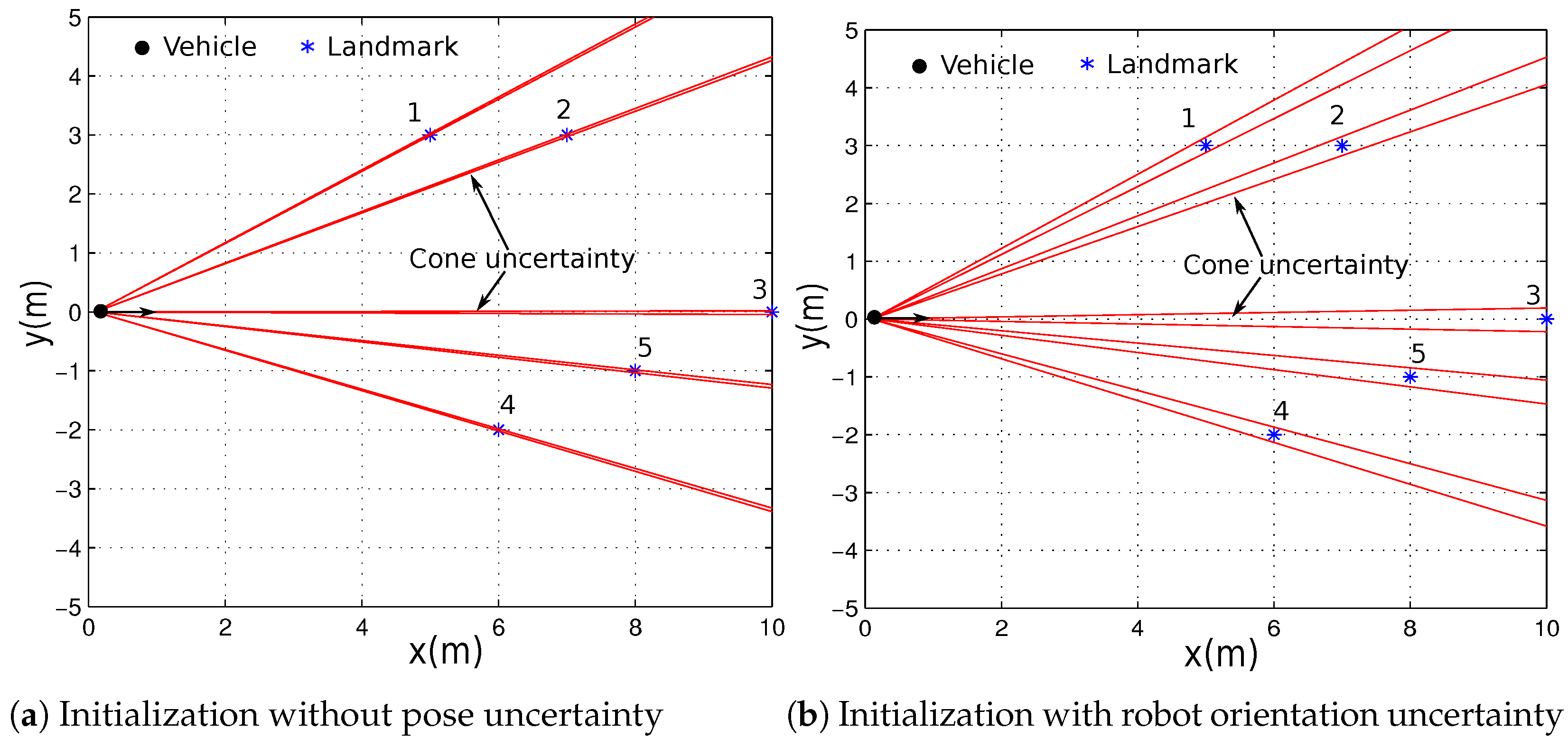
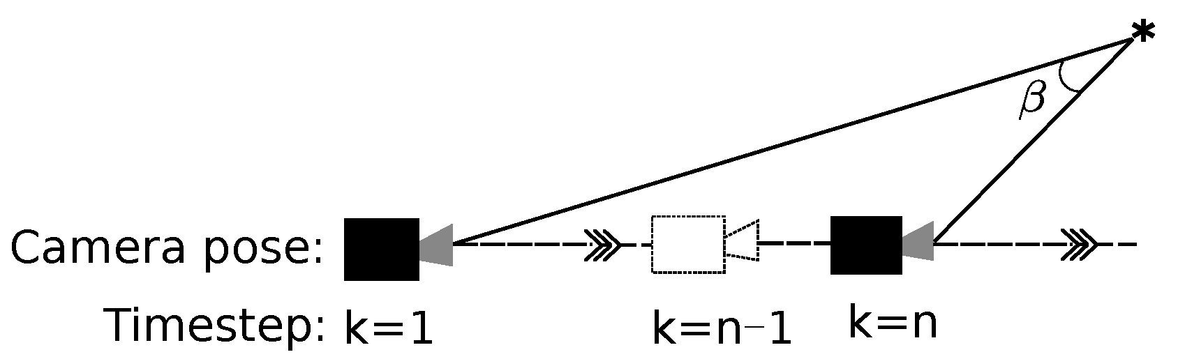
3.4.2. Undelayed Landmark Initialization

The interval-based parameterization enables us to initialize new landmarks immediately and consistently when the landmark is first observed, namely, undelayed initialization. The domain of each landmark’s parameters can be initialized as follows:

• ${([x_i],[y_i],[z_i])}^T={([x_k],[y_k],[z_k])}^T$: ${(x_k,y_k,z_k)}^T$ is the robot position, which is also the camera position for the sake of simplicity. When several landmarks are detected at the same time, they share the same parameter domains.
• $[{\alpha }_i]=[{\theta }_k]+[{\theta }_u]$, $[{\phi }_i]=[{\theta }_v]$: ${\theta }_k$ is the robot heading orientation, and ${\theta }_u$ and ${\theta }_v$ are the azimuth and elevation angles which are inferred from the pixel coordinate ${(u_i,v_i)}^T$ of the feature point related to the landmark ${\mathcal{L}}_i$. $u_i$ and $v_i$ correspond to an opening and elevation angle, defined by the pinhole model:

  $$\left(\begin{array}{c}[{\theta }_u]\\ [{\theta }_v]\end{array}\right)=\left(\begin{array}{c}[\arctan ]\left({\displaystyle \frac{[u_i]-[c_u]}{[f][k_u]}}\right)\\ [\arctan ]\left({\displaystyle \frac{[v_i]-[c_v]}{[f][k_v]}}·[\cos ]\left([{\theta }_u]\right)\right)\end{array}\right)$$

  (9)
  $(f,k_u,k_v,c_u,c_v)$ are the intrinsic parameters of the camera, where f is the focal length, $(c_u,c_v)$ is the principal point, and $(k_u,k_v)$ is the number of pixels per unit length. They can be determined by a camera calibration process.
• $[d_i]=[0,+\infty ]$: the unknown depth of the landmark; the initialization is guaranteed to contain the real value of $d_i$ for sure.

After the initialization process, the uncertainty of the landmark turns out to be an infinite cone, which incorporates the robot pose uncertainty, the observation uncertainty and the unmeasured depth uncertainty. The initialization result is complete and assuredly includes the real position of the landmark.

3.4.3. ICSP-Based Landmark and Robot’s Pose Estimation

A landmark observation refers to the pixel coordinates where the landmark is projected onto the image plane. Our approach models the estimation process as an ICSP. The prediction ${([u_i^{\mathrm{pre}}],[v_i^{\mathrm{pre}}])}^T$ of ith landmark on the image plane can be calculated by the pinhole camera model [29]:

$$[{\mathcal{L}}_i^c]=[R^{wc}]([{\mathcal{L}}_i]-[{\mathcal{X}}_k])$$

(10)

$${([u_i^{\mathrm{pre}}],[v_i^{\mathrm{pre}}])}^T\leftarrow \mathrm{CamProject}([{\mathcal{X}}_k],[{\mathcal{L}}_i^c])$$

(11)

The landmark estimation is formulated as shown above, offering several key advantages. For example, the nonlinear constraints are handled directly, without requiring linearization as in EKF-SLAM. Also, it provides guaranteed enclosures of all feasible solutions, ensuring consistency under bounded uncertainty. By using inclusion functions, nonlinear transformations are evaluated over interval domains in a way that guarantees the output intervals contain the true values. The $R^{wc}$ in Equation (10) represents the transformation matrix between the world frame and the camera frame. The interval domain intersection with observation ${([u_i^{\mathrm{obs}}],[v_i^{\mathrm{obs}}])}^T$ can be used to correct the bounding area prediction ${([u_i^{\mathrm{pre}}],[v_i^{\mathrm{pre}}])}^T$:

$$\left\{\begin{array}{c}[u_i^{\mathrm{pre}}]=[u_i^{\mathrm{pre}}]\cap [u_i^{\mathrm{obs}}]\hfill \\ [v_i^{\mathrm{pre}}]=[v_i^{\mathrm{pre}}]\cap [v_i^{\mathrm{obs}}]\hfill \end{array}\right.$$

(12)

Equation (12) established a relationship between the prediction and the observation of landmark ${\mathcal{L}}_i$, which introduces constraints on ${([u_i^{\mathrm{pre}}],[v_i^{\mathrm{pre}}])}^T$. It can be leveraged to contract the domains of both the robot pose $[{\mathcal{X}}_k]$ and landmark $[{\mathcal{L}}_i]$. Based on this formulation, an ICSP involving two primary constraints and nine variables can be constructed:

• A set of nine variables:

  $$V_k=\{x_k,y_k,{\theta }_k,x_i,y_i,z_i,{\alpha }_i,{\phi }_i,d_i\}$$

  (13)
• A set of nine domains:

  $$D_k=\{[x_k],[y_k],[{\theta }_k],[x_i],[y_i],[z_i],[{\alpha }_i],[{\phi }_i],[d_i]\}$$

  (14)
• A set of two top-level constraints:

  $$C_k={(C_k^1,C_k^2)}^T$$

  (15)

  $$\left\{\begin{array}{c}{C}_k^1\iff [u_i^{\mathrm{pre}}]=[u_i^{\mathrm{pre}}]\cap [u_i^{\mathrm{obs}}]\hfill \\ C_k^2\iff [v_i^{\mathrm{pre}}]=[v_i^{\mathrm{pre}}]\cap [v_i^{\mathrm{obs}}]\hfill \end{array}\right.$$

  (16)

For each detected landmark i at timestep k, an ${\mathrm{ICSP}}_k^i(V_k,D_k,C_k)$ can be generated. Each of these ICSPs can be individually addressed using a locally consistent ICP algorithm. As a result, the domains of each landmark parameters can be contracted. A key advantage is that all ICSPs are interconnected through the shared variables $x_k$, $y_k$ and ${\theta }_k$, representing the robot’s pose at the current timestep k. This correlation enables ICP algorithms to effectively perform joint contraction across the domains of all variables.

4. Theoretical Analysis and Evaluation of Mapping Consistency

The consistency is a key criterion for evaluating SLAM algorithms. A solution is generally considered consistent if the state estimates are unbiased and covariance accurately reflects the real mean squared error. In the context of interval analysis-based methods, consistency implies that the real value is reliably enclosed within the computed output interval. In this section, we will present the theoretical analysis on the consistency issue of our proposed iMonoSLAM algorithm.

4.1. Proposition of Theoretical Basis

Bounded-Error Measurement (BEM) concerns the measurement situations whose noises or errors are bounded and can be characterized by minimum and maximum bounds. It is a very common notation in practical engineering applications. On the one hand, sensor manufacturers typically specify the upper and lower bounds of measurement errors. On the other hand, engineers are always engaged in the problem of finding out the maximum and minimum values of some engineering parameters.

Definition 1.

A measurement equation is classically written as follows:

$$y_k=y_m\left(\mathbf{P}\right)+e_k,k=1,2,\cdots$$

(17)

where $y_k$ is the $k$th measurement corresponding to the state vector $\mathbf{P}\in {\mathbb{R}}^n$ and $e_k$ is the associated noise; $y_m\left(\mathbf{P}\right)$ is the perfect measurement value and k is the index of measurements.

Let us assume that $e_k\in [E]$ is always satisfied, and

$$[E]=\{e\in \mathbb{R}\mid -{ϵ}_r\le e\le {ϵ}_r\}$$

(18)

Indeed, in BEM the measurement noises are bounded with known limits, Equation (18) can be rewritten as follows:

$$\parallel e_k{\parallel }_{\infty }={ϵ}_r$$

(19)

with ${ϵ}_r$ as a known positive scalar and ${\parallel ·\parallel }_{\infty }$ representing the $\infty -norm$ (defined as $\parallel e_k{\parallel }_{\infty }=max\{|max\left(e_k\right)|,\mid min\left(e_k\right)\mid \}$).

Proposition 1.

Considering a single-input-single-output case, let $\overline{P}$ be a noise-free measurement of P ($P\in \mathbb{R}$, $\overline{P}=y_m\left(P\right)$, and a series of sensor readings $P_k$ with corresponding measurement noise $e_k$, such that

$$P_k=y_m\left(P\right)+e_k$$

(20)

Let $[E]=[-{ϵ}_r,{ϵ}_r]$ denote the bounded set (or interval) such that $e_k\in [E]$. One has

$$\underset{k=1}{\overset{\infty }{\cap }}\{P_k-[E]\}=\overline{P}$$

(21)

It means that if we have ∞ measurements then we can find the output value of a perfect (noise-free) sensor.

Proof. 

The measurement equation (Equation (20)) gives a one-to-one correspondence between the measurement space and the noise space. This correspondence defines a bijective map as follows: $P_k\to [E]$ given by $e_k=P_k-\overline{P}$. Let us rewrite Equation (21) as follows:

$$\underset{k=1}{\overset{\infty }{\cap }}\{(P_k-[E])-\overline{P}\}=0$$

(22)

or equivalently

$$\underset{k=1}{\overset{\infty }{\cap }}\{(P_k-\overline{P})-[E]\}=\underset{k=1}{\overset{\infty }{\cap }}\{e_k-[E]\}=0$$

(23)

Let us prove that the right term is equal to 0. By construction, suppose that

$$\underset{k=1}{\overset{\infty }{\cap }}\{e_k-[E]\}=\xi \mathrm{and}\xi \in \mathbb{R}$$

(24)

This supposition leads to the statement that $\forall k\in \{1,2,\cdots ,\infty \}$

$$\xi \in \{e_k-[E]\}$$

(25)

According to the interval arithmetic, $e_k-[E]=[e_k-{ϵ}_r,e_k+{ϵ}_r]$. Then Equation (25) can be written as

$$e_k-{ϵ}_r\le \xi \le e_k+{ϵ}_r$$

(26)

or

$$-{ϵ}_r\le e_k-\xi \le {ϵ}_r$$

(27)

By increasing the infinite possible value of k in Equation (27), we obtain, thanks to Equation (19),

$$\parallel e_k{\parallel }_{\infty }-\xi \le {ϵ}_r\mathrm{and}-{ϵ}_r\le -{\parallel e_k\parallel }_{\infty }-\xi$$

(28)

By using Equation (19),

$${ϵ}_r-\xi \le {ϵ}_r\mathrm{and}-{ϵ}_r\le -{ϵ}_r-\xi$$

(29)

Then we have the following:

$$-\xi \le 0\mathrm{and}0\le -\xi$$

(30)

Hence $\xi =0$ and the right expression of Equation (23) is certain to be zero:

$$\underset{k=1}{\overset{\infty }{\cap }}\{(e_k-[E])\}=0$$

(31)

Therefore

$$\underset{k=1}{\overset{\infty }{\cap }}\{P_k-[E]\}=\overline{P}$$

(32)

□

Proposition 2.

Let f be an invertible function. $f:{\mathbb{R}}^m\to {\mathbb{R}}^n$, $\mathcal{D}$ ($\mathcal{D}\in {\mathbb{R}}^m$) is the definition domain of f, given N subsets of the domain $\mathcal{D}$ which are respectively denoted by $D_1,D_2,\cdots ,D_N$. One has

$$\underset{i=1}{\overset{N}{\cap }}\left(D_i\right)=f\left(\underset{i=1}{\overset{N}{\cap }}{D}_i\right)$$

(33)

Proof. 

Denote $S=\underset{i=1}{\overset{N}{\cap }}\left(D_i\right)$ where $i=1,2,\cdots ,N$. Consequently, $S\subseteq f\left(D_i\right)$, and because f is invertible we obtain the following:

$$f^{-1}\left(S\right)\subseteq f^{-1}\left(f\left(D_i\right)\right)⟺f^{-1}\left(S\right)\subseteq D_i$$

(34)

Because Equation (34) is true for $i=1,2,\cdots ,N$, we can infer that

$$f^{-1}\left(S\right)\subseteq \underset{i=1}{\overset{N}{\cap }}{D}_i$$

(35)

By construction, assume that

$$f^{-1}\left(S\right)=\widehat{D}\mathrm{and}\underset{i=1}{\overset{N}{\cap }}{D}_i=\{\widehat{D},D^{\ast }\}$$

(36)

with $D^{\ast }$ is a singleton, $\widehat{D}$ is a subdomain of $\underset{i=1}{\overset{N}{\cap }}{D}_i$, and $D^{\ast }\notin \widehat{D}$, such that Equation (35) is satisfied. Since $D^{\ast }\in \underset{i=1}{\overset{N}{\cap }}{D}_i$, we have $D^{\ast }\in D_i$ and $f\left(D^{\ast }\right)\in f\left(D_i\right)$ ($i=1,2,\cdots ,N$). With this we can obtain that

$$f\left(D^{\ast }\right)\in \underset{i=1}{\overset{N}{\cap }}f\left(D_i\right)=S$$

(37)

Applying $f^{-1}$ on Equation (37) we have

$$D^{\ast }\in f^{-1}\left(S\right)=\widehat{D}$$

(38)

This contradicts the assumption $D^{\ast }\notin \widehat{D}$. From Equation (35) we have

$$f^{-1}\left(S\right)=\widehat{D}=\underset{i=1}{\overset{N}{\cap }}{D}_i$$

(39)

Since f is invertible,

$$S=f(\underset{i=1}{\overset{N}{\cap }}{D}_i)$$

(40)

From the precondition, we also have

$$S=\underset{i=1}{\overset{N}{\cap }}f\left(D_i\right)$$

(41)

Finally, we can make the conclusion that

$$f(\underset{i=1}{\overset{N}{\cap }}{D}_i)=\underset{i=1}{\overset{N}{\cap }}f\left(D_i\right)$$

(42)

□

Corollary 1.

Let $\mathcal{H}$ be a measurement model $\mathcal{H}:{\mathbb{R}}^m\to {\mathbb{R}}^n$, $\mathbf{P}\in {\mathbb{R}}^{\mathbf{m}}$ is the state vector whose true state is $\overline{\mathbf{P}}$, and $\mathbf{y}\in {\mathbb{R}}^n$ is the sensor output corresponding to the state vector. The map between the state space and the measurement space is defined as

$${\mathbf{y}}_k=\mathcal{H}\left(\mathbf{P}\right)+{\mathit{e}}_k,k=1,2,\cdots$$

(43)

 where k is the index of measurement, and ${\mathit{e}}_k$ is the bounded noise of the measurement model and ${\mathit{e}}_k\in [\mathbf{E}]$. Suppose that $\mathcal{H}$ is an invertible function such that $\overline{\mathbf{y}}=\mathcal{H}\left(\overline{\mathbf{P}}\right)$ and $\overline{\mathbf{P}}={\mathcal{H}}^{-1}\left(\overline{\mathbf{y}}\right)$, one has

$$\underset{k=1}{\overset{\infty }{\cap }}{\mathcal{H}}^{-1}\{{\mathbf{y}}_k-[\mathbf{E}]\}\stackrel{a.s.}{⟶}\overline{\mathbf{P}}$$

(44)

It means that we can get the internal state of a system from an infinite series of noisy measurements.

Proof. 

Since $\mathcal{H}$ is invertible, ${\mathcal{H}}^{-1}$ is also an invertible function. According to Proposition 2:

$$\underset{k=1}{\overset{\infty }{\cap }}{\mathcal{H}}^{-1}\{{\mathbf{y}}_k-[\mathbf{E}]\}={\mathcal{H}}^{-1}\left(\underset{k=1}{\overset{\infty }{\cap }}\{{\mathbf{y}}_k-[\mathbf{E}]\}\right)$$

(45)

From Proposition 1, we have $\underset{k=1}{\overset{\infty }{\cap }}\{{\mathbf{y}}_k-[\mathbf{E}]\}\stackrel{a.s.}{⟶}\overline{\mathbf{y}}$, therefore

$$\underset{k=1}{\overset{\infty }{\cap }}{\mathcal{H}}^{-1}\{{\mathbf{y}}_k-[\mathbf{E}]\}\stackrel{a.s.}{⟶}{\mathcal{H}}^{-1}\left(\overline{\mathbf{y}}\right)=\overline{\mathbf{P}}$$

(46)

□

4.2. iMonoSLAM Mapping Consistency Statement

Following the definitions in Section 3.1, let $\mathbf{R}$ be the state vector which stacks the robot and landmark unknown parameters:

$$\mathbf{R}=\left[\begin{array}{c}{\mathcal{X}}_k\\ \mathcal{M}\end{array}\right]=\left[\begin{array}{c}{\mathcal{X}}_k\\ {\mathcal{L}}_1\\ {\mathcal{L}}_2\\ ⋮\\ {\mathcal{L}}_n\end{array}\right]$$

(47)

Each parameter in vector $\mathbf{R}$ is measured and estimated with the robot navigating the environment. The observation function for vector $\mathbf{R}$ can be expressed as (see Equation (6))

$${\mathcal{Z}}_k=\mathcal{H}\left(\mathbf{R}\right)+{\mathit{e}}_k$$

(48)

where ${\mathcal{Z}}_k$ is the measurement at time k, $\mathcal{H}(·)$ is the observation model, $\overline{\mathbf{R}}$ is the true state of $\mathbf{R}$, and ${\mathit{e}}_k$ is the corresponding measurement noise.

In our case, the observation at time k corresponding to the $i$th landmark depends only on the current robot pose state ${\mathcal{X}}_k$ and the particular landmark state ${\mathcal{L}}_i$. Thus the individual measurement function can be written as

$${\mathcal{Z}}_k^i=\mathcal{H}({\mathcal{X}}_k,{\mathcal{L}}_i)+{\mathit{e}}_k$$

(49)

Ideally, the observation function $\mathcal{H}(·)$ is invertible such that ${\mathcal{H}}^{-1}(·)$ can be defined (e.g., full observation which provides information about all degrees of the landmark’s state), then the state of the landmark can be estimated by the following:

$${\mathcal{L}}_i={\mathcal{H}}^{-1}({\mathcal{X}}_k,{\mathcal{Z}}_k^i)$$

(50)

However, in monocular vision, the measurement (image) does not contain the depth information of the observed landmark, which indicates that the observation model is irreversible. Consequently, prior knowledge (assumption) should be assigned to $d_i$ to render $\mathcal{H}(·)$ invertible. In our method, the unmeasured depth is initialized as $[0,+\infty ]$ which is a consistent prior as it includes all the feasible values of landmark depth. With such a prior, Equation (50) can be augmented to

$${\mathcal{L}}_i={\mathcal{H}}^{-1}({\mathcal{X}}_k,{\mathcal{Z}}_k^i,d_i)$$

(51)

Let $[\mathbf{E}]$ be a bounded set that represents the support of the measurement noise ${\mathit{e}}_k$. Since ${\mathcal{X}}_k$ is pre-estimated in the localization process (Section 3.3), and the prior $d_i$ is consistently initialized, then Corollary 1 can be used to prove the consistency of ${\mathcal{L}}_i$ as $k\to \infty$:

$$\underset{k=1}{\overset{\infty }{\cap }}{\mathcal{H}}^{-1}({\mathcal{Z}}_k^i-[\mathbf{E}])\stackrel{a.s.}{⟶}\overline{{\mathcal{L}}_i}$$

(52)

Equation (52) demonstrates that after multiple observations, the estimation of the landmark ${\mathcal{L}}_i$ will converge to its true position which is said to be consistent. Furthermore, the ICP technology we adopted takes no linearization or approximation on the system equations. As a result, the consistency of iMonoSLAM is maintained. This is a very important issue for robotic mapping applications, especially in the case where safety is a priority.

4.3. Proposition of Consistency-Evaluation Method

In this section, we propose the consistency-evaluation method for the interval analysis-based SLAM method, which will later be used to verify the consistency of our proposed iMonoSLAM algorithm. An estimation result is considered consistent if it contains the real value. To evaluate the consistency of the estimation, the interval error is defined as the difference between the estimated state’s upper and lower bounds and the corresponding reference value:

$$[{\psi }_k\left(\alpha \right)]=[{\underline{\alpha }}_k-{\alpha }_k^{\ast },{\overline{\alpha }}_k-{\alpha }_k^{\ast }]$$

(53)

where the interval $[{\alpha }_k]=[{\underline{\alpha }}_k,{\overline{\alpha }}_k]$ is the estimated state of variable $\alpha$ at timestep k and ${\alpha }_k^{\ast }$ refers to the corresponding reference or real value. Accordingly, the consistency criterion is formulated as follows:

$$0\in [{\psi }_k\left(\alpha \right)]⟺{\alpha }_k^{\ast }\in [{\alpha }_k]$$

(54)

The consistency criterion is used to assess the consistency of each component of vector variable $\alpha$. The estimation of $\alpha$ is considered consistent only if all components satisfy the consistency condition. The estimation accuracy can be evaluated by $w\left([{\psi }_k\left(\alpha \right)]\right)$.

Equation (53) can be employed to calculate the real-time interval error associated with each landmark’s state. To verify the consistency of the mapping process, it is required to test if all the landmark’s interval errors satisfy the consistency criterion at each timestep. We propose to define the landmark global minimal error as an interval whose upper and lower bounds are respectively defined as the minimum upper bound and maximum lower bound of all the interval errors related to each landmark estimation. Let us denote the interval error of the $i$th landmark by $[{\psi }_k\left({\mathcal{L}}_i\right)]=[{\underline{\psi }}_k\left({\mathcal{L}}_i\right),{\overline{\psi }}_k\left({\mathcal{L}}_i\right)]$. For n detected landmarks, the upper bound ${\Gamma }_u$ and lower bound ${\Gamma }_l$ of the landmark global minimal interval error at timestep k can be defined as follows:

$${\Gamma }_u\left(k\right)=\underset{1\le i\le n}{min}\{{\overline{\psi }}_k\left({\mathcal{L}}_i\right)\}$$

(55)

$${\Gamma }_l\left(k\right)=\underset{1\le i\le n}{max}\{{\underline{\psi }}_k\left({\mathcal{L}}_i\right)\}$$

(56)

The landmark global minimal interval error is given by $[E_k]=[{\Gamma }_l\left(k\right),{\Gamma }_u\left(k\right)]$. Following the consistency criterion, we can draw a conclusion that if $0\in [E_k]$, then the estimation result for all the landmarks is consistent at timestep k.

Proof. 

Denoting the interval error of landmark ${\mathcal{L}}_i$ ($i\in \{1,\cdots ,n\}$) by $[{\psi }_k\left({\mathcal{L}}_i\right)]$. From Equations (55) and (56), we know that

$${\underline{\psi }}_k\left({\mathcal{L}}_i\right)\le {\Gamma }_l\left(k\right)\mathrm{and}{\overline{\psi }}_k\left({\mathcal{L}}_i\right)\ge {\Gamma }_u\left(k\right)$$

(57)

Thus we have

$$[E_k]=[{\Gamma }_l\left(k\right),{\Gamma }_u\left(k\right)]\subset [{\psi }_k\left({\mathcal{L}}_i\right)]$$

(58)

If $0\in [E_k]$, then the statement $0\in [{\psi }_k\left({\mathcal{L}}_i\right)]$ is certain to be true, and the estimation of any landmark ${\mathcal{L}}_i$ is consistent. □

Similarly, if $0\in [E_k]$ is satisfied for all $k\in \{1,\cdots ,n\}$, then we can conclude that the mapping process is consistent all over the time.

5. Simulation Result of iMonoSLAM

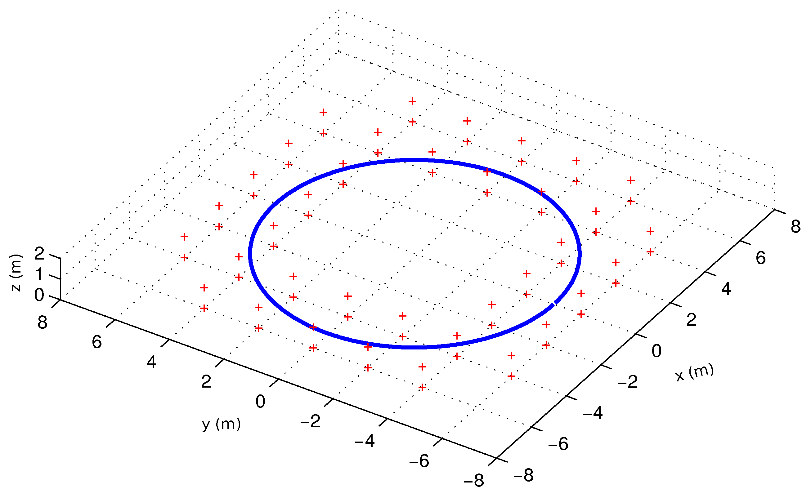
5.1. Experimental Setup

To obtain a quantitative evaluation of our proposed iMonoSLAM algorithm, extensive simulations have been performed. A square area (10 m × 10 m) is considered, where static landmarks are randomly positioned. The robot starts from the origin and moves around the environment. The camera model used in the simulation is defined as ($[f,k_u,k_v,c_u,c_v]=[40,8,8,320,240]$, pixel error: ≤1 pixel). The bounded error of the odometric sensor is set to be proportional to elementary displacement: $w\left([{\mathcal{U}}_k]\right)\le \gamma ·{\mathcal{U}}_k+\mathsf{\Gamma }$, where $\mathsf{\Gamma }=$ [0.1 mm, ${0.001}^{\circ }{]}^T$, ${\mathcal{U}}_k$ denotes the true odometric measurement and $\mathsf{\Gamma }$ refers to the steady system error. Then the UBB noises are characterized by the reference values adding the given maximum bounds:

$$[\alpha ]=[{\alpha }^{\ast }-ϵ·\Theta ,{\alpha }^{\ast }+(1-ϵ)·\Theta ]$$

(59)

where ${\alpha }^{\ast }$ is the reference value of variable $\alpha$ and $\Theta$ is the maximum imprecision, and $ϵ$ is an arbitrary number between 0∼1. When $ϵ=0.5$, the reference value is centered in the bounding interval. Firstly, the experiment is conducted without odometric noise to test the feasibility of estimating landmark uncertainty. This “no odometric noise” is then released in Section 5.3 and the following sections. When odometric noise is set to zero, the robot’s pose is assumed to be perfectly known, which leads to higher accuracy in pose estimation. As a result, the uncertainty in landmark estimation is reduced, and the interval contraction becomes more effective in the simulation.

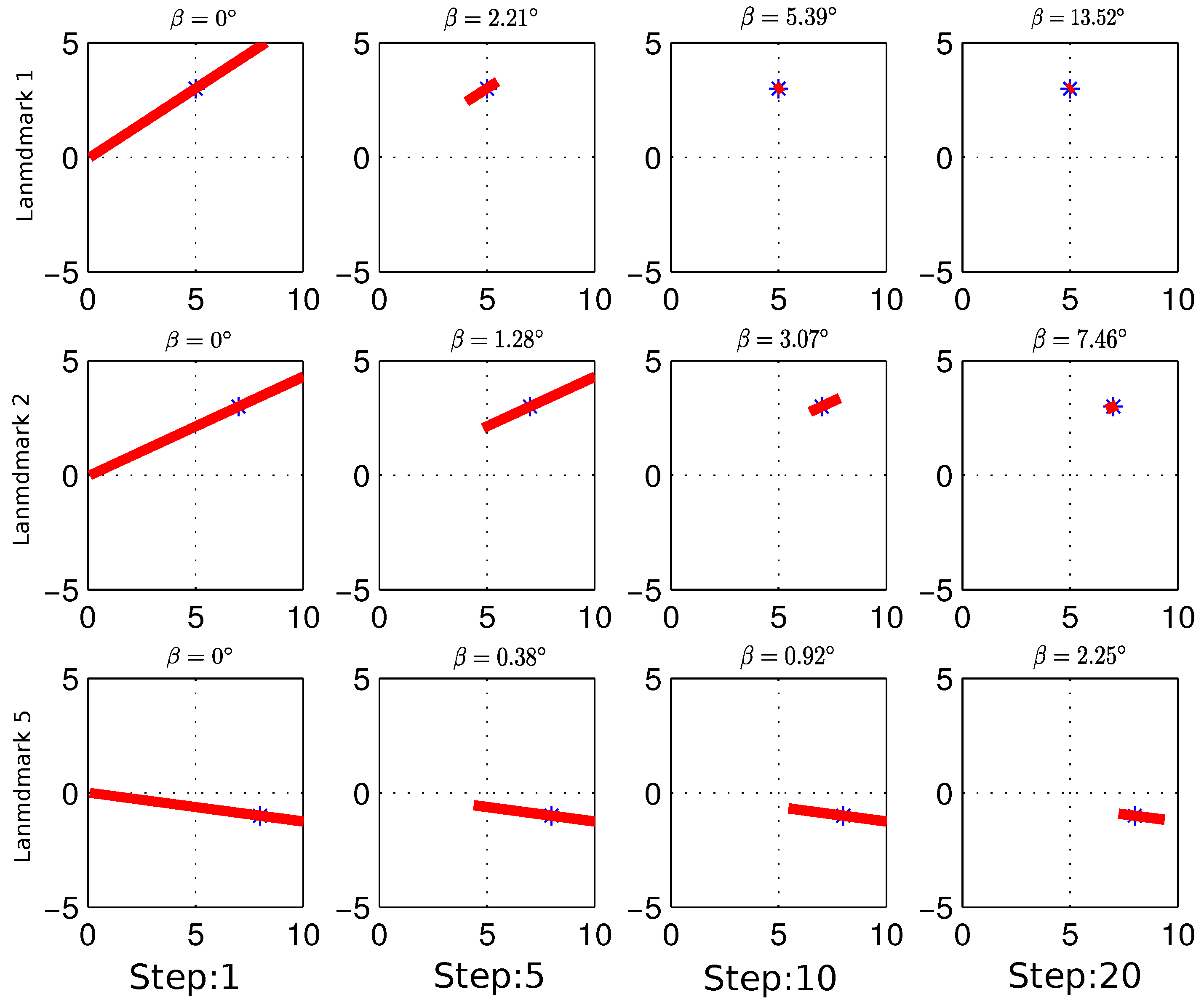
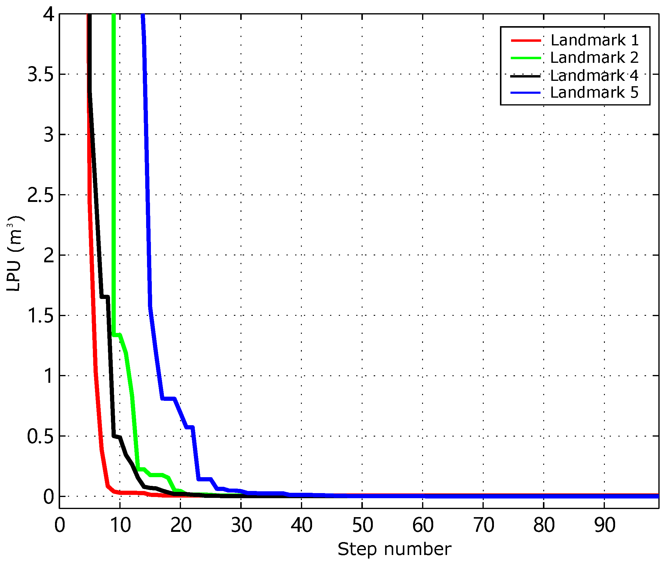
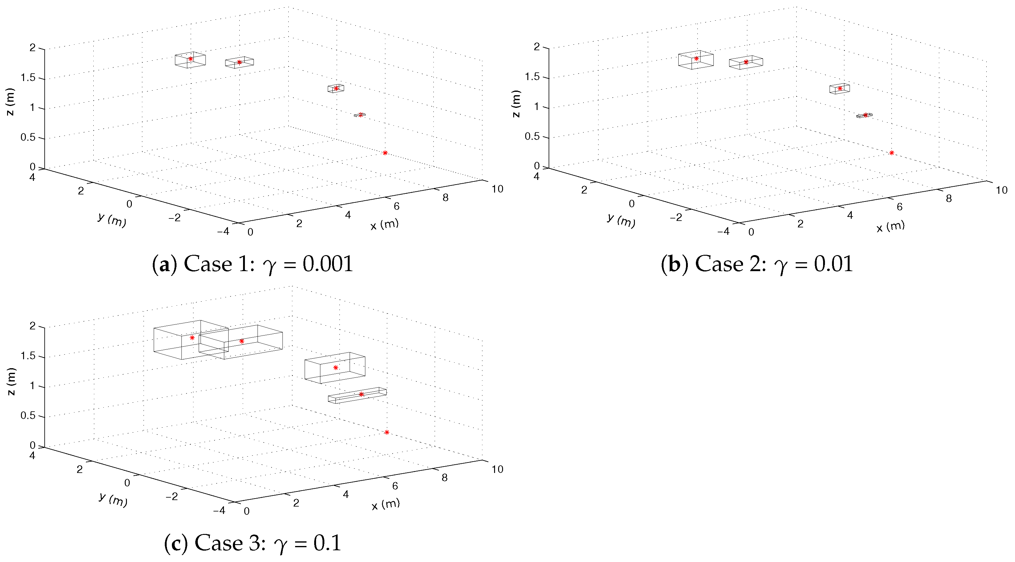
5.2. Landmark Initialization and Estimation

The landmark initialization process is started when a landmark is firstly detected. Figure 1a illustrates the initialization result of the five landmarks from the top view. In the absence of depth information, the uncertainty is initially modeled as an infinite cone. Given that the robot pose is assumed to be known precisely at initialization, the opening angles representing observation uncertainty are minimal. As shown in Figure 1b, the uncertainty cones are larger than the one without uncertainty. The combination of observation and pose uncertainties leads to the formation of cone uncertainty. Thanks to the UBB noise hypothesis, the resulting uncertainty cone at the initialization stage is guaranteed to enclose the true position of the landmark.

Repeated observations of the landmark from diverse angles with various parallax help reduce its cone uncertainty. By formulating and solving the relevant ICSP (see Section 3.4.3), the domain of the uncertainty cone can be contracted. As shown in Figure 2, the top-view progression of the uncertainty cones for landmarks 1, 2, and 5 is presented starting from initialization. Estimation results at timestep 1, 5, 10, and 20 are shown in each row. The parallax $\beta$ denotes the angular difference between the initial and current observations; see Figure 3. The landmark uncertainty estimation improves with time due to an increasing number of measurements, and an increase in the parallax angle results in more significant contraction of the landmark uncertainty. The infinite uncertainty will be significantly reduced while enough parallax observation is achieved. The uncertainty associated with landmark 3 remains unbounded over time because it lies along the x, and the parallax $\beta$ keeps zero during the horizontal translation movement. In this case, the depth information of this landmark will always be infinite, which leads to the un-contraction of the landmark’s uncertainty.

To depict the evolution of landmark position uncertainty (LPU) (m³), the 6-dimensional representation can be transformed into a global 3-dimensional point using Equation (8), and obtain ${(x_i,y_i,z_i)}^T$. Thus, the LPU is estimated as follows: $vol\left([{\mathcal{L}}_i]\right)=w\left([x_i]\right)\times w\left([y_i]\right)\times w\left([z_i]\right)$. With the initial depth of each landmark defined as $[0,+\infty ]$, the position intervals in x, y, and z are infinite, leading to an infinite LPU at the start. Following multiple observations taken at different times from varying viewpoints with sufficient parallax, the landmark position uncertainty is reduced. Figure 4 depicts the evolution of LPU associated with landmarks 1, 2, 4, and 5. Due to varying observation parallaxes, the uncertainty reduction for the four landmarks occurs at different times and is not simultaneous. However, they exhibit the same performance, with each landmark’s interval uncertainty being accurately propagated and decreasing exponentially during the robot’s movement.

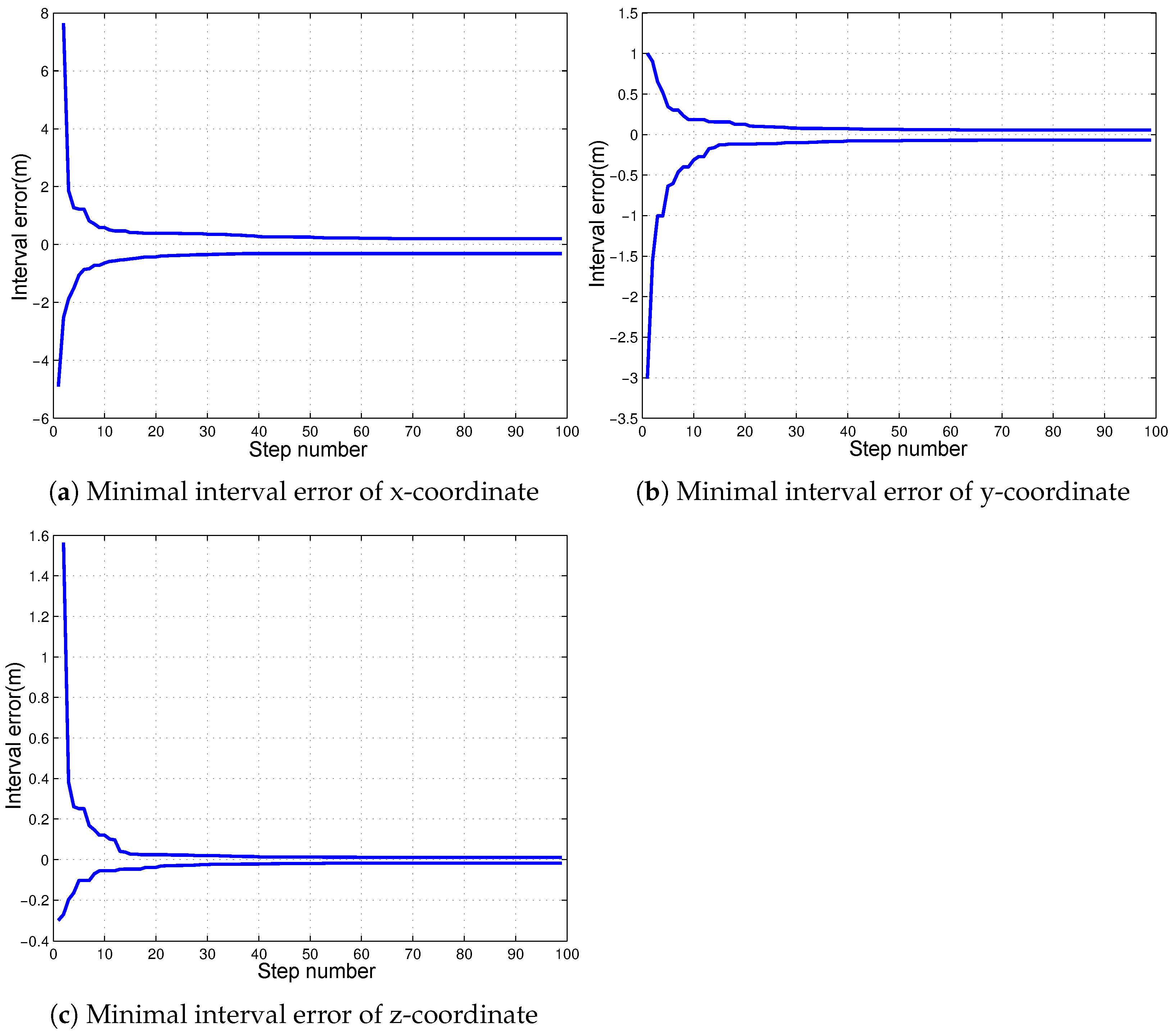
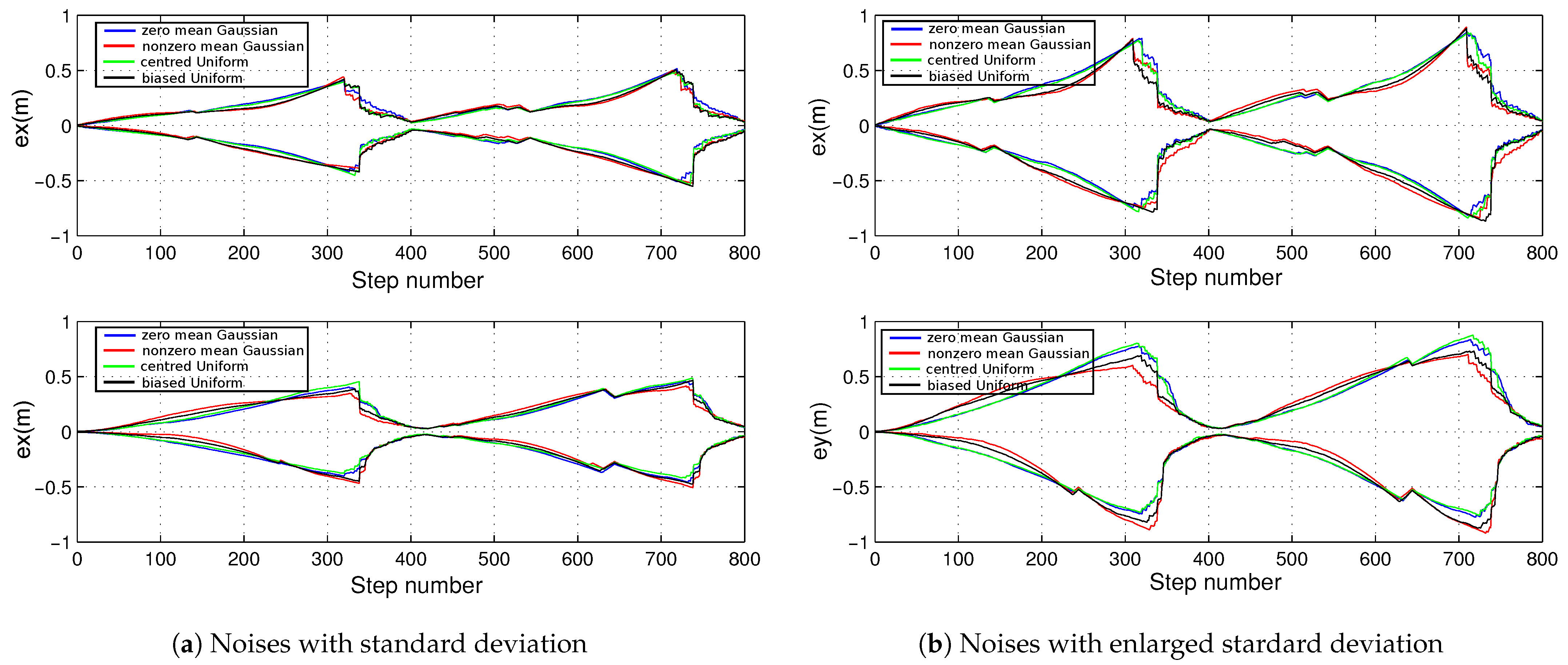
5.3. Analysis of the Effects of Odometric Noise

In real-world applications, odometric noise significantly affects the robot’s pose estimation and introduces considerable uncertainty. Bigger odometric noise will lead to a worse motion-estimation result (large localization box). Consequently, the initialization and estimation of landmark uncertainty will be affected. Section 5.2 has introduced the influence of robot pose uncertainty on initializing new landmarks. This section focuses on studying the influence of robot pose uncertainty on mapping accuracy.

We calculate, at each timestep, the robot position uncertainty and the mapping result (the mean landmark 3D position uncertainty) with different $\gamma$ values ($\gamma$ = 0.01, 0.1, and 0.2). As we can see in Figure 5a, bigger odometric noise leads to a relatively bigger localization uncertainty. As a result, the mapping accuracy decreases (see Figure 5b which is presented in a truncated form to show the difference more clearly). These findings highlight the strong correlation between landmark estimation accuracy and the robot’s pose uncertainty. Increased odometric error compromises pose accuracy, thereby reducing the precision of landmark estimates. The convergence rate of the mapping process is also influenced by the localization result: when $\gamma$ = 0.01, the map has almost reached its final precision around timestep $k=17$; when $\gamma$ = 0.2, the best precision is reached around $k=38$. This is reasonable, for the case $\gamma$ = 0.01, as the odometric noise is relatively small, and the uncertainty of robot localization increases more slowly than the case $\gamma$ = 0.2; thus, it could benefit a better landmark estimation. Thus the map could achieve a faster convergence. In Figure 5a, the localization uncertainty increases rapidly after timestep $k=70$. This is because after $k=70$, no landmark is observed except the one with infinite uncertainty (landmark 3).

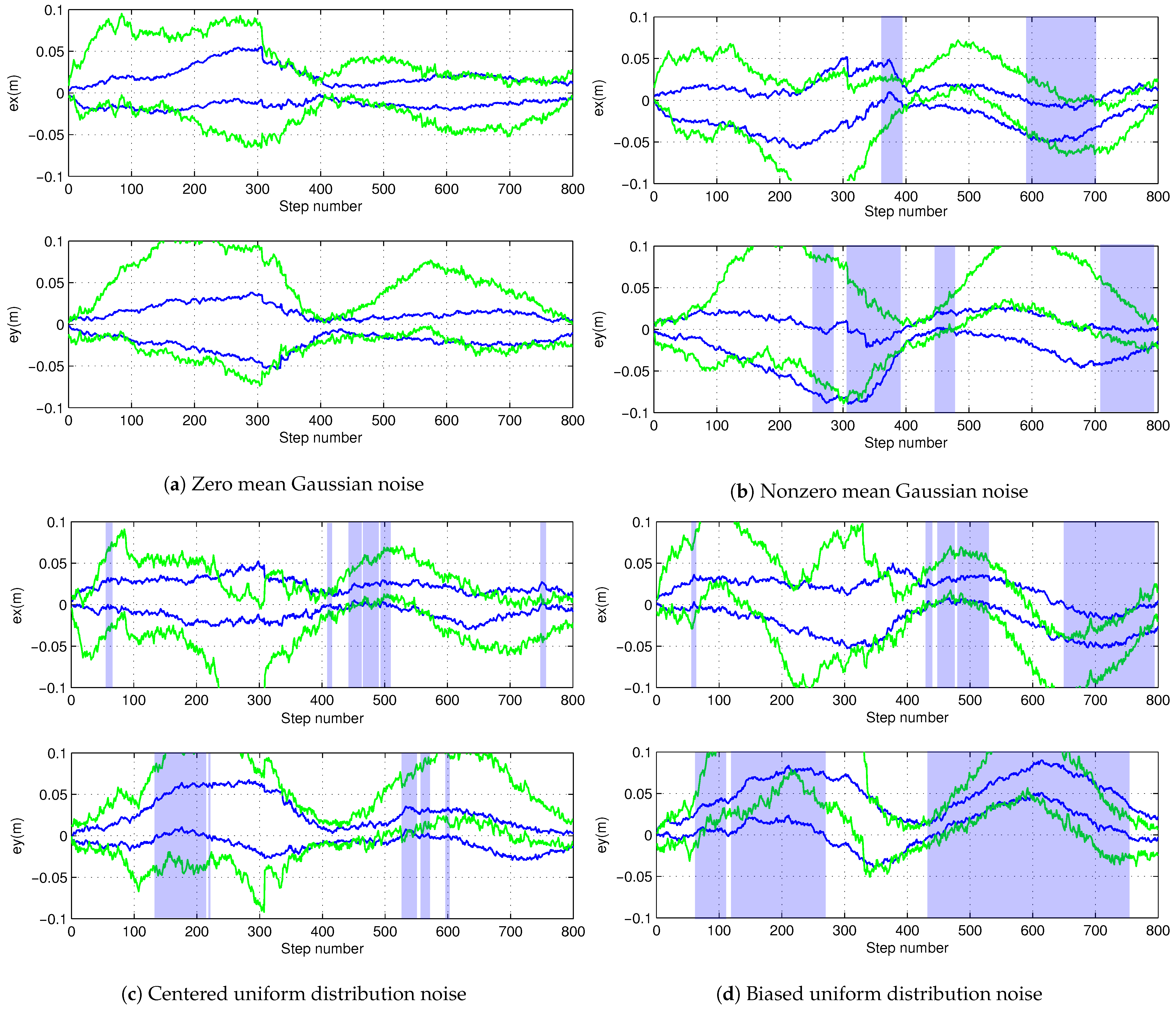
5.4. Consistency Validation of Mapping Result

We have claimed in Section 4.2 that the mapping result of iMonoSLAM is consistent. The estimated landmark position is represented by a bounding box. If the box encloses the landmark’s reference position, then the estimation result is said to be consistent. Figure 6 illustrates the final map created by iMonoSLAM under three experimental cases (different $\gamma$ values), together with the landmark reference position. It can be seen from the figure that all the landmark’s reference positions (red asterisk) are included by their estimated bounding box. The same results can be obtained by looking at the interval errors $E\left(\alpha \right)$ (see definition in Section 4.3, $\alpha \in \{x,y,z\}$) associated with each bounded landmark estimation). The results are presented in

Table 1. Interval error of estimated landmark position.

Noise Level	$\mathit{E}\left(\mathit{x}\right)$	$\mathit{E}\left(\mathit{y}\right)$	$\mathit{E}\left(\mathit{z}\right)$	0 ∈ $\mathit{E}\left(\mathit{\alpha }\right)$
$\gamma$ = 0.001	[−0.423, 0.338]	[−0.275, 0.218]	[−0.096, 0.071]	yes
	[−0.406, 0.373]	[−0.210, 0.169]	[−0.052, 0.048]	yes
	[−0.245, 0.212]	[−0.103, 0.095]	[0.048, 0.043]	yes
	[−0.223, 0.136]	[−0.061, 0.044]	[−0.013, 0.008]	yes
$\gamma$ = 0.01	[−0.495, 0.385]	[−0.247, 0.199]	[−0.111, 0.080]	yes
	[−0.492, 0.440]	[−0.210, 0.169]	[−0.062, 0.056]	yes
	[−0.312, 0.275]	[−0.125, 0.116]	[−0.058, 0.055]	yes
	[−0.319, 0.204]	[−0.069, 0.055]	[−0.017, 0.011]	yes
$\gamma$ = 0.1	[−1.045, 0.848]	[−0.646, 0.529]	[−0.219, 0.174]	yes
	[−1.258, 1.112]	[−0.571, 0.490]	[−0.148, 0.139]	yes
	[−0.938, 0.878]	[−0.330, 0.323]	[−0.161, 0.161]	yes
	[−1.194, 0.864]	[−0.156, 0.163]	[−0.055, 0.037]	yes

numerically. In three simulation cases, the interval errors of each landmark (landmark id = 1, 2, 4, 5) include zero value, showing that the mapping results are consistent.

The above results only prove that the final obtained map is consistent. To verify the consistency during the whole mapping process, we adopt the consistency-evaluation method proposed in Section 4.3. At each timestep, the global minimal interval errors regarding x-, y-, and z-coordinates are calculated. The result obtained under $\gamma =0.01$ is plotted in Figure 7. As we can see, the interval corridor includes the zero line during the entire navigation. Based on the statement in Section 4.3, we can conclude that the estimations for all the landmarks are consistent during the entire mapping process. The same results are obtained when conducting the simulation with different $\gamma$ values. Such results coincide with the theoretical analysis in Section 4.2 demonstrating that our proposed iMonoSLAM is a consistent approach.

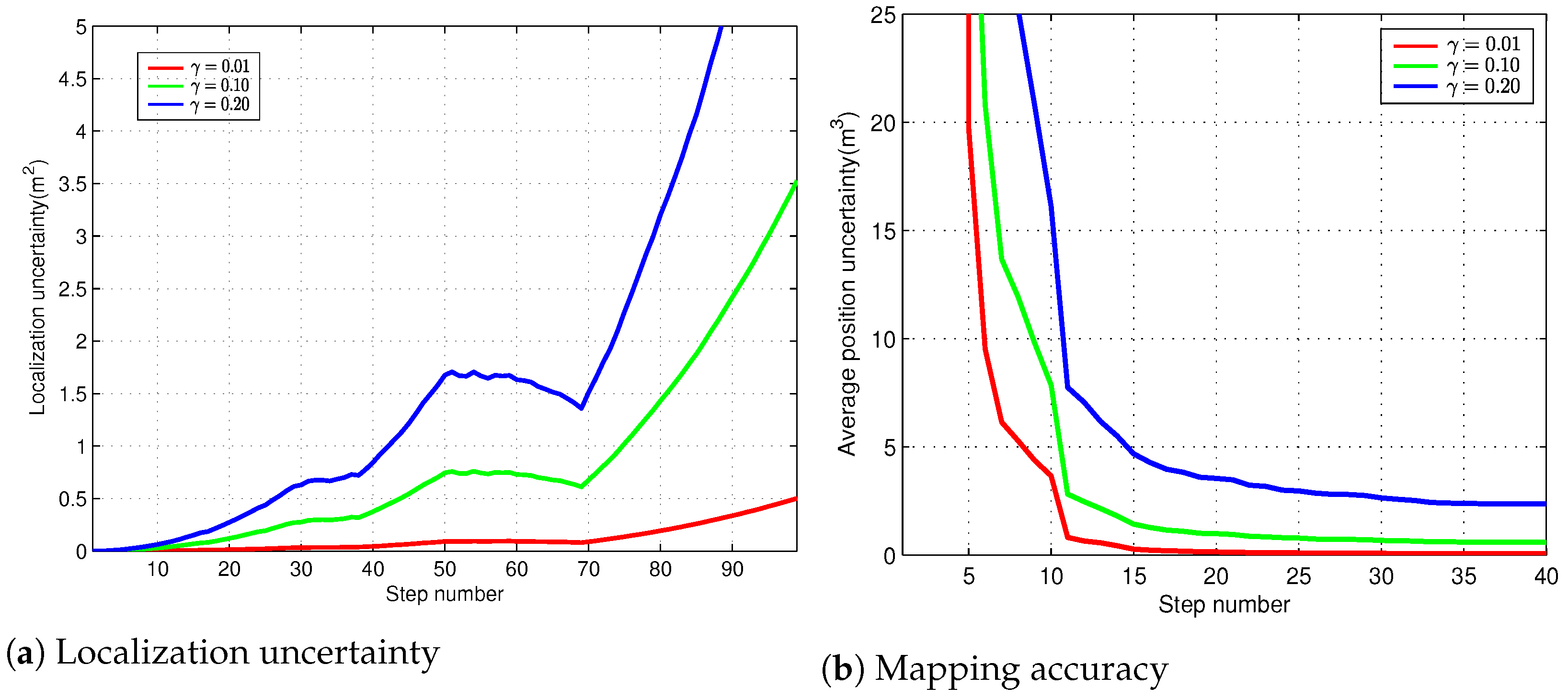
6. Comparison Between iMonoSLAM and EKF-SLAM

The feasibility of iMonoSLAM to provide consistent mapping results has been proven theoretically and shown experimentally in Section 4 and Section 5. In this section, we set up a more general case to compare the localization and mapping results with the classical EKF-SLAM algorithm. Constant displacement model (fixed linear and angular velocities) are considered for the robot, namely ${\mathcal{U}}_k={(\delta s_k,\delta {\theta }_k)}^T=(8$ cm, $0.9^{\circ }{)}^T$ such that it follows an anti-clockwise circle path around the environment on the $x-y$ plane. In total, 72 landmarks are randomly positioned around the path. Figure 8 is a snapshot of the environment, the red symbol ‘+’ represents the landmarks, and the blue curve denotes the reference path. The robot starts from point $(0,-5,0)$ and loops around the environment during 400 timesteps to come back to the starting point. The camera model used in the simulation is the same as the one introduced in Section 5.

Two normal types of probability density function (Gaussian $\mathcal{N}(\mu ,{\sigma }^2)$ and Uniform $U(a,b)$; the variance of the uniform distribution $U(a,b)$ is ${\sigma }^2={\displaystyle \frac{{(b-a)}^2}{12}}$. In the special case where $a=-b$ (centered uniform distribution), one has $b=\sqrt{3}\sigma$. Then the uniform distribution noise with a standard deviation $\sigma$ can be generated as $U(-\sqrt{3}\sigma ,\sqrt{3}\sigma )$.)) are considered to generate four sets of odometric noise: zero mean Gaussian noise, nonzero mean Gaussian noise ($\mu =0.2\sigma$), centered uniform distribution noise, and biased uniform distribution noise (bias $=0.2\sigma$). These noises are generated to have the same standard deviation (${\sigma }_s=0.03$ and ${\sigma }_{\theta }=0.003$). EKF-SLAM approximates all these noise distributions to Gaussian, whereas iMonoSLAM considers only the error bounds. For the sake of a fair comparison, when the noise of a parameter in EKF-SLAM is fed with a Gaussian distribution $\alpha \sim N(\mu ,{\sigma }^2)$, the bounded error support for iMonoSLAM will be characterized as three times the standard deviation ($3\sigma$), which corresponds to a 99.73% confidence level.

6.1. Localization Result Comparison

The robot follows two loops around the simulated environment. We calculate, at each time step, the interval error of the localization result of both algorithms. The output estimated localization of iMonoSLAM, which is a bounding area, has directly been used to compute the interval error for the coordinate x and y. For the EKF, we use the 3-sigma ellipsoids to define the imprecision area which encloses a probability concentration of 99.7%, then the bounds of the circumscribed rectangle are used to calculate the interval error [30]. A filter is considered effective if its corridor is thin and consistently contains the zero value, indicating that its uncertainty range encompasses the reference value.

Figure 9 and Figure 10 present the localization results obtained from executing EKF-SLAM and iMonoSLAM with the four generated odometric noises. Although the probability distribution of the input noise changes, the obtained localization results of iMonoSLAM are consistent: the interval error corridors always include the zero line (see Figure 9a). However, the localization consistency of the EKF-SLAM varies depending on the input noise, and only the zero mean Gaussian case turns out to be consistent. When the input noise is nonzero mean Gaussian or uniform distribution, EKF-SLAM shows some inconsistent results (the dark blue parts on the figure): the zero value lies outside the interval corridor at some instant. When the noise distribution is biased uniform, the localization result of EKF-SLAM shows huge inconsistencies. We enlarge the standard deviation (${\sigma }_s=0.09$ and ${\sigma }_{\theta }=0.009$) of the input noise to repeat the experiments. For iMonoSLAM, as the deviation of input noise increases, the localization uncertainty (the width of error corridor) increases (see Figure 9a), but the results are still consistent. For EKF-SLAM, the inconsistency becomes worse than previous results; see the green curves in each figure.

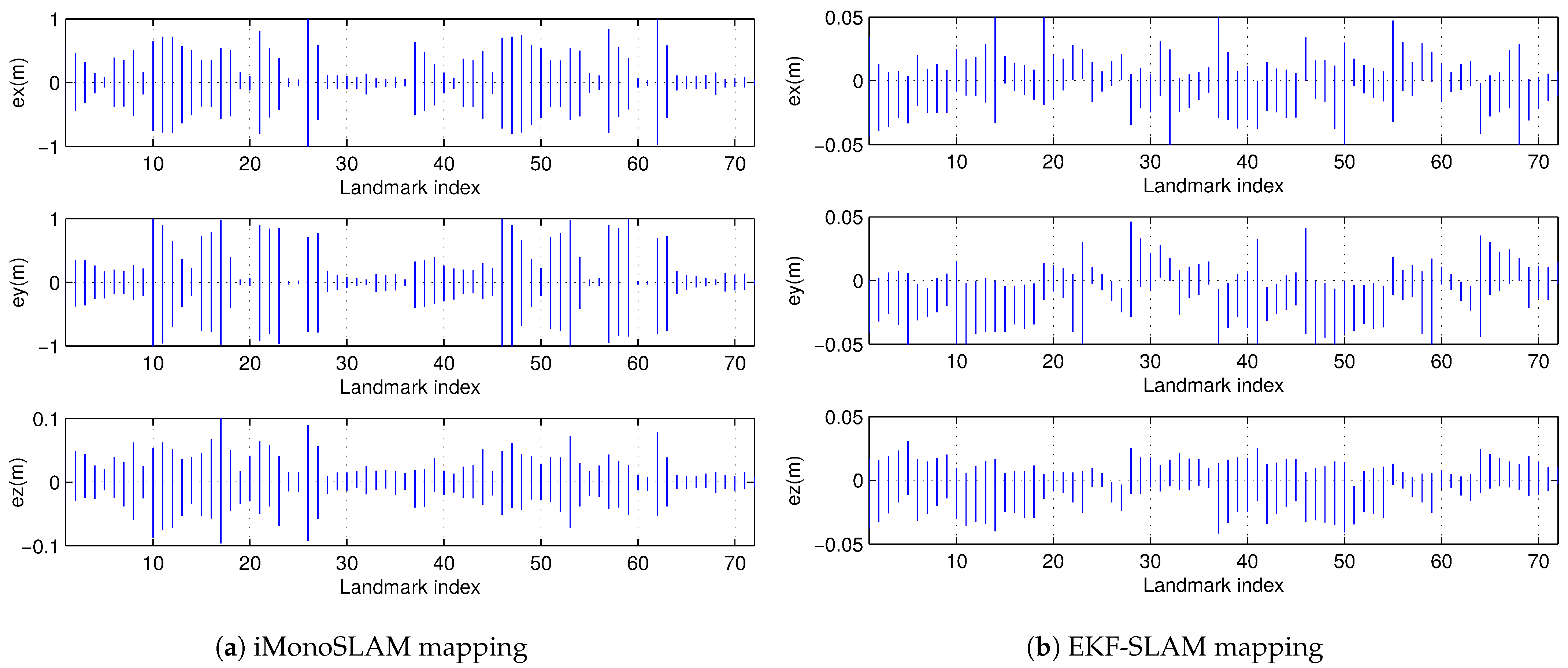
6.2. Mapping Consistency Comparison

In this section, we compare the mapping results of the two algorithms. At the end of the navigation, we utilize the same method to calculate the interval error concerning each landmark’s x-, y-, and z-coordinate for iMonoSLAM and EKF-SLAM. To visualize the result, the interval error associated with each landmark position is expressed in the figure by line-segments whose endpoints represent the lower and upper bound of the interval error (see Figure 11). If the line-segment intersects with the zero line, then the estimation of the corresponding landmark is consistent. Figure 11 shows an example of the results of iMonoSLAM and EKF-SLAM with nonzero mean Gaussian noise. As we can see the mapping result of iMonoSLAM is consistent, and all the line-segments go across the zero line. Conversely, for EKF-SLAM, the estimation of some landmarks is inconsistent.

Table 2. Number of inconsistent landmark estimations.

Algorithm	Zero Mean Gaussian	Nonzero Mean Gaussian	Centred Uniform	Biased Uniform
EKF-SLAM	0	18	6	17
	0	16	26	33
	0	6	3	7
iMonoSLAM	0	0	0	0
	0	0	0	0
	0	0	0	0

presents statistics of the inconsistent landmark estimation for the four different input noise; the consistency mapping is only achieved in the zero mean Gaussian noise case for EKF-SLAM, and for other noise cases, there are a lot of inconsistent estimations. This indicates that the mapping consistency of EKF-SLAM is not guaranteed. However, for our proposed iMonoSLAM, the estimation result depends only on the noise error bounds, and the consistency is guaranteed no matter what the noise distribution is. Thus, the statistics of inconsistent estimation are zero for the four experimental cases.

Such results demonstrate that the consistency of EKF-SLAM is only guaranteed in some special cases with strong requisites, i.e., zero mean Gaussian noise. In practical applications, the noise distribution for sensors are unknown, and only the maximum and minimum errors are provided by the sensor manufacturers, making the EKF-based method not feasible for practical implementation. To achieve consistent results in such scenarios, iMonoSLAM shows better performance than the EKF-SLAM to guarantee the consistency. The entire feasible region for the landmark (due to unobserved depth) is preserved and the box-based representation incorporates both sensor noise and robot pose uncertainty. In addition, the Interval Constraint Satisfaction Problems (ICSPs) are then iteratively solved to contract the box as new observations with parallax become available.

Calculating an average mapping imprecision of iMonoSLAM gives 0.79 m for x, 0.77 m for y, and 0.065 m for z. As the estimation of z depends on the observation elevation angle and is independent on the heading angle, it has higher accuracy than x and y. The estimation of x and y are affected by the robot’s pose state uncertainty. To obtain a better map, it is necessary to obtain a better estimation of the robot pose state.

7. Discussion

To deal with the consistency issue exposed in the SLAM literature, we present an interval analysis-based SLAM algorithm (iMonoSLAM) in this paper. The proposed method works in two essential steps: the motion step uses a bounded displacement model to integrate odometric data and the observation step processes the monocular vision observations by constructing and solving ICSPs with the ICP technique. The main contribution is that we present the theoretical analysis and proof of the mapping consistency of the proposed iMonoSLAM algorithm. Simulation results proved that the iMonoSLAM is able to achieve consistent mapping results on the basis that the sensor noise is bounded. Comparisons are made with EKF-SLAM under different noise distributions. EKF-SLAM provides more optimistic estimation results but consistency is not maintained.

Although iMonoSLAM expresses a larger localization uncertainty (bounding box) than that of EKF-SLAM in the experiments, the results are stable and consistent during all the test. Therefore, further exploration of interval analysis-based SLAM methods is essential. The ability to deliver reliable results is vital for autonomous robotic applications, particularly in scenarios where safety is of paramount importance. Moreover, our proposed consistency evaluation method can also be applied to evaluate the consistency property of other interval analysis-based SLAM algorithms. In future work, we would focus on developing and optimizing the ICP algorithms used in iMonoSLAM to elevate its performance in real applications with regards to the computational cost and estimation uncertainty. In addition, the multi-robot collaboration in dealing with the unbounded uncertainty would be explored.

8. Conclusions

In this paper, we introduced iMonoSLAM, an interval analysis-based SLAM algorithm designed to address the consistency issues commonly observed in SLAM literature. By integrating a bounded displacement model for motion estimation and utilizing ICSP techniques for monocular vision observations, iMonoSLAM ensures reliable and stable mapping under bounded sensor noise. Our theoretical analysis and proof confirm the mapping consistency of the proposed approach, distinguishing it from traditional probabilistic methods. Through simulations, we demonstrated that iMonoSLAM maintains consistency even under varying noise distributions, whereas EKF-SLAM tends to provide over-optimistic uncertainty estimates that compromise its consistency. While iMonoSLAM exhibits a larger localization uncertainty compared to EKF-SLAM, its ability to provide guaranteed localization and mapping results makes it a promising approach for safety-critical robotic applications.

References

1. Zhang, X.; Li, Y.; Cao, Z.; Lv, J.; Huang, Z.; Zhang, W. LiDAR-Inertial SLAM with DEM-driven Global Constraints for Planetary Rover Exploration. Int. Arch. Photogramm. Remote Sens. Spat. Inf. Sci. 2024, XLVIII-3-2024, 615–621. [Google Scholar] [CrossRef]
2. Teng, S.; Mueller, M.W.; Sreenath, K. Legged Robot State Estimation in Slippery Environments Using Invariant Extended Kalman Filter with Velocity Update. In Proceedings of the 2021 IEEE International Conference on Robotics and Automation (ICRA), Xi’an, China, 30 May–5 June 2021; pp. 3104–3110. [Google Scholar] [CrossRef]
3. Steuernagel, S.; Baum, M. Extended Object Tracking by Rao-Blackwellized Particle Filtering for Orientation Estimation. IEEE Trans. Signal Process. 2025, 73, 2590–2602. [Google Scholar] [CrossRef]
4. Tian, C.; Hao, N.; He, F. T-ESKF: Transformed Error-State Kalman Filter for Consistent Visual-Inertial Navigation. IEEE Robot. Autom. Lett. 2025, 10, 1808–1815. [Google Scholar] [CrossRef]
5. Rozsypálek, Z.; Rouček, T.; Vintr, T.; Krajník, T. Multidimensional Particle Filter for Long-Term Visual Teach and Repeat in Changing Environments. IEEE Robot. Autom. Lett. 2023, 8, 1951–1958. [Google Scholar] [CrossRef]
6. Zhang, T.; Wu, K.; Song, J.; Huang, S.; Dissanayake, G. Convergence and consistency analysis for a 3-D invariant-EKF SLAM. IEEE Robot. Autom. Lett. 2017, 2, 733–740. [Google Scholar] [CrossRef]
7. Jamaludin, A.; Mohamad Yatim, N.; Mohd Noh, Z.; Buniyamin, N. Rao-blackwellized particle filter algorithm integrated with neural network sensor model using laser distance sensor. Micromachines 2023, 14, 560. [Google Scholar] [CrossRef] [PubMed]
8. Guo, B.; Guo, N.; Cen, Z. Obstacle Avoidance With Dynamic Avoidance Risk Region for Mobile Robots in Dynamic Environments. IEEE Robot. Autom. Lett. 2022, 7, 5850–5857. [Google Scholar] [CrossRef]
9. Han, W.; Jasour, A.; Williams, B. Non-Gaussian Uncertainty Minimization Based Control of Stochastic Nonlinear Robotic Systems. arXiv 2023, arXiv:2303.01628. [Google Scholar] [CrossRef]
10. Mohanty, S.; Naskar, A.K. Analysis of the Performance of Extended Kalman Filtering in SLAM Problem. In Proceedings of the 2019 6th International Conference on Control, Decision and Information Technologies (CoDIT), Paris, France, 23–26 April 2019; pp. 1031–1036. [Google Scholar] [CrossRef]
11. Ehambram, A.; Voges, R.; Brenner, C.; Wagner, B. Interval-based Visual-Inertial LiDAR SLAM with Anchoring Poses. In Proceedings of the 2022 IEEE International Conference on Robotics and Automation (ICRA), Philadelphia, PA, USA, 23–27 May 2022; pp. 7589–7596. [Google Scholar] [CrossRef]
12. Mustafa, M.; Stancu, A.; Delanoue, N.; Codres, E. Guaranteed SLAM–An interval approach. Robot. Auton. Syst. 2018, 100, 160–170. [Google Scholar] [CrossRef]
13. Wang, Z.; Lambert, A.; Zhang, X. Dynamic ICSP Graph Optimization Approach for Car-Like Robot Localization in Outdoor Environments. Computers 2019, 8, 63. [Google Scholar] [CrossRef]
14. Wang, Z.; Lambert, A. A Low-Cost Consistent Vehicle Localization Based on Interval Constraint Propagation. J. Adv. Transp. 2018, 2018, 2713729. [Google Scholar] [CrossRef]
15. Wang, Z.; Lambert, A. A reliable and low cost vehicle localization approach using interval analysis. In Proceedings of the IEEE International Conference on Dependable, Autonomic and Secure Computing, Athens, Greece, 12 August 2018; pp. 480–487. [Google Scholar]
16. Di Marco, M.; Garulli, A.; Lacroix, S.; Vicino, A. Set membership localization and mapping for autonomous navigation. Int. J. Robust Nonlinear Control 2001, 11, 709–734. [Google Scholar] [CrossRef]
17. Drocourt, C.; Delahoche, L.; Brassart, E.; Marhic, B.; Clérentin, A. Incremental construction of the robot environmental map using interval analysis. In Proceedings of the International Workshop on Global Optimization and Constraint Satisfaction, Lausanne, Switzerland, 18–21 November 2003; Springer: Lausanne, Switzerland, 2003; pp. 127–141. [Google Scholar]
18. Jaulin, L.; Kieffer, M.; Didrit, O.; Walter, E. Applied Interval Analysis: With Examples in Parameter and State Estimation, Robust Control and Robotics, 1st ed.; Springer: Berlin/Heidelberg, Germany, 2001. [Google Scholar]
19. Porta, J.M. CuikSlam: A kinematics-based approach to SLAM. In Proceedings of the IEEE International Conference on Robotics and Automation, Barcelona, Spain, 18 April 2005; pp. 2425–2431. [Google Scholar]
20. Jaulin, L. A nonlinear set membership approach for the localization and map building of underwater robots. IEEE Trans. Robot. 2009, 25, 88–98. [Google Scholar] [CrossRef]
21. Jaulin, L. Range-only slam with occupancy maps: A set-membership approach. IEEE Trans. Robot. 2011, 27, 1004–1010. [Google Scholar] [CrossRef]
22. Ou, Y.; Fan, J.; Zhou, C.; Cheng, L.; Tan, M. Water-MBSL: Underwater Movable Binocular Structured Light-Based High-Precision Dense Reconstruction Framework. IEEE Trans. Ind. Inform. 2024, 20, 6142–6154. [Google Scholar] [CrossRef]
23. Codreş, A.; Codreş, B.; Stancu, A. Guaranteed SLAM-A pure interval approach. In Proceedings of the International Conference on System Theory, Control and Computing, Sinaia, Romania, 19 October 2022; pp. 176–181. [Google Scholar]
24. Mohamed, M. Guaranteed SLAM–An Interval Approach. Ph.D. Thesis, University of Manchester, Manchester, UK, 2017. [Google Scholar]
25. Moore, R.E.; Kearfott, R.B.; Cloud, M.J. Introduction to Interval Analysis; Society for Industrial Mathematics: Philadelphia, PA, USA, 2009. [Google Scholar]
26. Khun, J.; Schmidt, J. Interval Constraint Satisfaction: Towards Edge Acceleration. In Proceedings of the 2022 11th Mediterranean Conference on Embedded Computing (MECO), Budva, Montenegro, 7–11 June 2022; pp. 1–4. [Google Scholar] [CrossRef]
27. Cleary, J.G. Logical arithmetic. Future Comput. Syst. 1987, 2, 125–149. [Google Scholar]
28. Xu, W.; Pan, Y.; Chen, X.; Ding, W.; Qian, Y. A Novel Dynamic Fusion Approach Using Information Entropy for Interval-Valued Ordered Datasets. IEEE Trans. Big Data 2023, 9, 845–859. [Google Scholar] [CrossRef]
29. Hartley, R.; Zisserman, A. Multiple View Geometry in Computer Vision; Cambridge University Press: Cambridge, UK, 2003. [Google Scholar]
30. Kueviakoe, K.; Wang, Z.; Lambert, A.; Frenoux, E.; Tarroux, P. Localization of a Vehicle: A Dynamic Interval Constraint Satisfaction Problem-Based Approach. J. Sens. 2018, 2018, 3769058. [Google Scholar] [CrossRef]
Figure 1. Landmark initialization.
Electronics 14 02966 g001
Figure 2. Interva l uncertainty evolution.
Electronics 14 02966 g002
Figure 3. Parallax observations.
Electronics 14 02966 g003
Figure 4. Landmark uncertainty evolution.
Electronics 14 02966 g004
Figure 5. Localization and mapping result with different γ value.
Electronics 14 02966 g005
Figure 6. Illustration of iMonoSLAM mapping result (the black bounding box represents the estimation uncertainty of each landmark).
Electronics 14 02966 g006
Figure 7. The minimal interval error of landmark estimation (the two blue lines represent the upper and lower bounds).
Electronics 14 02966 g007
Figure 8. Simulation environment.
Electronics 14 02966 g008
Figure 9. Localization results of iMonoSLAM under 4 different noise situations.
Electronics 14 02966 g009
Figure 10. Localization results of EKF-SLAM under 4 different noise situations: (1) blue curve: noises with standard deviation; (2) green curve: noise with enlarged standard deviation.
Electronics 14 02966 g010
Figure 11. Mapping result with nonzero mean Gaussian noise ( μ = 0.2 σ ).
Electronics 14 02966 g011