A Robust and Energy-Efficient Control Policy for Autonomous Vehicles with Auxiliary Tasks

Abstract

We present a lightweight autonomous driving method that uses a low-cost camera, a simple end-to-end convolutional neural network architecture, and smoother driving techniques to achieve energy-efficient vehicle control. Instead of directly constructing a mapping from raw sensory input to the action, our network takes the frame-to-frame visual difference as one of the crucial inputs to produce control commands, including the steering angle and the speed value at each time step. This choice of input allows highlighting the most relevant parts on raw image pairs to decrease the unnecessary visual complexity caused by different road and weather conditions. Additionally, our network achieves the prediction of the vehicle’s upcoming control commands by incorporating a view synthesis component into the model. The view synthesis, as an auxiliary task, aims to infer a novel view for the future from the historical environment transformation cue. By combining both the current and upcoming control commands, our framework achieves driving smoothness, which is highly associated with energy efficiency. We perform experiments on benchmarks to evaluate the reliability under different driving conditions in terms of control accuracy. We deploy a mobile robot outdoors to evaluate the power consumption of different control policies. The quantitative results demonstrate that our method can achieve energy efficiency in the real world.

1. Introduction

Traditional research studies in autonomous driving rely on diverse devices, e.g., LiDAR, radar systems, etc., to control their driving motion using SLAM (Simultaneous Localization and Mapping) [1,2,3] methods in complex environments. However, these sensing devices are extremely costly. For example, Autoware [4] and Apollo [5] represent two major open-source autonomous driving systems. These systems utilize extensive hardware sensors to acquire road scene data, including 64-beam or 16-beam LiDAR, millimeter-wave radar, GNSS + IMU integrated positioning, and multiple cameras with varied configurations. This results in relatively high hardware costs and complex system architectures for such solutions. In addition, it is difficult to synchronize and fuse different sensor readings in view of engineering. Recent years have witnessed the rapid advancement of autonomous driving thanks to computer vision technologies and deep learning models.

Meanwhile, vision devices have advantages in versatility and are easy to integrate with external systems. As a consequence, vision-based autonomous driving with deep learning models has gradually become a mainstream method in recent years. For example, researchers tend to deploy devices to simultaneously capture the visual information and the driving control signals, e.g., steering angle, throttle, etc. These recordings are then used to train deep learning models in order to achieve autonomous driving control according to different visual inputs.

In general, the task of training a control model to physically drive a car in a diverse set of environments has been approached either through behavior reflex learning [6,7,8,9], perception-based approaches [10,11,12], or a combination of the two. Though the perception-based approaches, i.e., mediated perception and direct perception, have become the trend, we believe that behavior reflex approaches still have the potential ability to handle complexity when driving in the real world. The goal of this paper is to explore possible solutions for designing a control policy for small mobile platforms (e.g., AGVs, inspection robots) based on behavior reflex learning to demonstrate improvements in energy efficiency in diverse environments. To achieve this, we introduce two auxiliary tasks into our autonomous driving method, which include the use of frame-to-frame difference images (FDIs) as input, and a view synthesis component as a visual encoder to assist in the creation of vehicle control policy. Specifically, event-based vision sensors [13,14] are designed according to biological neural systems, and research [15,16] has shown that learning-based approaches can benefit from the sensory input of event cameras in motion estimation and self-driving tasks. We hereby use FDIs as part of the visual input to train our autonomous driving model, as shown in Figure 1.

Traditional Difference Image methods compute pixel variations through image subtraction. In contrast, the proposed frame-to-frame difference image (FDI) method incorporates event camera operational dynamics to capture spatiotemporal variation patterns from vehicle movements. These selectively activated pixels—corresponding to motion boundaries and geometrically discontinuous structures (e.g., road marking discontinuities, vehicle contours)—demonstrate strong alignment with human visual attention mechanisms. By concentrating computational resources on parsing these critical geometric features, FDIs significantly mitigate the adverse effects of variable road/weather conditions while enhancing driving behavior prediction accuracy through optimized temporal information acquisition. In addition, research [17,18,19] illustrates that it is able to learn the correlation relationship between the visual appearance and the different angle of view. Inspired by this idea, we add a side task, namely upcoming-view synthesis, to help autonomous vehicles to sense what road scenes would look like for the next moment so as to improve the performance of driving smoothness. Combining with the above improvements, we finally built an autonomous driving architecture that is reliable under different driving conditions and is more energy-efficient than other traditional behavior reflex approaches. In summary, our contributions are as follows.

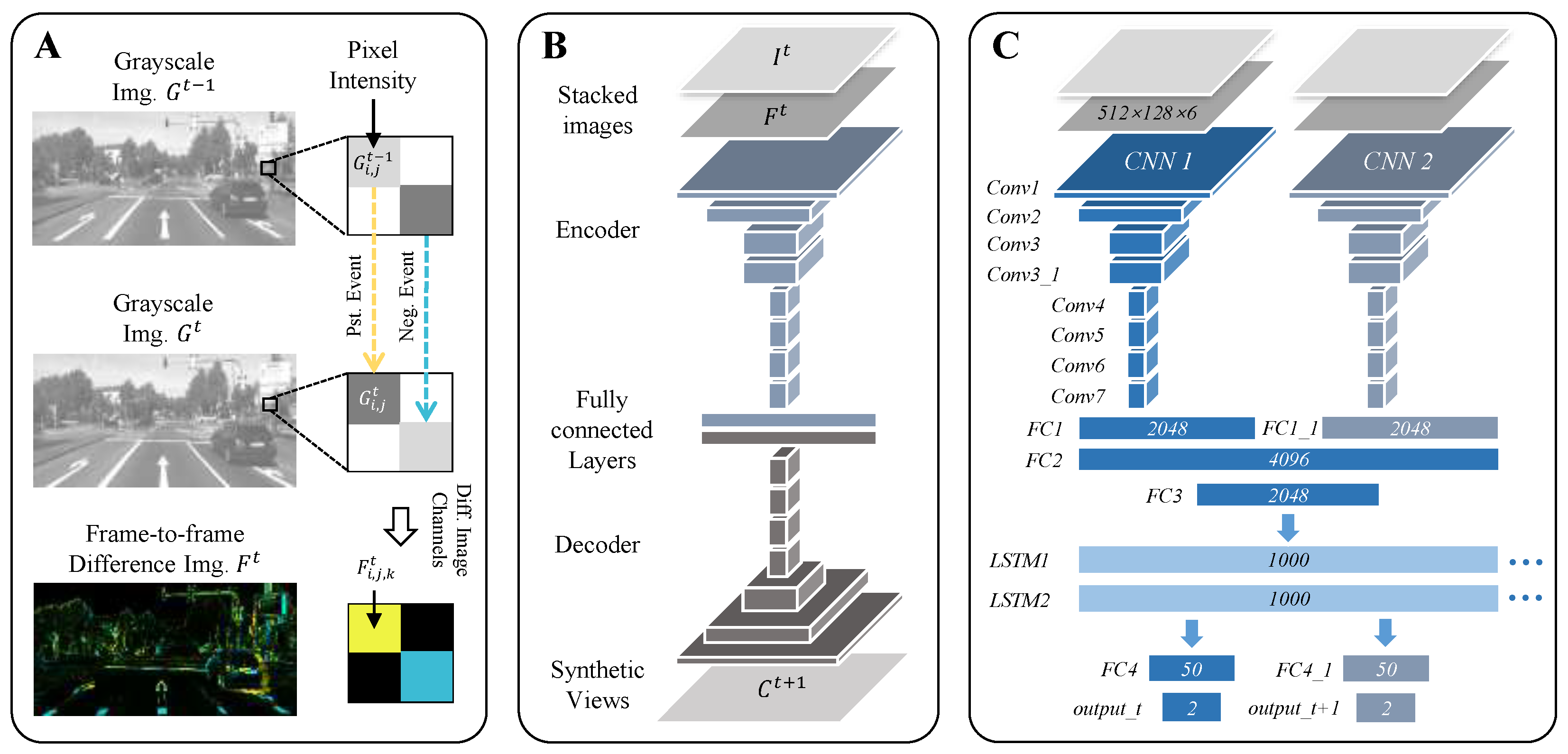
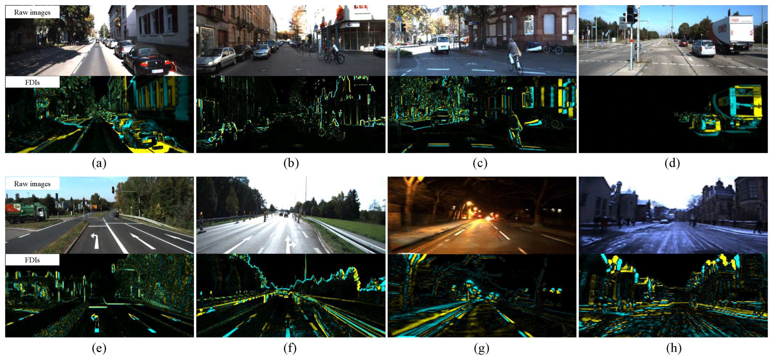
• We design a novel algorithm to create frame-to-frame difference images (FDIs) from raw visual sequences. Each FDI highlights the intensity change in the pixels caused by the change in vehicle movement. Taking FDIs as input can facilitate reliability when learning driving behaviors.
• We propose an end-to-end convolutional neural network to learn current and future driving controls based on the most distinct FDI features.
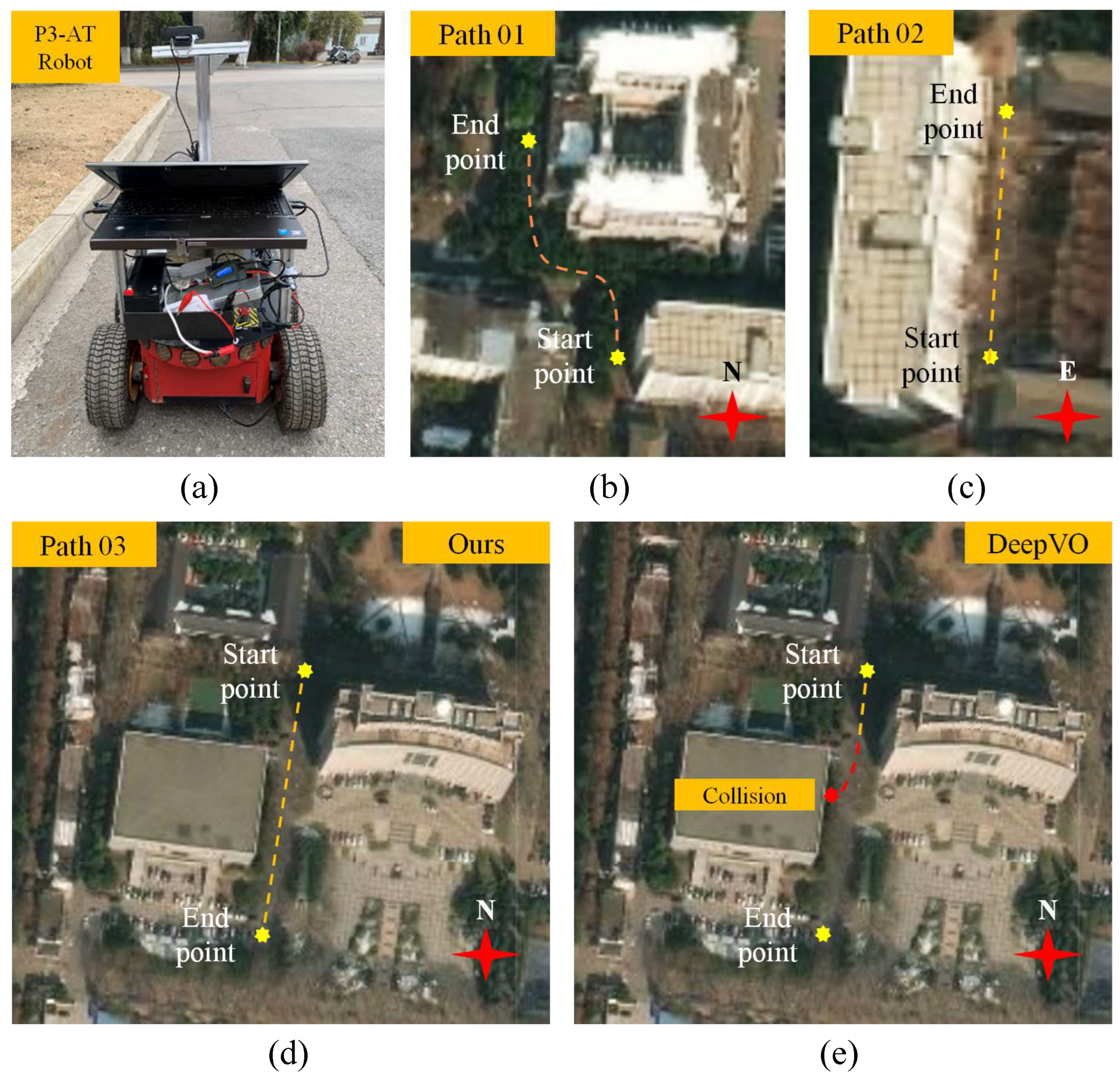
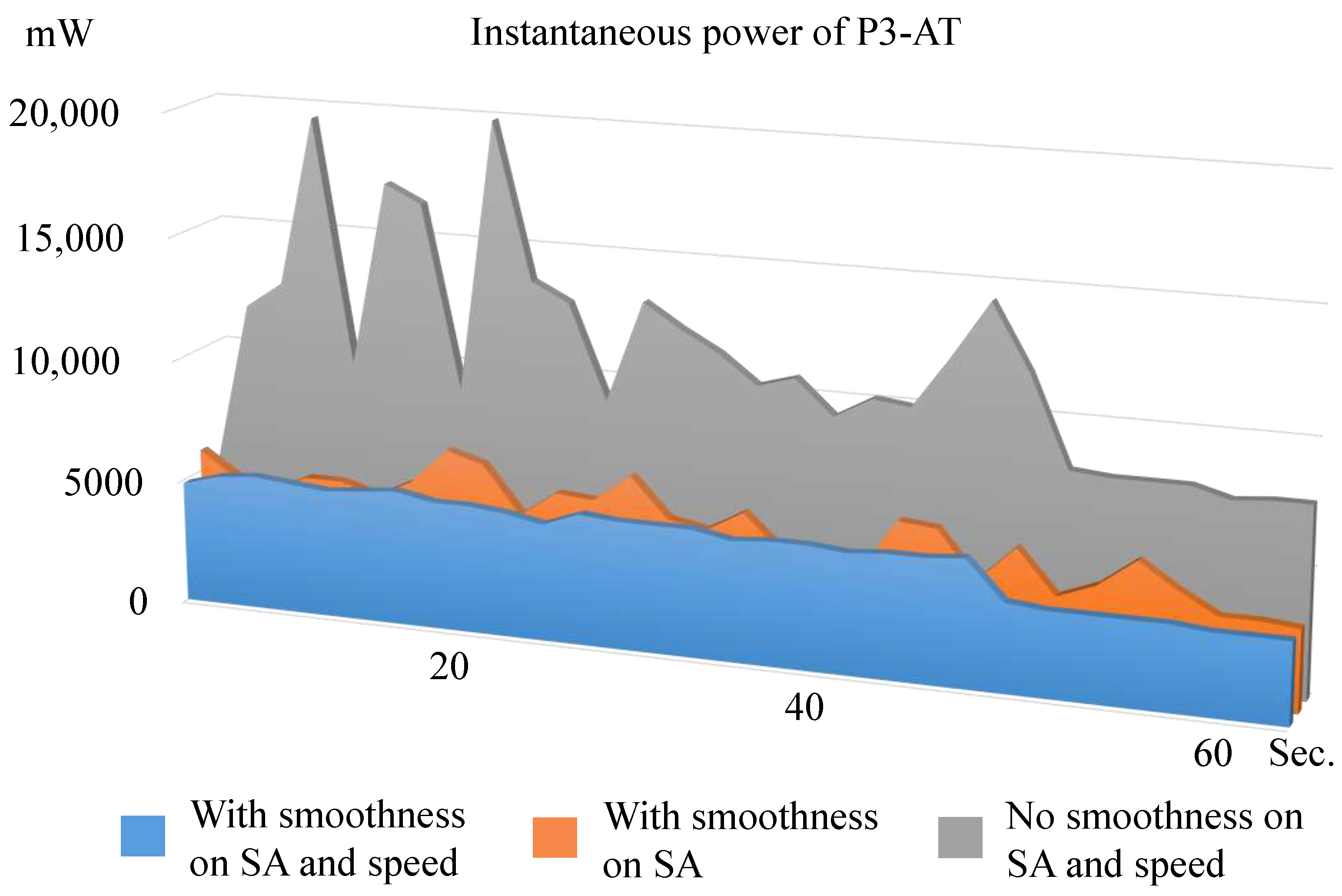
• We combine the control commands for the current and the upcoming time to achieve an energy-efficient control policy. In addition, we deploy a mobile robot in an outdoor environment to evaluate the performance of different control policies in terms of instantaneous power consumption.

This paper comprises six structured sections: Section 1 introduces fundamental autonomous driving approaches; Section 2 critically examines prior research relevant to our work. Section 3 provides a conceptual overview of our framework. Section 4 details the proposed pipeline, including two auxiliary tasks, the FDI generation principles, and the synthesis of the upcoming view. Section 5 evaluates the reliability of the system against industry-standard benchmarks. Finally, Section 6 concludes with key findings and future research directions.

2. Related Works

Recently, research has explored possible solutions for autonomous vehicles by using LiDAR [20,21] or stereo and monocular cameras [22,23] or combining multiple sensors [24]. In this paper, we focus on the solution by using pure visual sense as the input to achieve the autonomous driving, and this can be categorized into perception-based approaches and behavior reflex approaches.

Perception-based approaches [10] involve multiple sub-components for visual analyses, which are then combined into a world representation. These methods can be further divided into a mediated perception approach and a direct perception approach. Specifically, a mediated approach uses sub-components to implement recognition tasks [11] and includes but is not limited to traffic lights, traffic signs, etc. The direct perception approach uses a set of perception indicators to describe the driving state of the road and traffic. For example, C. Chen et al. [12] proposed a driving control system that adopts affordance indicators to represent road situations. Nevertheless, the above paradigms may add unnecessary complexity to the whole driving architecture, and the driving decisions reside in a relatively low dimension.

Behavior reflex approaches, such as [6], construct a direct mapping from the sensory input to a driving action. The models are generally built in an end-to-end manner, which has elegant architecture and great generalization performance. Most of them focus on tackling the weakness of behavior reflex learning by directly or implicitly regularizing intermediate representations of a driving model. Such methods can handle some complex or rare scenarios and scenarios that involve multi-agents. G. Costante et al. [25] focused on learning both the visual features and the ego-motion estimator via CNNs to perform accurate and robust estimation, in which they introduced the dense optical flow as the input. However, the CNN-based network architecture has limitations when handling sequential images. Recently, the RCNN based architecture has been proposed [7,8,26], which can perform the feature extraction and the sequential modeling at the same time. Authors in [7] proposed a recurrent convolutional neural network (RCNN) to achieve visual odometry, which has significant meaning that can refer to the autonomous driving. The authors adopt a CNN to learn the feature representation of the scene and an LSTM is deployed to model the variation in pose relations. However, these models learn correlation relations by the use of whole images rather than the most relevant parts, e.g., cars, traffic lines, etc. This may lead to relatively weak performance in reliability if we directly implement the autonomous driving model based on the above approaches. H. Xu and Y. Gao et al. [9] proposed an end-to-end approach to learn the vehicle motion models through video sequences from large-scale datasets and perform segmentation tasks during the learning of representation from raw pixels. Nevertheless, the accuracy of the actions may be affected when encountering the unsatisfied performance of the semantic segmentation. For recent learning-based autonomous driving approaches, the energy-efficient driving controls do not seem to be fully considered. J. Kim et al. [27] proposed an attention model to learn the visual explanations by highlighting relevant image regions which may imply a particular behavior. The authors utilize a single exponential smoothing method [28] which combines both the current and historical driving controls to improve the vehicle control performance. Z. Yang et al. [29] proposed a learning-based framework to predict vehicle control commands. Moreover, they achieve smooth control by applying a single exponential smoothing method on the predicted steering angles. It makes sense to achieve smoothness by using historical driving actions. However, this is not sufficient to achieve the demand of energy efficiency or safe driving unless future driving actions can be predicted.

Most existing methods directly feed raw image sequences into deep learning networks for training. However, adjacent frames may contain redundant pixel information. Therefore, an alternative approach draws inspiration from the operational principles of “event cameras” to pre-process input images. For example, such image preprocessing methods draw inspiration from event-based vision sensors [13,14,30] which are designed according to biological neural systems. The calculated image difference [31] is used to enhance the visibility of the respective input [32].

Meanwhile, research has shown that learning-based approaches can benefit from the sensory input of event cameras in motion estimation and self-driving tasks. For example, R. Ghosh et al. [15] achieved recognition and orientation estimation tasks with the use of a CNN. The data is acquired from a bio-inspired device that only responds to intensity changes. A. I. Maqueda et al. [16] adopted event-based devices to capture dynamic information from scenes. A network is then deployed to learn from the output of the event camera so as to perform steering angle prediction.

Additionally, some researchers employ auxiliary tasks to improve the performance of driving controls. The main idea comes from view synthesis, which originated from “mental rotation” [33], in which humans can predict possible views of objects or scenes with their known rotating directions. This ability allows drivers to predict what road scenes would look like at a new viewpoint [34,35]; hence, they can make driving decisions in advance to avoid redundant controls or to guarantee driving safety. Recent research in view synthesis provides multiple demonstrations to realize novel view synthesis through a learning-based approach [17]. For instance, M. Tatarchenko et al. [18] were able to generate the view of an unseen object by taking a single image and a new viewpoint as input. Here, a convolutional network is deployed to learn the correlation relationship between the visual appearance and the different angles of view. T. Zhou et al. [19] extended the above research to synthesize the object and scene structure from the desired new viewpoint.

3. Overview

This paper presents an energy-efficient autonomous driving solution using behavior reflex learning with two bio-inspired auxiliary tasks. First, frame-to-frame difference images (FDIs) apply event-based vision principles to capture vehicle-motion-induced pixel-level temporal variations. FDIs selectively emphasize critical geometric structures while suppressing noise, enhancing resilience to adverse conditions, as shown in Figure 2A. Second, an upcoming-view synthesis task employs multi-angle correlation learning to anticipate imminent scenes, as shown in Figure 2B. Both tasks are integrated into an end-to-end convolutional neural network architecture that processes two data streams (current state and future state) concurrently. Consequently, the model outputs dual predictions, which are immediate control and next-moment anticipatory control, as shown in Figure 2C. The synergistic integration of these tasks with the control policy achieves enhanced energy efficiency.

4. Methods

In this section, we first outline two main auxiliary tasks, the principle to create FDIs and the upcoming-view synthesis. We then present our autonomous driving model which incorporates with these two tasks to achieve robust driving control. Finally, the policy of energy-efficiency by combining recent and future control commands will be illustrated.

4.1. Frame-to-Frame Difference Image

We focus on creating a frame-to-frame difference image (FDI) to represent the variation between two nearby images in raw sequences, as shown in Figure 2A. Traditional approaches [36] create rough edges and show noise blobs on the difference images. We expect that an FDI should reveal the direction of intensity changes, also known as polarity, on pixels that are caused by the motion change, and the rest of the pixels, e.g., no-texture areas, should be removed as redundant. Taking the FDIs as input rather than the raw images allows the autonomous driving network to learn from the most important visual cues, which can guarantee reliability under different road and weather conditions. To achieve this, we first resize images in benchmarks to the dimension of $M\times N\times 3$ and convert the raw image $I^t$ into the grayscale one $G^t$ so as to compute the image difference by using the function below:

$$\begin{array}{c}\hfill N_{i,j}^t=\left|{\displaystyle \frac{\gamma G_{i,j}^t}{f_{std}}}-1.0\right|,\end{array}$$

(1)

$$\begin{array}{c}\hfill {\tilde{\mathit{D}}}_{\mathit{i},\mathit{j}}^{\mathit{t}}={\mathit{N}}_{\mathit{i},\mathit{j}}^{\mathit{t}}-{\mathit{N}}_{\mathit{i},\mathit{j}}^{\mathit{t}-1},\end{array}$$

(2)

where the grayscale image is denoted as ${\mathit{G}}^{\mathit{t}}:\mathsf{\Omega }\subset {\mathbb{R}}^{M\times N\times 1}$, and $\mathsf{\Omega }$ means the image domain. ${\mathit{G}}_{\mathit{i},\mathit{j}}^{\mathit{t}}$ is the intensity value of a pixel and $(i,j)$ is the coordinate of a pixel under the image coordinate. ${\mathit{N}}^{\mathit{t}}$ represents a normalized grayscale image that refers to normalization layer in [6], and the factor ${\mathit{f}}_{\mathit{std}}$ is set to 127.5 normally. We set a compensation factor $\gamma$ to correct the brightness change between two images, in which $\gamma$ is the ratio of the median value of the image intensity.

Finally, we use the image difference to create an FDI (which is denoted as $F^t$) according to the polarity (i.e., positive or negative) of each pixel’s intensity value.

$$\begin{array}{c}\hfill {\mathit{F}}^{\mathit{t}}=\left\{\begin{array}{cc}{\mathit{F}}_{\mathit{i},\mathit{j},0}^{\mathit{t}}=f_{std}|{\tilde{\mathit{D}}}_{\mathit{i},\mathit{j}}^{\mathit{t}}|,\hfill & \mathrm{if} {\tilde{\mathit{D}}}_{\mathit{i},\mathit{j}}^{\mathit{t}}>0\hfill \\ {\mathit{F}}_{\mathit{i},\mathit{j},1}^{\mathit{t}}=f_{std}|{\tilde{\mathit{D}}}_{\mathit{i},\mathit{j}}^{\mathit{t}}|,\hfill & \mathrm{if} {\tilde{\mathit{D}}}_{\mathit{i},\mathit{j}}^{\mathit{t}}<0\hfill \\ {\mathit{F}}_{\mathit{i},\mathit{j},2}^{\mathit{t}}=f_{std}{\mathit{N}}_{\mathit{i},\mathit{j}}^{\mathit{t}},\hfill & \mathrm{otherwise}.\hfill \end{array}\right.\end{array}$$

(3)

At this stage, we define two kinds of events, i.e., the positive event (if ${\tilde{D}}_{i,j}^t>0$) and the negative event (if ${\tilde{D}}_{i,j}^t<0$), to distinguish the polarity of the intensity change. Each kind of event is filled in an individual image channel so as to create a three-channel image ${\mathit{F}}^{\mathit{t}}$. As shown in Figure 3, we create FDIs by using image sequences in two typical benchmarks, i.e., the KITTI vision benchmark suite [37] and the Oxford RobotCar dataset [38]. The results illustrate that FDIs can provide the cleanest edges and polarity under different road and weather conditions. Specifically, fast or slow driving speed can be revealed on FDIs with different widths of contours, as in Figure 3a,b. When a vehicle is turning, the turning radius will lead to narrow and wide edges on an FDI, as in Figure 3c. Additionally, the driving actions, such as stop and move, can be observed clearly on FDIs, as shown in Figure 1 and Figure 3d. More importantly, FDIs are immune to the illumination changes in surroundings, in which the FDIs in Figure 3e–g remain clear contours when facing different levels of reflection light on road surfaces. In addition, FDIs are less affected by snow-covered road, as in Figure 3h, and this ability is important to ensure driving safety for autonomous vehicles under different weather conditions. Hence, we advocate for using FDIs rather than raw images as input to train the models in order to reliably predict driving actions.

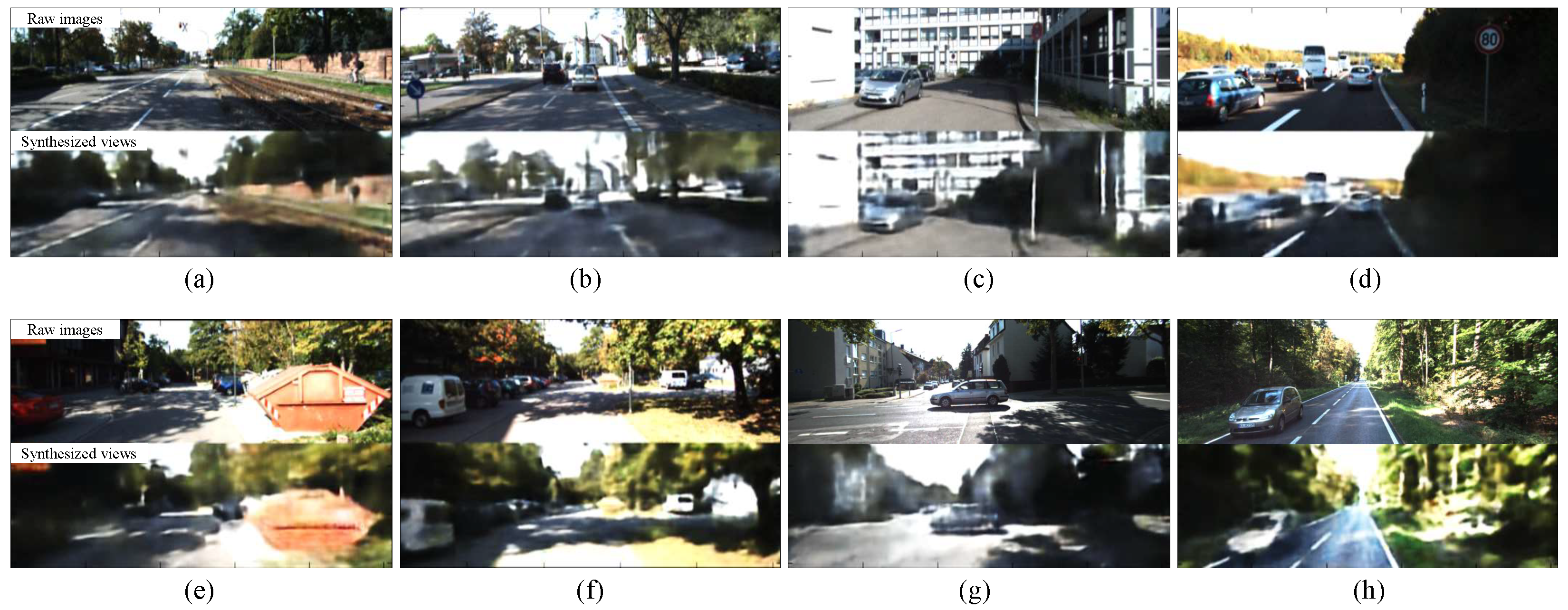
4.2. Upcoming-View Synthesis

With the frame-to-frame difference image to guarantee the accuracy and reliability of the prediction, the next goal is to predict the upcoming view by using historical information, in order to sense the change in driving conditions in advance. From observation, we found that the camera usually acquires data at a higher rate in which there are fewer changes between two adjacent frames during vehicle movement. Hence, it is possible to train a model to synthesize the upcoming view by using historical frames. In this paper, the upcoming view is defined as a synthetic image $C^{t+1}$ that can foreknow a novel view of the scene during driving. To achieve this, we design an upcoming-view synthesis network based on the encoder–decoder architecture in [19] to learn the hidden relationship between consecutive images by using stacked images (consisting of ${\mathit{I}}^{\mathit{t}}$ and ${\mathit{F}}^{\mathit{t}}$) as input and then output the upcoming view ${\mathit{C}}^{\mathit{t}+1}$. We minimize the following loss function to find out the optimal hyperparameters $\tau$ for the network:

$$\begin{array}{c}\hfill \tau =argmin{\sum }_{i,j,k}{∥I_{i,j,k}^{t+1}-C_{i,j,k}^{t+1}∥}_2,\end{array}$$

(4)

where $I_{i,j,k}^{t+1}$ and $C_{i,j,k}^{t+1}$ represent the pixel intensity of the raw image and the synthetic image, respectively. ${∥·∥}_2$ denotes the $L_2$ norm. Here, we use $L_2$ norm in experiments and we found $L_1$ norm could also obtain similar results. To learn the hyperparameters $\tau$ of our upcoming-view synthesis network, we first reshape the sensory input to 512 × 128 × 3 and then we create FDIs through consecutive image pairs and stack them together as a tuple <${\mathit{I}}^{\mathit{t}}$, ${\mathit{F}}^{\mathit{t}}$>. Finally, we feed the tuple into the model at each training iteration. The tuples are shuffled at the beginning to avoid model overfitting.

FDIs allow the model to learn the view change for the current time and predict the novel view for the next moment. Raw images provide rich textural information which can facilitate the synthesis of the upcoming view. The upcoming-view synthesis model is shown in Figure 2B. The architecture consists of a CNN that is modified from VGGNet [39]. The output of the CNN is then flattened and passed to two fully connected layers in which each layer has 2048 nodes. We then reshape the array of the last fully connected layer and feed it into a decoder that has seven up-sampling convolutional layers. Finally, the decoder outputs a synthetic image to predict what the scene would look like from the viewpoint of the camera at the next moment.

The upcoming-view synthesis model is trained and tested on benchmarks, and a part of the typical results is shown in Figure 4. The synthetic images can recover the surroundings, e.g., road surfaces, buildings, and traffic, when the vehicle is moving straight, as in Figure 4a–d. With the assistance of historical information, we can recover the views when the vehicle takes a quick turn, as in Figure 4e,f, which is much more challenging than straight driving. Additionally, vehicles with different moving directions can be predicted precisely, as shown in Figure 4g,h. We set upcoming-view synthesis as a side task to provide upcoming control commands of the autonomous driving network, which is explained in Section 4.3. Combining the current and upcoming control commands, the network can achieve driving smoothness, which directly relates to energy-efficiency (see Section 4.4).

4.3. Autonomous Driving Model

Our autonomous driving model is an end-to-end convolutional neural network architecture, as in [40], in which two CNNs are deployed to learn the representations of the current and upcoming views, respectively. The architecture of the proposed autonomous driving model is shown in Figure 2C. It stacks a raw RGB image and a frame-to-frame difference image as the input and processes them jointly through both $\mathit{CNN}1$ and $\mathit{CNN}2$. The configuration detail of each layer in a CNN is illustrated in

Table 1. Configuration of the CNN.

Layer	Receptive Field	Padding	Stride	Kernels	Feature Map Size
$Conv1$	7 × 7	3	2	64	256 × 64 × 64
$Conv2$	5 × 5	2	2	128	128 × 32 × 128
$Conv3$	5 × 5	2	1	256	64 × 16 × 256
$Conv{3}_{-}1$	3 × 3	1	2	256	64 × 16 × 256
$Conv4$	3 × 3	1	2	512	32 × 8 × 512
$Conv5$	3 × 3	1	2	512	16 × 4 × 512
$Conv6$	3 × 3	1	2	512	8 × 2 × 512
$Conv7$	3 × 3	1	2	512	4 × 1 × 512

.

Then, the feature maps are concatenated at the fully connected layers and passed forward to the LSTM module to generate the current and upcoming vehicle controls. The predicted vehicle controls will be combined together so as to eliminate the redundant operations. Also, these control commands can be used to design the safety constraints [41]. Each CNN has eight convolutional layers and we use the rectified linear unit (ReLU) as the activation function at each layer. Next, the parameters of $\mathit{CNN}2$ and $\mathit{FC}{1}_{-}1$ are initialized with the learned weights in the upcoming-view synthesis before joint training with $\mathit{CNN}1$.

In our autonomous driving model, we use the side task in Section 4.2 as an extra supervision to predict the upcoming control commands. We initialize $\mathit{CNN}2$ and $\mathit{FC}{1}_{-}1$ by using the fine-tuned weights of the encoder layers in the upcoming-view model, as shown in Figure 2B. Following the CNNs, three fully connected layers are deployed to concatenate the learned feature representation together and then are passed forward to an RNN to model the variation in vehicle controls. The RNN consists of two LSTM layers ($\mathit{LSTM}1$ and $\mathit{LSTM}2$), and each layer has 1000 hidden states. At last, two short fully connected layers ($\mathit{FC}4$ and $\mathit{FC}{4}_{-}1$) will output the current and upcoming control commands, which are ${\mathit{output}}_{\mathit{t}}$ and ${\mathit{output}}_{\mathit{t}+1}$, respectively. By taking two CNNs as encoders, our autonomous driving model is jointly trained to learn the feature representations of both the current and upcoming images through stacked input and then generates the control commands for $\mathit{t}$ and $\mathit{t}+1$. Our autonomous driving network aims to minimize the Mean Square Error between the ground truth and the prediction in order to find the optimal hyperparameters, $\theta$, as follows:

$$\theta =\arg \min {\displaystyle \frac{1}{N-2}}\sum _{t=2}^{N-1}({∥\widehat{s_t}-s_t∥}_2^2+{∥\widehat{v_t}-v_t∥}_2^2+{∥{\widehat{\mathit{s}}}_{\mathit{t}+1}-{\mathit{s}}_{\mathit{t}+1}∥}_2^2+{∥{\widehat{\mathit{v}}}_{\mathit{t}+1}-{\mathit{v}}_{\mathit{t}+1}∥}_2^2),$$

(5)

where $\mathit{N}$ is the number of images and ${∥·∥}_2$ denotes the $L_2$ norm. As mentioned in Section 4.1, each FDI is created by using two images. Additionally, we use the historical information to predict the future one, and hence there are $N-2$ samples for a testing sequence. ($\widehat{s}$, $\widehat{v}$) represents the ground truth of the steering angle and the speed value, respectively, and (s, v) represents the prediction of the control command. Note that we use FDIs and the raw images as sensory input to achieve the estimation of vehicle controls, and we convert the ground truth from absolute values into relative ones, in which [${\widehat{s}}_{diff}$,${\widehat{v}}_{diff}$] = [(${\widehat{s}}_2$−${\widehat{s}}_1$),(${\widehat{s}}_3$−${\widehat{s}}_2$),...,(${\widehat{s}}_n$−${\widehat{s}}_{n-1}$),(${\widehat{v}}_2$−${\widehat{v}}_1$),(${\widehat{v}}_3$−${\widehat{v}}_2$),...,(${\widehat{v}}_n$−${\widehat{v}}_{n-1}$)].

The autonomous driving model can output two predictions simultaneously, in which one prediction is in charge of the current control and the other one focuses on the vehicle control for the next moment. These two predictions of control commands will be combined through the control policy presented in the following section.

4.4. Energy-Efficient Control Policy

In this section, we aim to implement driving smoothness on both the steering angle and the speed value since these two components are highly coupled. In general, some practical applications, e.g., robots, require smooth controls to achieve energy efficiency. The smooth control is suitable for both electricity-powered vehicles and petrol-driven ones. In general, drivers can ease onto the accelerator pedal gently or take control action in advance to avoid redundant operations. Here, we use predictions of ${\mathit{output}}_{\mathit{t}}$ = [${\mathit{s}}_{\mathit{t}},{\mathit{v}}_{\mathit{t}}$] and ${\mathit{output}}_{\mathit{t}+1}$ = [${\mathit{s}}_{\mathit{t}+1},{\mathit{v}}_{\mathit{t}+1}$] (see Section 4.3) to implement vehicle control smoothness by using the formula below.

$$\begin{array}{c}\hfill \left({\displaystyle \genfrac{}{}{0pt}{}{s_t^{\prime }}{v_t^{\prime }}}\right)=\lambda \left({\displaystyle \genfrac{}{}{0pt}{}{s_t}{v_t}}\right)+(1-\lambda )\left({\displaystyle \genfrac{}{}{0pt}{}{{\mathit{s}}_{\mathit{t}+1}}{{\mathit{v}}_{\mathit{t}+1}}}\right),\end{array}$$

(6)

where $s_t^{\prime }$ and $v_t^{\prime }$ represent the smoothed steering angles and speed commands, respectively. We use the simple exponential method to process the current [${\mathit{s}}_{\mathit{t}},{\mathit{v}}_{\mathit{t}}$] and the future [$s_{t+1},v_{t+1}$] driving commands. $\lambda$ is a smoothing factor with range 0 ≤ $\lambda$ ≤ 1, and the factor is set to $0.65$ according to experiments on a robot platform (see Section 5.2).

The autonomous driving model can predict the control commands for the next moment by using upcoming views, and this prediction allows us to implement smooth driving. Taking FDIs as another branch of input, we achieve reliable driving control under complex road situations. Benefiting from the above two auxiliary tasks, together with the control policy, we finally achieve the reliability and energy efficiency for autonomous vehicles.

5. Results and Discussion

Perception-based driving decision systems typically comprise three independent modules: perception, planning, and control. Their architectural complexity is significantly higher than the method proposed in this paper. While such modular designs theoretically enable more comprehensive environmental understanding and more reliable decision-making under ideal conditions (e.g., with multi-sensor fusion and high-definition map support), they inherently introduce challenges, including redundant module interfaces, error accumulation risks, and high system integration complexity. In contrast, the end-to-end driving behavior learning model (behavior reflex learning) proposed in this study relies solely on monocular visual input. Therefore, our experimental design intentionally eliminates redundant sensors to validate the enhancement effect of the behavior reflex mechanism on driving smoothness under pure visual input conditions. This approach focuses on how end-to-end learning extracts smooth control policies directly from data.

In this section, we evaluate the reliability of our system based on benchmarks, i.e., the KITTI vision benchmark suite [37,42] and the Oxford RobotCar dataset [38], in terms of control accuracy. Note that, for both benchmarks, we pick the heading angle (e.g., positive, if counter-clockwise and vice versa) and the forward velocity (e.g., parallel to Earth’s surface) as indices to achieve the evaluation. Meanwhile, we deploy a mobile robot in the real world to evaluate energy efficiency by using different control policies. Additionally, a self-driving simulator is used to determine the relationship between driving behavior and driving efficiency. Finally, we provide ablation results for the above evaluations to explore how the performance is affected by incorporating different auxiliary tasks. The autonomous driving model is implemented based on Keras and trained through an Intel(R) Core(TM) i7-4790 CPU at 3.6 GHz with 16 GB of RAM. The Adam optimizer is employed to train our model for up to 100 epochs with a learning of rate 0.0005, and the dropout is set to 0.15 to prevent overfitting.

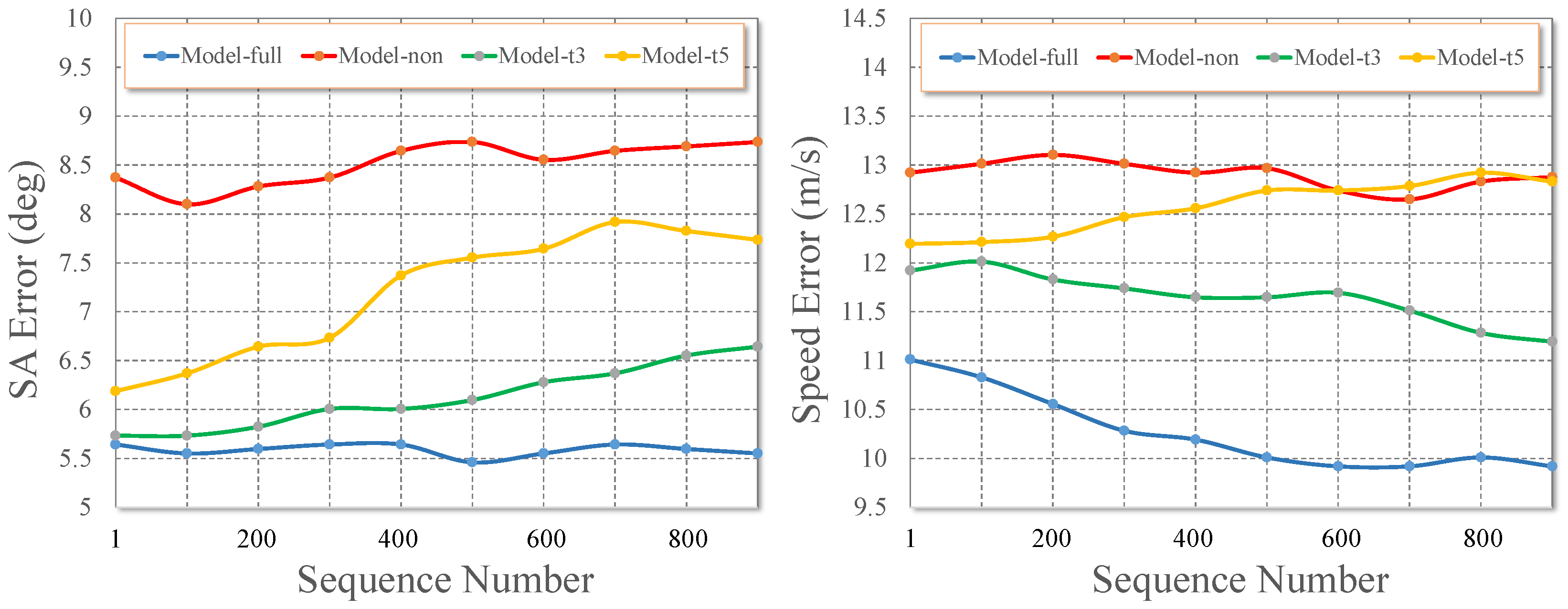
5.1. Accuracy Evaluation on Benchmarks

We firstly provide the driving accuracy comparison, including the steering angle (SA) and speed value (SPD) with some state-of-the-art approaches based on two benchmarks so as to evaluate the performance of reliability quantitatively. Specifically, we use MAE (Mean Absolute Error) to evaluate the error between the ground truth and the predicted control commands, as shown below.

$$\begin{array}{c}\hfill MAE={\displaystyle \frac{1}{N-2}}\sum _{t=2}^{N-1}\left|\left(\widehat{x_t}-x_t\right)\right|,\end{array}$$

(7)

where $x_t\in {\mathbb{R}}^{1\times 1}$ represents the estimated steering angle or speed value at time $\mathit{t}$, and $\widehat{x_t}$ is the corresponding ground truth. $\mathit{N}$ is the number of images in a sequence. We start counting the sample numbers from the second image since the first FDI is created by using [${\mathit{I}}_1$, ${\mathit{I}}_2$].

We analyze the performance of reliability on PilotNet [6], Cg Network (https://github.com/udacity/self-driving-car/tree/master/steering-models/community-models/cg23, accessed on 1 April 2025), PCNN [25], DeepVO [7], and our autonomous driving model. At this step, we only use the current control commands [$s_t$,$v_t$] in comparison since the upcoming control commands [${\mathit{s}}_{\mathit{t}+1}$,${\mathit{v}}_{\mathit{t}+1}$] are in charge of improving efficiency. Note that we use a modified version of DeepVO and a modified version of PCNN in the comparison in which their output nodes are set to 2 in order to predict the steering angle and the speed value simultaneously.

The results are summarized in

Table 2. Comparison of the steering angle and the speed value by use of Mean Absolute Error (MAE).

Seq.	Our Model		DeepVO		PCNN		PilotNet		Cg Network
	SA (deg)	SPD (m/s)	SA (deg)	SPD (m/s)	SA (deg)	SPD (m/s)	SA (deg)	SPD (m/s)	SA (deg)	SPD (m/s)
KITTI/City/2011-09-26-drive-0009	7.89	9.86	7.72	10.99	7.68	11.69	12.57	13.85	17.64	21.74
KITTI/Residential/2011-09-26-drive-0019	4.60	7.39	7.35	11.50	8.76	17.18	14.54	17.48	19.16	26.55
KITTI/Road/2011-09-26-drive-0028	6.72	8.95	8.84	12.39	7.44	15.12	16.97	19.45	20.84	21.29
RobotCar/2014-06-25-16-22-15-sun	5.79	7.20	5.52	9.59	5.83	12.49	12.51	16.28	15.24	19.08
RobotCar/2014-12-05-11-09-10-rain	4.32	7.75	6.19	13.14	7.08	14.75	15.43	17.75	21.07	26.22
RobotCar/2015-02-03-08-45-10-snow	3.36	5.78	7.46	12.35	8.16	17.06	14.35	21.96	13.15	18.94
RobotCar/2015-02-03-19-43-11-night	6.12	10.80	12.68	18.41	17.52	22.75	12.89	27.59	23.28	28.67
Average	5.54	8.25	7.97	12.62	8.92	15.86	14.18	19.19	18.63	23.21

$SA$ ($\mathrm{deg}$) average error of the steering angle under different road conditions and scenes. $SPD$ ($\mathrm{m}/\mathrm{s}$) average error of the speed value under different road conditions and scenes.

. First, we observe that DeepVO and our autonomous driving model obtain closer MAEs in the prediction of the steering angle, and DeepVO has a relatively large MAE in the prediction of the speed value. We believe that DeepVO learns the long-term dependencies directly from raw images, which have limited ability to sense the motion change between nearby frames. In some test sequences, e.g., KITTI/city and RobotCar/sun, the steering angle prediction of DeepVO and PCNN has a slight advantage over ours, since these sequences contain mostly clear lanes and better weather conditions. Our method obtains more satisfactory results than DeepVO when testing under relatively complex road conditions, i.e., KITTI/Residential and KITTI/Road, and different weather, e.g., RobotCar/rain and RobotCar/snow, since FDIs are able to reveal the most critical changes between frame pairs and such difference images are not sensitive to environmental changes. In sequences of RobotCar/night, the performance of DeepVO dramatically drops when compared with ours (${6.12}^{\circ }$ and $10.8$ m/s vs. ${12.68}^{\circ }$ and $18.41$ m/s) since we did not use a similar dataset to train the above models, and this proves the generalization ability of our model. PCNN takes dense optic flow as input to predict the driving controls, in which its steering prediction is relatively higher since the optic flow contains the information of motion changes. Nevertheless, the predicted speed values have relatively larger MAE due to the network being constructed via the combination of CNNs and fully connected layers. Hence, there is a lack of ability to learn from consecutive sequences. PilotNet and Cg Network have relatively low accuracy in steering angle and speed value prediction since these models have no RNN layers to learn long-term dependencies. The predictions of the above two networks have relatively larger fluctuations, which may lead to a zigzag steering control during driving.

In the KITTI dataset, FDI activates only approximately 1.8–22.3% of inter-frame pixels, which correspond to motion boundaries and geometrically discontinuous structures (e.g., road marking discontinuities, vehicle contours). This sparse activation pattern closely aligns with human visual attention mechanisms, thereby compelling the model to abandon redundant static texture processing. By concentrating computational resources on parsing critical geometric structures, the model significantly enhances its accuracy in predicting driving behaviors. Hence, the predicted steering angle achieves an average MAE of $5.{54}^{\circ }$ and an average speed of $8.25$ m/s on seven different sequences. In addition to the current control commands, we also determine the accuracy of the upcoming control commands, and we found that the difference between these two predictions is much closer. Specifically, compared with the current control commands, the upcoming one with approximately $0.79\%$ in the steering angle error and $1.1\%$ in the speed value error. Our autonomous driving model supports the accurate and reliable driving actions under different road and weather conditions.

We randomly select 900 images (400 in KITTI and 500 in RobotCar) as samples from the testing sets illustrated in Table 2. Then, we conduct the ablation with a series of modified versions of our autonomous driving models.

As shown in Figure 5, for the prediction of upcoming driving actions, we set up three modified versions of our proposed model, which are Model-non, Model-t3 and Model-t5. Model-full is the original version of our proposed model. Model-non is not initialized and fixed with pre-trained weights on the $\mathit{CNN}2$ structure. For Model-t3 and Model-t5, we predict the upcoming control commands for $t+3$ and $t+5$, respectively Comparing Model-full and Model-non, we found that the errors of both steering angle and speed are significantly increased (approx. $5.5^{\circ }$ to $8.5^{\circ }$ for SA Error; $10.4$ m/s to $12.9$ m/s for Speed Error). This gives a clear insight that the module of the upcoming-view synthesis is able to generate the accurate extra control commands for the future. The comparison results of Model-t3 and Model-t5 demonstrate that our model has a generalization ability to predict the driving actions for the relatively further future. As the time interval increases, the accuracy of the prediction drops. Especially for the speed prediction on Model-t5, the performance is close to Model-non. We believe that the reason is the driving behaviors, in which the vehicle speed is changed frequently when the time interval is longer than a second. Our Model-full keeps relatively better performance since it predicts driving actions for $t+1$ and the time interval is close to the frame rate (10 Hz) of the cameras. In our experience, driving speed hardly changes during this time interval.

For the prediction of current driving actions, we set up four modified versions of the proposed model, which are Model-raw, Model-FDI, Model-full (t3) and Model-full (t5), as shown in Figure 6, Note that Model-full (t3) and Model-full (t5) calculate the FDI by using images at $t+3$ and $t+5$, respectively. The results in Figure 6 indicate that the error of steering angle and speed is increasing by using only raw images as input to predict the driving actions. We believe that raw images contain redundant information which will bring abundant uncertainty to the system. Additionally, the system may need a much deeper convolutional structure, e.g., VGG-16, to encode the temporal information from raw images. This will increase the computational complexity for the system to some degree. Model-FDI and Model-full have similar performance, and this implies that we should make a balance between the textural input and the temporal information so as to achieve accurate and reliable predictions. In addition, Model-full (t3) and Model-full (t5) lose accuracy as the time interval increases. It has a relatively significant influence on speed prediction since sequences in benchmarks are collected under slow speed.

5.2. Evaluation of Energy-Efficiency

In this experiment, a P3-AT mobile robot, as shown in Figure 7a, is deployed in the outside environment to evaluate different autonomous driving models and energy-efficiency policies. To achieve this, we add a power analyzer in series between the batteries and the robot’s power distribution board. This allows us to evaluate energy efficiency during robot movement in terms of the instantaneous power consumption.

Experiments were conducted on three paths, i.e., Path 01 (approx. 125 m, with curves), Path 02 (approx. 105 m, with pedestrians) and Path 03 (approx. 110 m, during daytime and nighttime) in the outdoor environment, as shown in Figure 7b–d. We evaluate energy efficiency by using three different control policies, i.e., Policy-v1, Policy-v2 and Policy-v3. More specifically, Policy-v1 achieves driving efficiency through Equation (6). Policy-v2 uses the historical control command [${\mathit{s}}_{\mathit{t}-1}$,${\mathit{v}}_{\mathit{t}-1}$] and the current one [$s_t$,$v_t$] as input. Policy-v3 keeps a constant driving speed when the system is running, and only steering angle smoothing is applied (by using Policy-v2). Additionally, we compare the instantaneous power consumption with other approaches. Note that, since the approaches (PilotNet and Cg Network) have unsatisfactory performance in the evaluation of reliability, here we only add DeepVO to the experiment. Here, DeepVO uses Policy-v2 to smooth driving actions. As mentioned in Section 4.4, $\lambda$ in Equation (6) is set to $0.65$ empirically. The result in

Table 3. Average value of instantaneous power consumption (unit: milliwatt) under three paths in outdoor environments.

Seq.	Policy-v1	Policy-v2	Policy-v3	DeepVO
Path 01	12,593.43	13,584.53	13,511.37	13,409.21
Path 02	8576.61	9712.62	8945.49	10,246.49
Path 03 (daytime)	6174.95	6651.74	6784.08	6718.05
Path 03 (nighttime)	6645.28	7059.08	6916.15	7162.57
Average	8497.57	9251.99	9039.27	9384.08

Note that three versions of control policies (v1–v3) for our method, plus one approach (DeepVO), are compared in the evaluation.

demonstrates that Policy-v1 achieves the most efficient driving control among the three driving policies. Policy-v2 and Policy-v3 are relatively costly in terms of energy consumption when compared to Policy-v1. These two policies consume extra power in the amount of approximately 1.09% and 1.06% (in the average value), respectively. The result demonstrates that the historical control command only has the ability to achieve smoothness. However, it has limited ability to guide the vehicle driving efficiently. Additionally, we found that DeepVO and ours (Policy-v2) have similar performance when testing on $\mathit{Path}01$. Disturbed by pedestrians, such as $\mathit{Path}02$, the performance of DeepVO drops 1.19%. The difference between DeepVO and ours (Policy-v2) on $\mathit{Path}03$ during daytime is approximately 1.09%, and the situation becomes worse when testing on $\mathit{Path}03$ during nighttime. The robot deviates from the straight direction halfway through and hits the edge of the road, as shown in Figure 7d, and hence we only use the data before the collision to perform the evaluation (DeepVO drops approx. 1.08%). By contrast, our autonomous driving method uses the upcoming controls, which achieves, through the extra information of the upcoming-view synthesis module, the creation of the driving policy. The upcoming view allows the vehicle to foreknow the view in the future based on the historical information. It may have the ability to avoid unexpected driving actions, e.g., sudden braking or turning, to some degree.

We set up the experiment by using the robot in daytime on $\mathit{Path}03$ in order to measure the performance change under three smoothness strategies. The result in Figure 8 illustrates that the power consumption will increase dramatically (approx. 47.6%) without the use of any strategies for smoothness.

By smoothing the steering controls, the robot saves a large amount of electrical energy, and the smoothness of the speed controls can save energy further. The reason is that P3-AT adopts a differential motion structure while moving, and it will cause significant current changes when steering. The robot needs relatively lower current under the state of uniform linear motion.

5.3. Efficiency of Driving Behavior

To our knowledge, driving behavior has not been fully considered in recent research. Hence, we performed exploratory research in this aspect and illustrated a part of the results in this section. In our manuscript, we discussed energy-efficient vehicle control based on different policies of driving smoothness, e.g., Policy-v1, Policy-v2, and Policy-v3. However, recent benchmarks for autonomous driving are crowd-sourced data collected from different drivers who may have different driving experiences. Driving behavior is a complex variable that may lead to unsatisfactory performance for end-to-end driving models. In our opinion, energy-efficient vehicle control is not only dominated by smoothness policies but also influenced by the quality of data collection. For instance, if the model is trained with sequences which contain mostly inefficient driving controls, it may result in an unsatisfactory driving experience, even though the prediction comes with high accuracy. On the one hand, the recent crowd-sourcing data is mixed with different driving behaviors of drivers, and some redundant control methods are included unavoidably. On the other hand, the general benchmarks record insufficient driving behavior for the same path. For example, the KITTI benchmark contains mostly one-way trips. The Oxford RobotCar benchmark contains repeated paths with different situations, e.g., weather, brightness, and road conditions. Our goal is to explore how the performance may change by using different driving behaviors. Hence, we use the Udacity self-driving car simulator to collect datasets which contain distinct driving behaviors, as shown in Figure 9a. Then, we use a different portion of the datasets to train our autonomous driving model so as to evaluate the influence relating to different driving behaviors.

In our experiment, we invited 10 volunteers to join the simulated driving under two different virtual scenes, i.e., Scene 01 and Scene 02, in order to record their control commands which imply unique control behavior. For each scene, each volunteer plays a round trip three times, so we collect 60 samples in total. We encourage people to drive the virtual car with efficiency and safety, in which unnecessary operations and failure cases can be avoided as much as possible. However, even under this requirement, people will make distinct decisions during driving according to their experiences, as shown in Figure 9b. To solve the above problem, we define five landmarks in $\mathit{Scene}01$ and nine landmarks in $\mathit{Scene}02$, and then we segment the whole path into several segments according to the same landmarks. Each segment contains different driving commands and we manually align these driving commands together in order to draw the driving command changes using the method of the box-plot. The box-plot contains the upper and lower bounds (UB and LB), the upper and lower quartiles (UQ and LQ), and a median value (MV). Note that we only plot the steering angle change here, since the velocity value has a slight change in most parts of the scenes. From observation, we found that the driving controls obey a statistical distribution. For instance, the most efficient control commands appear frequently and appear near the MV. The inefficient control commands, which may be caused by misjudgment or redundant operations, are distributed in the range of UB and LB.

The result in Figure 10 demonstrates that the model trained with the control commands in range of the UQ and LQ shows efficiency during the test. The predicted control commands are close to the MV and mostly distributed in the range of the UQ and LQ. The model that trained with the whole dataset reports relatively weak performance of driving smoothness since the steering predictions have a larger fluctuation when compared with the median value. Results on the simulator illustrate that diverse behaviors can affect driving efficiency, especially for the data which are acquired in the crowd-sourced manner. If we want to improve the driving efficiency further, the quality of the driving data should be considered.

6. Conclusions and Future Works

In this paper, we propose a robust and energy-efficient autonomous driving method. Benefiting from two auxiliary tasks, our method can perform smooth driving actions under different road conditions, and it shows robustness when encountering the changes in weather or time. The main problem of the learning-based autonomous driving approaches is that the performance of driving highly depends on the drivers, especially for the crowd-sourced data. We already conducted some research based on the Udacity self-driving simulator in order to explore the relationship between driving behavior and driving efficiency. Since this study employs an end-to-end model for driving behavior prediction, the optical flow or depth map predictions are implicitly represented within the model. Due to the scope of this study, the evaluation of optical flow or depth map predictions and the analysis of their impact on the final control commands are not included in the current evaluation. We will conduct dedicated research and experiments on this issue in future work. Additionally, we will consider integrating extra applications to enhance the ability of scene and object recognition, such as the works in [43,44]. Combining our autonomous driving method with a navigation component, as in [45,46], would greatly improve the practicability under a real road environment and unleash the advantages of end-to-end learning paradigms. These ideas will drive our research in the future.

References

1. Wang, B.; Bessaad, N.; Xu, H.; Zhu, X.; Li, H. Mergeable Probabilistic Voxel Mapping for LiDAR–Inertial–Visual Odometry. Electronics 2025, 14, 2142. [Google Scholar] [CrossRef]
2. Zhang, T.; Xia, Z.; Li, M.; Zheng, L. DIN-SLAM: Neural Radiance Field-Based SLAM with Depth Gradient and Sparse Optical Flow for Dynamic Interference Resistance. Electronics 2025, 14, 1632. [Google Scholar] [CrossRef]
3. Zhang, Y.; Shi, P.; Li, J. 3d lidar slam: A survey. Photogramm. Rec. 2024, 39, 457–517. [Google Scholar] [CrossRef]
4. Kato, S.; Takeuchi, E.; Ishiguro, Y.; Ninomiya, Y.; Takeda, K.; Hamada, T. An open approach to autonomous vehicles. IEEE Micro 2015, 35, 60–68. [Google Scholar] [CrossRef]
5. Zhu, F.; Ma, L.; Xu, X.; Guo, D.; Cui, X.; Kong, Q. Baidu apollo auto-calibration system-an industry-level data-driven and learning based vehicle longitude dynamic calibrating algorithm. arXiv 2018, arXiv:1808.10134. [Google Scholar]
6. Bojarski, M.; Testa, D.D.; Dworakowski, D.; Firner, B.; Flepp, B.; Goyal, P.; Jackel, L.D.; Monfort, M.; Muller, U.A.; Zhang, J.; et al. End to End Learning for Self-Driving Cars. arXiv 2016, arXiv:1604.07316. [Google Scholar] [CrossRef]
7. Wang, S.; Clark, R.; Wen, H.; Trigoni, N. DeepVO: Towards end-to-end visual odometry with deep Recurrent Convolutional Neural Networks. In Proceedings of the International Conference on Robotics and Automation, Shanghai, China, 29–31 December 2017; pp. 2043–2050. [Google Scholar]
8. Wang, S.; Clark, R.; Wen, H.; Trigoni, N. End-to-end, sequence-to-sequence probabilistic visual odometry through deep neural networks. Int. J. Robot. Res. 2018, 37, 513–542. [Google Scholar] [CrossRef]
9. Xu, H.; Gao, Y.; Yu, F.; Darrell, T. End-to-End Learning of Driving Models from Large-Scale Video Datasets. In Proceedings of the Computer Vision and Pattern Recognition, Honolulu, HI, USA, 21–26 July 2017; pp. 3530–3538. [Google Scholar]
10. Huval, B.; Wang, T.; Tandon, S.; Kiske, J.; Song, W.; Pazhayampallil, J.; Andriluka, M.; Rajpurkar, P.; Migimatsu, T.; Chengyue, R.; et al. An Empirical Evaluation of Deep Learning on Highway Driving. arXiv 2015, arXiv:1504.01716. [Google Scholar] [CrossRef]
11. Chen, X.; Kundu, K.; Zhang, Z.; Ma, H.; Fidler, S.; Urtasun, R. Monocular 3D Object Detection for Autonomous Driving. In Proceedings of the Computer Vision and Pattern Recognition, Las Vegas, NV, USA, 27–30 June 2016; pp. 2147–2156. [Google Scholar]
12. Chen, C.; Seff, A.; Kornhauser, A.; Xiao, J. DeepDriving: Learning Affordance for Direct Perception in Autonomous Driving. In Proceedings of the The IEEE International Conference on Computer Vision (ICCV), Santiago, Chile, 7–13 December 2015; pp. 2722–2730. [Google Scholar]
13. Posch, C.; Serrano-Gotarredona, T.; Linares-Barranco, B.; Delbruck, T. Retinomorphic Event-Based Vision Sensors: Bioinspired Cameras With Spiking Output. Proc. IEEE 2014, 102, 1470–1484. [Google Scholar] [CrossRef]
14. Mueggler, E.; Rebecq, H.; Gallego, G.; Delbruck, T.; Scaramuzza, D. The Event-Camera Dataset and Simulator: Event-based Data for Pose Estimation, Visual Odometry, and SLAM. Int. J. Robot. Res. 2017, 36, 142–149. [Google Scholar] [CrossRef]
15. Ghosh, R.; Mishra, A.; Orchard, G.; Thakor, N.V. Real-time object recognition and orientation estimation using an event-based camera and CNN. In Proceedings of the IEEE 2014 Biomedical Circuits and Systems Conference, BioCAS 2014, Lausanne, Switzerland, 22–24 October 2014; pp. 544–547. [Google Scholar]
16. Maqueda, A.I.; Loquercio, A.; Gallego, G.; Garcla, N.; Scaramuzza, D. Event-Based Vision Meets Deep Learning on Steering Prediction for Self-Driving Cars. In Proceedings of the The IEEE Conference on Computer Vision and Pattern Recognition (CVPR), Salt Lake City, UT, USA, 18–23 June 2018; pp. 5419–5427. [Google Scholar]
17. Lotter, W.; Kreiman, G.; Cox, D.D. Deep Predictive Coding Networks for Video Prediction and Unsupervised Learning. arXiv 2016, arXiv:1605.08104. [Google Scholar]
18. Tatarchenko, M.; Dosovitskiy, A.; Brox, T. Single-view to Multi-view: Reconstructing Unseen Views with a Convolutional Network. arXiv 2015, arXiv:1511.06702. [Google Scholar]
19. Zhou, T.; Tulsiani, S.; Sun, W.; Malik, J.; Efros, A.A. View Synthesis by Appearance Flow. In Proceedings of the European Conference on Computer Vision (2016), Amsterdam, The Netherlands, 11–14 October 2016; pp. 286–301. [Google Scholar]
20. Baras, N.; Nantzios, G.; Ziouzios, D.; Dasygenis, M. Autonomous Obstacle Avoidance Vehicle Using LIDAR and an Embedded System. In Proceedings of the 2019 8th International Conference on Modern Circuits and Systems Technologies (MOCAST), Thessaloniki, Greece, 13–15 May 2019; pp. 1–4. [Google Scholar] [CrossRef]
21. Li, Y.; Ma, L.; Zhong, Z.; Liu, F.; Chapman, M.A.; Cao, D.; Li, J. Deep Learning for LiDAR Point Clouds in Autonomous Driving: A Review. IEEE Trans. Neural Netw. Learn. Syst. 2020, 32, 3412–3432. [Google Scholar] [CrossRef] [PubMed]
22. Hane, C.; Heng, L.; Lee, G.H.; Fraundorfer, F.; Furgale, P.; Sattler, T.; Pollefeys, M. 3D visual perception for self-driving cars using a multi-camera system: Calibration, mapping, localization, and obstacle detection. Image Vis. Comput. 2017, 68, 14–27. [Google Scholar] [CrossRef]
23. Mathew, A.; Mathew, J. Monocular depth estimation with SPN loss. Image Vis. Comput. 2020, 100, 103934. [Google Scholar] [CrossRef]
24. Chen, J.; Bai, T. SAANet: Spatial adaptive alignment network for object detection in automatic driving. Image Vis. Comput. 2020, 94, 103873. [Google Scholar] [CrossRef]
25. Costante, G.; Mancini, M.; Valigi, P.; Ciarfuglia, T.A. Exploring Representation Learning With CNNs for Frame-to-Frame Ego-Motion Estimation. IEEE Robot. Autom. Lett. 2016, 1, 18–25. [Google Scholar] [CrossRef]
26. Amini, A.; Gilitschenski, I.; Phillips, J.; Moseyko, J.; Banerjee, R.; Karaman, S.; Rus, D. Learning Robust Control Policies for End-to-End Autonomous Driving From Data-Driven Simulation. IEEE Robot. Autom. Lett. 2020, 5, 1143–1150. [Google Scholar] [CrossRef]
27. Kim, J.; Canny, J. Interpretable learning for self-driving cars by visualizing causal attention. In Proceedings of the The IEEE International Conference on Computer Vision (ICCV), Venice, Italy, 22–29 October 2017; pp. 2942–2950. [Google Scholar]
28. Hyndman, R.; Koehler, A.B.; Ord, J.K.; Snyder, R.D. Forecasting with Exponential Smoothing: The State Space Approach; Springer Science and Business Media: Berlin/Heidelberg, Germany, 2008. [Google Scholar]
29. Yang, Z.; Zhang, Y.; Yu, J.; Cai, J.; Luo, J. End-to-end multi-modal multi-task vehicle control for self-driving cars with visual perception. In Proceedings of the International Conference on Pattern Recognition (ICPR), Beijing, China, 10–24 August 2018. [Google Scholar]
30. Rebecq, H.; Gehrig, D.; Scaramuzza, D. In Proceedings of the ESIM: An Open Event Camera Simulator, Zürich, Switzerland, 29–31 October 2018.
31. Yang, J.; Zhao, Y.; Jiang, B.; Lu, W.; Gao, X. No-Reference Quality Evaluation of Stereoscopic Video Based on Spatio-Temporal Texture. IEEE Trans. Multimed. 2019, 22, 2635–2644. [Google Scholar] [CrossRef]
32. Li, Z.; Hu, H.; Zhang, W.; Pu, S.; Li, B. Spectrum Characteristics Preserved Visible and Near-Infrared Image Fusion Algorithm. IEEE Trans. Multimed. 2020, 23, 306–319. [Google Scholar] [CrossRef]
33. Shepard, R.N.; Metzler, J. Mental Rotation of Three-Dimensional Objects. Science 1971, 171, 701–703. [Google Scholar] [CrossRef] [PubMed]
34. Li, K.; Wu, Y.; Xue, Y.; Qian, X. Viewpoint Recommendation Based on Object Oriented 3D Scene Reconstruction. IEEE Trans. Multimed. 2020, 23, 257–267. [Google Scholar] [CrossRef]
35. Li, L.; Zhou, Y.; Wu, J.; Li, F.; Shi, G. Quality Index for View Synthesis by Measuring Instance Degradation and Global Appearance. IEEE Trans. Multimed. 2020, 23, 320–332. [Google Scholar] [CrossRef]
36. Rosin, P.; Ellis, T. Image difference threshold strategies and shadow detection. In Proceedings of the British Machine Vision Conference, Birmingham, UK, 11–14 September 1995. [Google Scholar]
37. Geiger, A.; Lenz, P.; Urtasun, R. Are we ready for autonomous driving? the kitti vision benchmark suite. In Proceedings of the Conference on Computer Vision and Pattern Recognition (CVPR), Providence, RI, USA, 16–21 June 2012. [Google Scholar]
38. Maddern, W.; Pascoe, G.; Linegar, C.; Newman, P. 1 Year, 1000 km: The Oxford RobotCar Dataset. Int. J. Robot. Res. (IJRR) 2017, 36, 3–15. [Google Scholar] [CrossRef]
39. Simonyan, K.; Zisserman, A. Very deep convolutional networks for large-scale image recognition. arXiv 2014, arXiv:1409.1556. [Google Scholar]
40. Kreuzig, R.; Ochs, M.; Mester, R. DistanceNet: Estimating Traveled Distance From Monocular Images Using a Recurrent Convolutional Neural Network. In Proceedings of the IEEE/CVF Conference on Computer Vision and Pattern Recognition Workshops, Long Beach, CA, USA, 16–17 June 2019; pp. 69–77. [Google Scholar]
41. Lefevre, S.; Carvalho, A.; Borrelli, F. A Learning-Based Framework for Velocity Control in Autonomous Driving. IEEE Trans. Autom. Sci. Eng. 2016, 13, 32–42. [Google Scholar] [CrossRef]
42. Geiger, A.; Lenz, P.; Stiller, C.; Urtasun, R. Vision meets robotics: The kitti dataset. Int. J. Robot. Res. 2013, 32, 1231–1237. [Google Scholar] [CrossRef]
43. Pei, Y.; Sun, B.; Li, S. Multifeature Selective Fusion Network for Real-Time Driving Scene Parsing. IEEE Trans. Instrum. Meas. 2021, 70, 5008412. [Google Scholar] [CrossRef]
44. Hu, H.; Zhao, T.; Wang, Q.; Gao, F.; He, L.; Gao, Z. Monocular 3-D Vehicle Detection Using a Cascade Network for Autonomous Driving. IEEE Trans. Instrum. Meas. 2021, 70, 5012213. [Google Scholar] [CrossRef]
45. Seff, A.; Xiao, J. Learning from Maps: Visual Common Sense for Autonomous Driving. arXiv 2016, arXiv:1611.08583. [Google Scholar] [CrossRef]
46. Yan, Z.; Zhang, C.; Yang, Y.; Liang, J. A Novel In-Motion Alignment Method Based on Trajectory Matching for Autonomous Vehicles. IEEE Trans. Veh. Technol. 2021, 70, 2231–2238. [Google Scholar] [CrossRef]
Figure 1. Our autonomous driving model takes frame-to-frame difference images (FDIs) as input, in which FDIs can eliminate image redundancy and reveal the most important features from raw sequences. This allows us to guarantee the reliability of vehicle controls in complex environments.
Electronics 14 02919 g001
Figure 2. The overview of our proposed method, in which the autonomous driving model (C) takes two components as auxiliary tasks (A,B) to implement reliability and driving efficiency.
Electronics 14 02919 g002
Figure 3. Visual comparison between raw images and FDIs in typical scenes. On the one side, FDIs are able to highlight the change in driving states, such as high (a) or low (b) driving speed, state of turning a corner (c), or stopping (d). On the other side, FDIs are less affected by illumination variation, i.e., (eg), and weather changes (h).
Electronics 14 02919 g003
Figure 4. Visual comparison between raw images and synthetic upcoming views. The synthetic images can recover the road surfaces (a,b), buildings (c), and traffic (d). The views can be recovered when facing a quick turn, as in (e,f). Additionally, vehicles with different moving directions can be predicted precisely, as in (g,h). The synthetic upcoming views can be used to assist the autonomous vehicles to sense the road conditions for the next moment.
Electronics 14 02919 g004
Figure 5. The error of the upcoming steering angles (SAs) by using different versions of our model when compared to the ground truth.
Electronics 14 02919 g005
Figure 6. The error of the current steering angles (SAs) with the use of different inputs when compared to the ground truth.
Electronics 14 02919 g006
Figure 7. A mobile robot (a) is deployed on three paths (bd) to implement different policies of driving controls so as to collect the power consumption for analysis. The complexity of the real world may lead the robot to distinct trajectories and even a collision (e).
Electronics 14 02919 g007
Figure 8. The instantaneous power of the mobile robot by using different strategies of smoothness controls or energy-efficient policies.
Electronics 14 02919 g008
Figure 9. We use the simulator (a) to collect driving behavior from volunteers, in which each person has their unique control strategy (b) under the same road conditions.
Electronics 14 02919 g009
Figure 10. Result of the driving model trained by using different portions of the collected data.
Electronics 14 02919 g010