Deep Edge IoT for Acoustic Detection of Queenless Beehives

Abstract

Honey bees play a vital role in ecosystem stability, and the need to monitor colony health has driven the development of IoT-based systems in beekeeping, with recent studies exploring both empirical and machine learning approaches to detect and analyze key hive conditions. In this study, we present an IoT-based system that leverages sensors to record and analyze the acoustic signals produced within a beehive. The captured audio data is transmitted to the cloud, where it is converted into mel-spectrogram representations for analysis. We explore multiple data pre-processing strategies and machine learning (ML) models, assessing their effectiveness in classifying queenless states. To evaluate model generalization, we apply transfer learning (TL) techniques across datasets collected from different hives. Additionally, we implement the feature extraction process and deploy the pre-trained ML model on a deep edge IoT device (Arduino Zero). We examine both memory consumption and execution time. The results indicate that the selected feature extraction method and ML model, which were identified through extensive experimentation, are sufficiently lightweight to operate within the device’s memory constraints. Furthermore, the execution time confirms the feasibility of real-time queenless state detection in edge-based applications.

1. Introduction

Pollination plays a crucial role in fertilization and seed production, directly impacting the well-being of ecosystems globally. Among the various pollinators, the honey bee (Apis mellifera) is a significant contributor, estimated to be responsible for over 90% of global commercial pollination services and approximately 35% of the world’s food crops [1]. In addition to pollination, honey bees produce important and delicate substances such as honey, beeswax, propolis, and royal jelly [2], which are widely utilized by humans for various purposes. However, honey bee populations face numerous threats, including parasites, ants, hive beetles, and hive robberies, which can lead to colony collapse [3].

Honeybees produce rhythmic thoracic oscillations transmitted as substrate vibrations or airborne sounds to communicate within the hive [4]. These vibroacoustic signals influence behaviors related to swarming, including the queen’s actions [5]. The colony’s “sound,” a continuous low-frequency buzz, results from individual bee signals, with frequencies primarily around 300, 410, and 500 Hz but surely within the range of 100 to 1000 Hz [6]. The absence of a queen results in the production of a “warble” signal, characterized by a frequency of 225–285 Hz during the first 5 h. Subsequently, the signal transitions into a roaring sound with a frequency of 180 Hz [7]. Both the frequency range and signal pattern are crucial for detecting potential threats to the colony [8]. Previous studies have used methods such as endoscopic observations, calorimetric traces, accelerometer recordings, and electric field measurements [9,10,11]. Sound data was typically pre-processed with a band-pass filter (high-frequency cut-off at 2 kHz, low-frequency cut-offs between 20 and 100 Hz) [12,13]. Additional techniques like wavelet decomposition, spectral subtraction, Mel Frequency Cepstral Coefficients (MFCCs) [14], Hilbert Huang Transform (HHT) with wavelet analysis, Linear Predictive Coding (LPC) [13], and Short-Time Fourier Transform (STFT) [15] have also been used for feature extraction and analysis.

Several studies [16,17,18,19,20,21,22,23] have proposed the integration of IoT technologies and sensors to automate various aspects of beekeeping. In particular, the work presented in [16] introduces a multi-sensor system designed to measure key metrics such as hive weight, acoustic signals, internal and external temperature, relative humidity, and ${\mathrm{CO}}_2$ levels under normal conditions. Additionally, the system aims to analyze these parameters during specific phenomena, such as honey gathering and swarming, to establish correlations between these events and the recorded sensor data. In [17], a multi-sensor system is proposed to measure weather-related parameters both inside and outside the hive, along with a bee counter positioned at the hive entrance. Furthermore, studies in [18,22] introduce an imaging system at the hive entrance to monitor honey bee activity. Similarly, the works presented in [20,21] propose IoT-based systems designed to collect data and transmit it to the cloud for analysis, specifically for detecting Varroa infestation, a parasitic infection affecting honey bees. Additionally, the study in [23] proposes a multi-sensor system to collect vocal, image, and weather data, while also publicly releasing their collected datasets.

One important factor that can be monitored electronically is the presence or absence of a queen within the hive [24]. The absence of a queen within a hive is a key indicator of health concerns and may signal impending colony failure, as the queen is essential to the overall health of the hive. Several approaches have been proposed to detect the absence of a queen within a hive. Uthoff et al. [7] provide a comprehensive review of such methods, highlighting various studies that utilize weather-related data, acoustic signals, and other hive parameters. These approaches, often integrated with Machine Learning (ML) and Deep Learning (DL) techniques, have demonstrated effectiveness in identifying queenless states and swarming events.

In [24], an Internet-of-Things (IoT) system utilizing a low-power microcontroller (MCU) is introduced to detect the presence of a queen bee based on audio recordings from the hive. The system employs a Tiny Machine Learning (TinyML) classifier, aiming for high-accuracy predictions while maintaining low power consumption, making it suitable for resource-constrained edge devices. The study explores Neural Networks (NNs) and Support Vector Machines (SVMs), with a primary focus on NNs due to the lack of quantization methods for SVMs in conventional libraries. Similarly, in Ref. [25], various Machine Learning (ML) models, including K-Nearest Neighbors (KNN), Multilayer Perceptron (MLP), Random Forest (RF), and Support Vector Machine (SVM), were evaluated to classify hives as queenright or queenless. The study utilized two types of data: microclimatic and bioacoustic. Notably, data for the queenless state was collected from already queenless hives, ensuring accurate representation of this condition. On the other hand, Refs. [26,27] proposed the use of Convolutional Neural Networks (CNNs) to characterize and classify hives as queenless or queenright based on acoustic recordings. This approach involved a sound processing procedure to extract relevant features before classification, leveraging CNNs’ ability to analyze complex acoustic patterns. Additionally, in Refs. [28,29], various models, including classical Machine Learning (ML) techniques and Convolutional Neural Networks (CNNs), were examined and evaluated for classifying hives as queenless or queenright. These studies aimed to assess the effectiveness of different approaches in accurately detecting the queen’s presence based on hive data. Finally, some studies have explored the use of Long Short-Term Memory (LSTM) networks for monitoring the queenless state of a hive [29,30]. These approaches leverage LSTMs’ ability to capture temporal dependencies in acoustic or environmental data, enhancing the accuracy of queen state classification.

In this study, we present an IoT-based system that utilizes sensors to capture and analyze the acoustic signals produced by a beehive. The collected data is transmitted to the cloud for processing, where it is transformed, adopting Mel Frequency Cepstral Coefficients (MFCCs) into mel-spectrogram representations, and used as input for machine learning (ML) models trained to detect the queenright/queenless state of a hive. We evaluate multiple ML models based on their classification performance for queenright/queenless state classification. Additionally, we assess their ability to generalize to unseen data by employing transfer learning (TL) techniques across models trained on different hives. In the final stage, the feature extraction process and the inference of the pre-trained machine learning model are deployed on a deep edge IoT platform (Arduino Zero). A comprehensive evaluation of memory usage and execution time is conducted. The findings indicate that the chosen feature extraction technique and machine learning model, selected through rigorous experimentation, are adequately lightweight to operate within the memory limitations of the device. Additionally, the execution time meets the requirements for real-time performance in edge-based queenless hive detection scenarios.

2. Materials and Methods

This section provides a description of the experimental process followed to create the dataset and the step-by-step methodology for the classification between the presence or the absence of the queen bee based on sound recordings. This includes all the information regarding the dataset, the pre-processing and the extraction of the MFFC features, as well as the methodology for determining the feature importance, the approach for training, testing, evaluating, and implementation of the ML models under investigation.

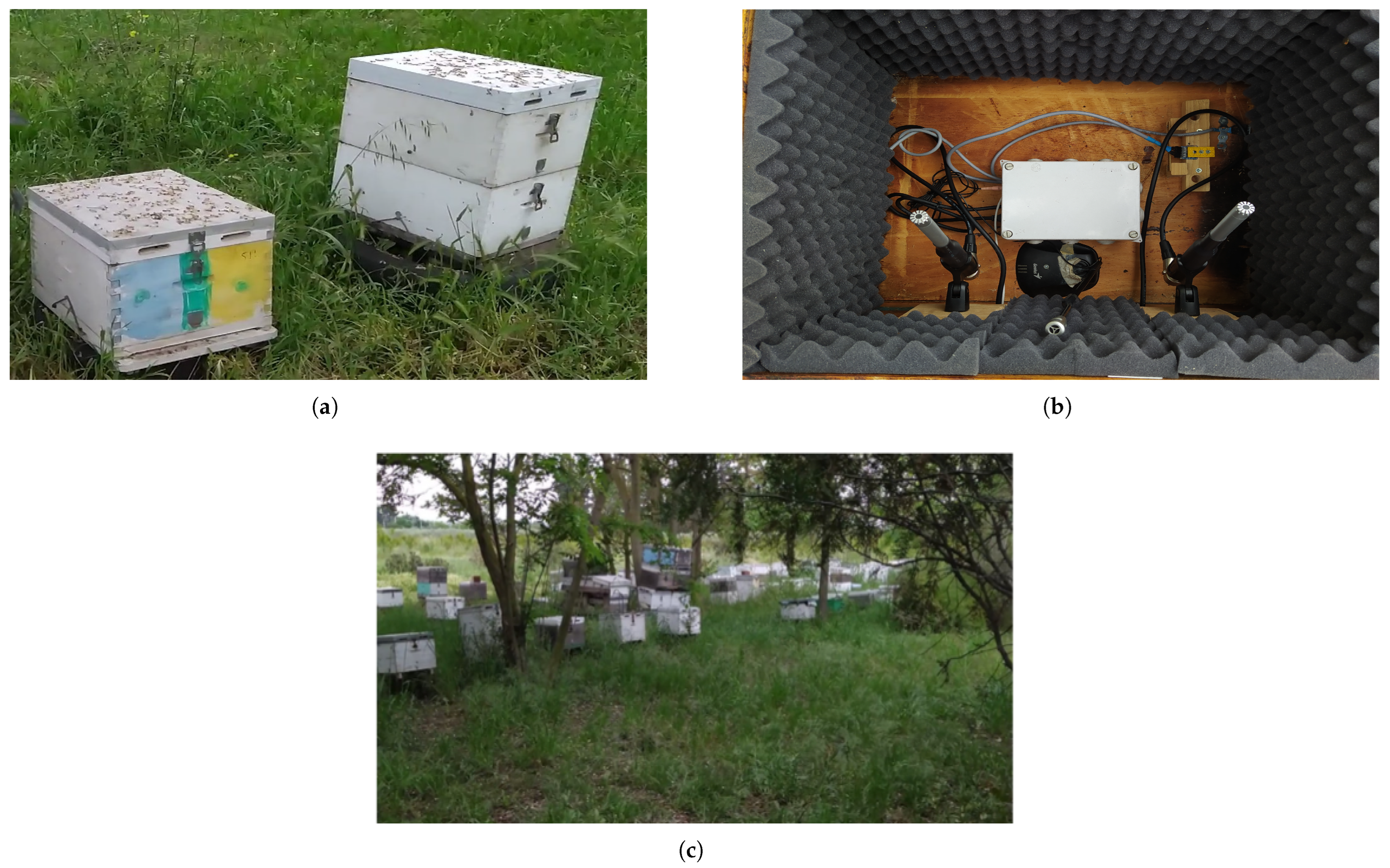
2.1. Dataset Acquisition

The experiment took place in the agricultural facilities of Aristotle University of Thessaloniki in Greece (Figure 1c), and it involves monitoring two beehives (hives m11 and m12) during their productive period of the year (May–August). During this period, each hive is forced into a queenless state by having the beekeepers remove the queen at specified dates. The hives were left queenless for a few days before introducing the queen again. This process was repeated two times for each hive, resulting in a dataset with four queenless periods and six healthy (before, in-between, and after the two queenless periods) in total for both hives [1].

Throughout the experimental process, the hives are equipped with an acquisition system, installed on a custom case on top of each hive. The system is equipped with Behringer ECM8000 microphones for sound recording and environmental sensors (BME280) monitoring the internal humidity, temperature, and pressure conditions. For this study’s purpose, only the sound recordings are considered.

The selected microphone, Behringer ECM8000, [31], is an Omnidirectional Condenser Microphone with 200 Ohms impedance. While its datasheet specifies sensitivity as 70 dB, an independent calibration report at 94 dB SPL/1 kHz [32] confirms −39.2 dB re 1 V/Pa (11 mV/Pa). Its frequency response spans the range of 20 Hz–20 kHz. The selected sound card Focusrite Scarlett’s [33], a 24-bit delta-sigma ADC that is combined with the microphone, provides an effective resolution of ∼18 bits. When paired with the Behringer ECM8000, the system’s practical resolution remains ADC-limited (∼18 bits) for typical recordings, making it suitable for 0–4 kHz voice, acoustic measurements, and music.

The recording of audio data is a fundamental process of the system and requires special attention to ensure the quality of the resulting recordings. This quality will entirely affect the processing stage, while the measurement environment is not particularly favorable.

For the proper positioning of the recording system, the monitored hives were customized appropriately. The customization included the use of a second empty hive placed on top of the hive under monitoring. This is a technique used by the beekeepers to house a hive with a larger population. In Figure 1a, two hives are on display. The hive on the left is a single-floor non-monitored beehive and the right hive is a modified dual-floor beehive under monitor. A metallic mesh was placed between the monitored and the empty hive to allow for sound diffusion, and the sound recording microphone was placed on the empty hive, Figure 1b. Also, absorption material was used for external environmental acoustic noise protection. This setup was implemented for two reasons. The first one is the sensitivity of the beehive to new modifications. Bee colonies generally oppose the alteration of the internal space of the hive. Consequently, there was not an option for a set-up inside the living colony and the proper placement of the systems in a parallel space, suitably isolated but with acoustic contact, was essential. The second one was for the protection of the systems from the activity of the bees as well as from the external environmental conditions.

The microphone is connected via wire to a computer equipped with the Focusrite Scarlet 8i6 external sound card, recording at a sampling rate of 44.1 kHz and a 16-bit resolution. The software used for sound capture is the REAPER Digital Audio Workstation (REAPER v6.09—27 April 2020). The system is able to monitor continuously throughout the experimental period. The gathered data was available online with the enabling of remote access.

As a result, there are sound recordings of the bees throughout the different phases that the hives are subjected to. Each hive experienced two orphan states, each preceded and followed by a healthy state. After the second orphan state, the hive was returned to a healthy condition and maintained as such. Thus, the sequence of states for each hive was as follows: first healthy state (Healthy A), first orphan state (Orphan A), second healthy state (Healthy B), second orphan state (Orphan B), and finally third healthy state (Healthy C). Each phase encompassed multiple days of sound recordings. From the raw sound recordings and after a feature extraction process that will be explained in Section 2.2, the final dataset consists of a set of features for every second of sound recordings and two classes representing the queenless and the healthy states. This dataset was utilized to train the machine learning models for the binary classification between these two states.

Although the number of hives in this study is limited (two hives), external acoustic noise is minimized through the use of sound-absorbing materials (Figure 1b), ensuring that the recorded signals predominantly reflect natural bee activity. The two hives are completely independent, with no shared biological factors that could confound the data. Furthermore, each hive underwent multiple transitions between “queenright” and “queenless” states at different chronological points, introducing temporal variability and enriching the dataset. This variability also contributes to the system’s resilience to real-world acoustic noise and environmental fluctuations.

By artificially inducing the “queenless” state, we were able to exert precise control over the timing and conditions of each hive’s transition. This controlled manipulation enabled accurate ground-truth labeling of hive status and facilitated the collection of clean, well-segmented data suitable for supervised machine learning tasks. Finally, our methodological design is consistent with recent studies in the field, where datasets are often limited to 2–6 hives [28,29,30] and the artificial induction of queenless states is a commonly employed practice [27,29].

2.2. Pre-Processing—Feature Extraction

The pre-processing steps involve the conversion of the raw audio data recorded from the microphones into a set of descriptive sound features, the MFCC. To achieve this, the raw data is first processed using multiple signal processing techniques, which are described below. Figure 2 presents an overview of the processing steps performed for the extraction of the MFCC. Note that different values for the pre-processing parameters were examined in order to determine the best parameter selection leading to the higher accuracy of the tested models. As a result, there are multiple variations of the original dataset with the MFCC features being calculated using different parameter values for each variation.

The process begins by resampling the raw data acquired with 44.1 kHz sampling rate to a lower frequency. This is done to reduce the data size and reduce calculation complexity and since only frequency ranges of up to 10 kHz are considered for this particular beekeeping phenomenon. The new sampling frequency (Fs) is one of the parameters that will be explored as described in

Table 1. The parameters used for feature extraction, leading to the four dataset configurations.

Dataset Configuration	Fs (Hz)	N_FFT	N_mels	Fmax (Hz)
config_0	4096	1024	9	60–2000
config_1	8192	1024	16	60–4000
config_2	8192	2048	32	60–4000
config_3	16384	2048	32	60–8000

.

The next step involves pre-emphasizing the higher frequency components of the acquired signals. This is a common technique that is performed to account for the increased attenuation of higher frequencies during the transmission of sound through different mediums. The lower frequencies suffer lower attenuation when traveling through objects than the higher frequencies. A pre-emphasis coefficient of 0.94 was selected to enhance higher frequencies and flatten the amplitudes of the frequency components. The resampled and pre-emphasized signal is then filtered through a linear FIR band-pass filter with 101 taps. The lower frequency limit of the filter was selected at 60 Hz to eliminate the noise components introduced by the power supply (220 V, 60 Hz). The higher limit was chosen as a parameter (Fmax), ranging from 2 kHz to 8 kHz, to examine the effectiveness of the models on data containing different frequency ranges.

The following step is the calculation of the STFT of the acquired signal. It involves windowing, framing, and shifting the signal and performing the FFT on each frame. The overall signal is divided into multiple overlapping frames ($50\%$ overlap) of a specified sample duration using a Hann window. For each frame, the FFT is calculated with a specified resolution (N_FFT) (see Table 1) that is used as a parameter. The result is a spectrogram with the frequency divided into N_FFT components, each with their corresponding amplitude. The time axis is divided into overlapping frames, with their duration in samples being chosen equal to the N_FFT resolution. Figure 3 demonstrates the power spectral density spectrograms for two acoustic measurements performed by the high-quality microphone. These are 1 h measurements recorded for a single hive during their healthy and orphan states. As indicated, the dominant frequency content is found in the below 2 kHz range, with a noticeable different acoustic signature between the two states. Figure 3 also exhibits the result of the pre-processing steps (filter and pre-emphasis) on the same signals. Notice that there is low-frequency noise (60 Hz) due to the power supply (220 V, 60 Hz) that was attenuated significantly with the filtering process.

For the extraction of the MFCC, the spectrogram is filtered through the mel filter banks, transforming it into the mel-spectrogram, a logarithmic spectral representation emphasizing lower frequencies in a similar way that humans perceive sound. The MFCC extraction process involves the use of triangular filters, each targeting a specific part of the spectrum, determined by the parameter N_mels and the lower (60 Hz) and upper frequency limits (Fmax), and then applying the Discrete Cosine Transform (DCT) [34]. For this study’s needs, four configurations were examined: (a) 9 mel bands in the 60–2000 Hz range, (b) 16 mel bands in the 60–4000 Hz range, (c) 32 mel bands in the 60–4000 Hz range, and (d) 32 mel bands in the 60–8000 Hz range (see Table 1). For each second of measurement, the MFCC are extracted for all the frames contained in that second, and then their median is calculated. The result is a feature space with N_mels features for each second of measurement indicating the median value for each mel band.

At this point, the processing steps for the extraction of the MFCC features are established. Throughout this process, parameters like the N_FFT resolution, the number (N_mel) of mel bands, the resampling frequency (Fs), and the upper frequency limit (Fmax) of the FIR filter are introduced as parameters. So, four different value combinations for these parameters are considered for this study, as described in Table 1, resulting in four different configurations of the same dataset. This was done to evaluate how these parameters affect the performance of the models and eventually select the configuration resulting in the best trade-off between accuracy and computational requirements. Table 1 also highlights the number of PCA components utilized for each configuration, which will be discussed in the following subsections.

2.3. Feature Importance

To estimate the importance of the MFCC features and consequently the contribution of each mel band to the final decision, Principal Component Analysis (PCA) was employed. This is a dimensionality reduction technique where the original feature space is transformed into an orthogonal vector space, with its eigenvectors being the Principal Components (PCs). Each PC is a linear combination of the original features and is ranked and ordered based on the variance they explain over the dataset. As a result, it is possible to accurately represent the majority of the dataset with only some of the first most important PCs, allowing for dimensionality reduction and simplification of the structure of high-dimensional data [35].

Apart from the dimensionality reduction, PCA can be used to indirectly infer the importance of the original features. This is done by examining the weights, or loadings, of each PC, indicating the contribution each feature has on that component [36]. To quantify the importance and account for the explained variance each PC has, the following equation was used:

$$\mathrm{Importance}\mathrm{Score}\left[n\right]=\sum _i^{N}P{C}_i\left[n\right]\times \mathrm{EVR}\left[i\right]$$

(1)

where n is the mel band index, N is the total number of PCs, $P{C}_i$ is the weight vector of each PC, and EVR is the explained variance ratio for each PC. As a result, for every dataset configuration, it is possible to identify which mel bands have a significant contribution and which do not. Apart from that, each MFFC or mel band is associated with a specific frequency range of the spectrum, which in turn highlights the significant frequency components considered to distinguish between the queenless and the queenright beehive states.

2.4. Machine Learning Approach

At this stage, the feature extraction method and the approach for determining feature importance are established. Subsequently, machine learning models are trained and evaluated using the queenright and queenless classes within the dataset. The models considered include Support Vector Machines (SVMs), Neural Networks (NNs), Logistic Regression (LR), and K-Nearest Neighbors (KNN). Various parameter combinations were tested for each model to identify the optimal configuration. Since four dataset configurations were examined, each model was evaluated across these configurations for each beehive, resulting in eight distinct test scenarios. This comprehensive evaluation allowed us to assess model consistency and identify the dataset configuration yielding the best performance.

Another important aspect of the approach that should be examined is the adaptability of the trained models to new datasets, as this can eventually dictate its applicability in real-world applications. This is because in real situations, the system is designed to be installed on completely unknown beehives without months of recordings available. For that matter, a Transfer Learning (TL) approach was followed, where the two best-performing models are trained on one hive (m12) and then fit on a very small percentage ($0.01\%$) of the other hive’s (m11) data. After this minimal training, the models are compared, and the one exhibiting the lowest drop in performance is selected to be implemented on the final system.

Considering that our machine learning (ML) problem is a binary classification task with two classes (queenright and queenless), we evaluate the models using well-established classification metrics, including class-wise precision, recall, and F1-score, as well as the average F1-score between the two classes [37]. The equations below describe these metrics in detail:

$$\begin{array}{cc}\hfill P_0& ={\displaystyle \frac{TN}{TN+FN}},P_1={\displaystyle \frac{TP}{TP+FP}}\left(a\right)\hfill \\ \hfill R_0& ={\displaystyle \frac{TN}{TN+FP}},R_1={\displaystyle \frac{TP}{TP+FN}}\left(b\right)\hfill \\ \hfill F{1}_0& ={\displaystyle \frac{2·P_0·R_0}{P_0+R_0}},F{1}_1={\displaystyle \frac{2·P_1·R_1}{P_1+R_1}}\left(c\right)\hfill \end{array}$$

(2)

In Equation (2), “0” represents the negative class (queenright), and “1” denotes the positive class (queenless). The terms TN and TP refer to true negative and true positive classifications, respectively, while FN and FP refer to false negative and false positive classifications, respectively.

For model evaluation, we primarily focus on the F1-score, as it provides a balance between precision and recall. The F1-score is particularly useful for imbalanced datasets, such as ours, where the data contains a higher number of queenright instances. This metric gives a more representative measure of model performance in such scenarios, compared to accuracy, which might be misleading due to the class imbalance [38].

2.5. Hardware Implementation

While accuracy of the models is critical, the model should be lightweight enough to be implemented in hardware with minimal resources. The targeted embedded system is the Arduino Zero (Arduino Srl, Somerville, MA, USA), equipped with the arm-cortex-m0 microprocessor. It is a system with limited processing power featuring a 32 KB memory but with limited power consumption requirements. According to the datasheet, a maximum value of 6.8 mA is reposted for active mode and a maximum value of 12.2 uA for the standby mode, both for room temperature. It is also equipped with a debugger that enables better monitoring and with multiple quality-of-life features provided by the Arduino platform.

For the embedded system sound recording, the Pulse-Density Modulation (PDM) Micro-Electro-Mechanical Systems (MEMS) Microphone of Adafruit was selected. The PDM MEMS Microphone, with omnidirectional sensitivity, is suitable for embedded applications and offers low power consumption. It has an acoustic overload point at 120 dBSPL and 61 dB signal-to-noise ratio. Since it provides digital PDM output, its sensitivity is—26 dBFS. The MP34DT01-M chip [39], which is the PDM microphone chip, uses a 1-bit sigma-delta modulator with oversampling, achieving an effective resolution of ∼10 bits (64 dB dynamic range). While the output is typically decimated to 16-bit PCM for compatibility, the true resolution is constrained by noise performance. This is sufficient for voice applications (0–4 kHz) but below high-fidelity audio standards.

To confirm the accurate recording of audio data, experiments were conducted using both the embedded system and a high-quality audio recording console. For the high-quality audio recording, the previously described setup was used, which included the Behringer ECM8000 microphone. For the purposes of implementation, experiments were carried out to assess the recording quality both in a laboratory environment and at the hive level, as depicted in Figure 4. The results of the experiments indicated a satisfactory frequency response of the recordings from the integrated system compared to the high-quality recordings, particularly in the frequency range of 10–1000 Hz.

Figure 5 illustrates the frequency content of the recording, derived from recordings with the following characteristics:

• high-quality sampling rate: 44.1 kHz;
• system sampling rate: 4–16 kHz;
• recording duration: 60 s;
• audio content: sounds of an active hive;
• placement of the two microphones (high-quality and system’s): in close proximity inside the hive;
• the analysis of the recordings was performed using the Welch method.

Figure 5. Power spectral density diagram of the high-quality recording system and the embedded system.

Figure 5. Power spectral density diagram of the high-quality recording system and the embedded system.

Figure 5 demonstrates a measurement of a healthy beehive recorded simultaneously with both the high-quality microphone and the embedded MEMS. This process was performed to ensure some level of consistency between the two microphones, especially for the low-frequency components. Specifically, we observe frequency content with similar power and shape across frequencies. More specifically, the PDM recording follows the frequency response of the high-quality recording for the range of 0–4096 Hz. The SNR of the system is tied to the SNR of characteristics of the PDM MEMS microphone. The maximum the embedded system supports is sampling rates up to 16 kHz but with a drop in quality as frequency increases. As a result, the use of the microphone through the embedded system was deemed satisfactory to capture low-frequency content up to 4 kHz. Also, the use of the Arduino Zero board for recording at the embedded system level proved to be an effective choice that also allowed for a relatively simple implementation in terms of complexity.

The operating cycle of the proposed system involves data sampling, data processing and feature extraction, the inference of the prediction model, the transmission of the result, and then entering low-power/sleep mode. Initially, the PDM MEMS microphone is activated to perform sound measurements of 1 s duration. During the recording, sound data is stored in a dedicated buffer in memory, with its size being dictated by the sampling rate of acquisition. The raw signal is then pre-processed to extract the features, and then the process continues with the inference of the trained models. The prediction result is then published for user access through the wireless transmission module, which is briefly activated to perform the transmission. The system then enters sleep mode for a specified duration (e.g., 10 min) until the process is initiated again.

Due to the limited capabilities of the hardware, a key concern is the memory requirements of the proposed approach as well as the processing time required for the feature extraction and inference of the implemented model. This is one of the reasons why multiple dataset configurations were examined, since an increase in FFT resolution or the number of mel bands or the complexity of the model, for example, could significantly increase the required memory and the processing time. These concerns were considered before making the final selection of dataset configuration and model selection. Additionally, there are optimized libraries (CMSIS) for digital signal processing and machine learning specifically developed for this series of arm processors that were employed to minimize the processing time and further optimize the process.

3. Results

This section presents the results that informed the final design decisions for the developed system.

3.1. PCA

After the feature extraction and the application of the PCA, it was possible to define the feature importance. More specifically, the mel bands responsible for most of the variance of the dataset can be established, as explained in the feature importance Section 2.3 of the Materials and Methods section. For this process, the fourth dataset configuration (config_03) was selected because of its filter ranges that include the largest part of the spectrum compared to the other configurations (60–8000 Hz), dividing it into 32 mel bands. As described in Section 2.3, to determine the importance of each mel-frequency band, we applied PCA to the config_03 dataset. For each mel band in the original dataset, we then calculated an importance score using Equation (1), where the component loadings and explained variance ratios were obtained using built-in functions from the scikit-learn python library [40]. Figure 6 is a graphical representation of these scores, with the seven most contributing mel bands (responsible for about $50\%$ of the variance) being highlighted.

Table 2. The seven most important mel bands representing about half of the overall variance.

Mel Band	Frequency Range (Hz)	Importance
mel_0	[56–240]	0.2013
mel_1	[144–336]	0.0973
mel_5	[504–688]	0.0444
mel_2	[232–424]	0.0438
mel_4	[416–600]	0.0343
mel_22	[2888–3488]	0.0327
mel_14	[1376–1664]	0.0303

presents these mel bands in descending order based on their importance along with their respective frequency range.

As outlined, mel band 0, which covers the frequency range 56–240 Hz, is the most important with an importance score of $0.2013$, followed by mel bands 1, 5, 2, 4, 22, and 14. Mel band 0 has an importance score that is almost $108\%$ higher than that of the second band, mel band 1. This result is expected, as the frequencies in mel band 0 encompass nearly all the frequencies associated with the “queenless” state (180 Hz, 225–285 Hz), as described in Section 1, while its center frequency (152 Hz) is close to 180 Hz, the primary frequency associated with the “queenless” state. Similarly, mel band 1, which spans from 144 to 336 Hz, includes all the frequencies of the “queenless” state, making these two mel bands the most significant. Following this, mel bands 5 and 4 predominantly cover frequencies associated with the “queenright” state, as described in Section 1, while mel band 2 encompasses both “queenless” and “queenright” state frequencies. Among the 32 extracted features, the mel bands mel_0 and mel_1 are identified as the most significant, as they encompass the frequency ranges produced by bees in the orphan state (225–285 Hz and 180 Hz). Additionally, the mel bands mel_1, mel_5, mel_2, and mel_4 are also highly important, as they correspond to the frequencies generated by bees in the normal state (300 Hz, 410 Hz, and 500 Hz).

3.2. ML Models Evaluation

We evaluate multiple machine learning (ML) models to identify the most optimal one, considering various factors such as performance and adaptability to previously unseen data. This section details the parameter tuning process and the evaluation of each tested model on the two hives under the four distinct configurations previously described. Each dataset is initially partitioned into a training set, comprising $80\%$ of the total data, and a testing set, comprising the remaining $20\%$. Parameter tuning is conducted separately for each dataset to ensure optimal model performance. The ML models assessed in this study include Support Vector Machines (SVMs), Neural Networks (NNs), Logistic Regression (LR), and K-Nearest Neighbors (KNN). To ensure robustness, the experiments were repeated ten times using different random seeds, and the average F1-scores from these runs are reported in the results.

A critical tuneable parameter for all ML models is the number of principal components (PCs) retained following Principal Component Analysis (PCA). Additionally, specific hyperparameters are optimized for each model: for KNN, the number of neighbors (k) is adjusted, while for NNs, both the number of layers in the network architecture and the number of training epochs are fine-tuned. Figure 7 presents the parameter tuning process for KNN and NNs using the first configuration dataset (config_0) with nine mel bands. As shown in Figure 7a, for both hives (m11, m12), selecting 9 principal components from PCA and 21 neighbors yielded the optimal performance. Increasing the number of neighbors led to excessive computational time or convergence failures, making such configurations unsuitable for consideration.

For the NN, various architectures are evaluated after training for the same number of epochs (85) by modifying the number of total layers. Our basic architecture is composed of fully connected (FC) layers. The first fully connected (FC) layer has dimensions $(\mathrm{PCs}\mathrm{number},64)$, while the final layer has dimensions $(16,1)$, with several intermediate layers in between. As illustrated in Figure 7b, the optimal architecture for both hives consists of four total FC layers. The respective intermediate FC layer sizes were (64, 32) and (32,16) [24,41]. Performance improvements tended to plateau beyond four layers, with deeper neural network architectures occasionally exhibiting declines in F1-score, likely due to increased model complexity and the risk of overfitting. Specifically, for hive M11, the F1-scores were 0.69 for the 2-layer model, 0.70 for the 3-layer model, 0.72 for both 4- and 5-layer models, and 0.71 for the 6-layer model, followed by a marked decrease to below 0.5 for architectures with 7 layers or more. In the case of hive M12, the F1-scores were 0.85 for the 2-layer model, 0.87 for the 3-layer model, and 0.90 for the 4-, 5-, 6-, and 8-layer models. Slight reductions were observed for the 7- and 10-layer models (0.89) and the 9-layer model (0.88). Figure 8 illustrates the complete neural network (NN) architecture adopted in this study. The ReLU activation function is applied to all layers except for the output layer, where the sigmoid activation function is utilized due to the binary classification nature of the problem.

Compared to other edge-oriented architectures, the proposed approach is simpler to implement and tune, requires minimal memory, and involves a relatively small number of parameters. For instance, both MobileNet [42] and MCUNet [43], architectures designed for deep-edge devices based on convolutional neural networks (CNNs) for computer vision tasks, comprise a large number of parameters (approximately 250 k and 500 k, respectively, while ours has approximately 1.5 k), rendering them unsuitable for our implementation. Similarly, TinyLSTM [44], although optimized for sequential time-series data on microcontrollers, is tailored to applications with strong temporal dependencies, resulting in elevated memory demands that exceed the constraints of our target platform (Arduino Zero). Lastly, while BinaryNet [45] achieves ultra-low-power inference through binary weights and activations, it necessitates specialized training regimes and toolchains, thereby introducing significant development overhead and tuning complexity.

For the training process, the binary cross-entropy loss function is employed, as it is specifically designed for binary classification tasks [46]. Equation (3) defines the adopted loss function, where $y_i$ represents the true label, ${\widehat{y}}_i$ denotes the predicted label, and N is the total number of samples. Finally, NN parameter tuning is performed by evaluating different numbers of principal components (PCs) in combination with an increasing number of training epochs. As illustrated in Figure 7c, the optimal configuration is determined to be six (6) PCs with 85 epochs for hive m11 and seven (7) PCs with 85 epochs for hive m12, both with learning rate (lr) 0.001. For the other ML models and datasets, similar Pareto-optimal tuning approaches are applied to identify the optimal number of PCs for each dataset, ensuring a balanced trade-off between performance and computational efficiency.

$$L=-{\displaystyle \frac{1}{N}}\sum _{i=1}^N\left(y_i\log \left({\widehat{y}}_i\right)+(1-y_i)\log \left(1-{\widehat{y}}_i\right)\right)$$

(3)

Next, we present the experimental results for the optimal parameter set of each machine learning (ML) model across all data configurations. Figure 9 illustrates the average F1-score for each scenario using the datasets from hives m11 and m12. The analysis is conducted in two stages: first, we compare the performance of different data configurations for each ML model, and subsequently, we compare the performance of the different ML models.

For the m11 dataset, as shown in Figure 9, the optimal configuration for KNN and Logistic Regression is config_3, yielding an average F1-score approximately $13\%$ higher than the lowest-performing configuration (config_0). In contrast, for SVM and NN, the optimal configuration is config_2, demonstrating improvements of $15\%$ and $22\%$, respectively, over the worst-performing configuration (config_0). For the m12 dataset, config_2 is identified as the optimal configuration across all ML models, resulting in an average F1-score improvement of 4–$8.5\%$ compared to the lowest-performing configurations. Specifically, for KNN, the worst performance is observed in config_0, while for all other ML models, config_1 is the least effective configuration. As described in Table 1, config_0 includes the fewest number of mel bands (9), providing limited options for Principal Component Analysis (PCA), thereby making it the weakest data configuration, as the results also suggest. On the other hand, config_2 and config_3 both include 32 mel bands, making them superior data configurations for all use cases. Specifically, config_2 is generally the better configuration, as indicated by the results, which is expected considering its lower resampling frequency, leading to a more manageable dataset. For the model comparison, the optimal ML model for the m11 dataset is the Neural Network (NN), achieving an average F1-score of 0.85, followed closely by KNN with an average F1-score of 0.84. For the m12 dataset, KNN emerges as the best-performing model, attaining an average F1-score of 0.97, followed by NN with an average F1-score of 0.92.

Table 3. Analytic performance results for the NN classifier.

Dataset Configuration	Hive	Precision (Class 0)	Recall (Class 0)	F1-Score (Class 0)	Precision (Class 1)	Recall (Class 1)	F1-Score (Class 1)	Average F1
config_0	m11	0.84	0.90	0.87	0.63	0.49	0.55	0.81
	m12	0.88	0.91	0.90	0.84	0.79	0.82	0.87
config_1	m11	0.85	0.91	0.88	0.67	0.54	0.60	0.81
	m12	0.91	0.95	0.93	0.83	0.71	0.77	0.89
config_2	m11	0.86	0.93	0.89	0.73	0.56	0.64	0.83
	m12	0.93	0.96	0.95	0.87	0.80	0.84	0.92
config_3	m11	0.86	0.95	0.90	0.78	0.56	0.65	0.85
	m12	0.92	0.96	0.94	0.85	0.76	0.80	0.90

presents the detailed performance results of the Neural Network (NN) model across all data configurations for both the m11 and m12 datasets. As shown, class 0 (queenright) consistently achieves higher scores compared to class 1 (queenless), which is expected given the larger proportion of queenright data in both the training and testing sets. For the m11 dataset, class-wise performance improves as the complexity of the data configuration increases, with config_3 identified as the optimal configuration for both classes, yielding F1-scores of 0.90 and 0.65 for class 0 and class 1, respectively. Notably, class 0 exhibits minimal improvement across configurations due to its already high performance, whereas class 1 shows a significant $18\%$ improvement. For the m12 dataset, the optimal configuration is config_2 for both classes, with F1-scores of 0.95 and 0.84 for class 0 and class 1, respectively. Similar to the m11 dataset, the performance of class 1 improves more substantially compared to class 0.

Finally, we evaluate the adaptability of the two best-performing ML models, Neural Networks (NN) and K-Nearest Neighbors (KNN), on previously unseen data. To achieve this, we employ the transfer learning (TL) technique between the two hives, m11 and m12. Specifically, we use the m12 dataset as the original (source) dataset, where the models are initially trained as previously described, for 85 epochs for NN and with k = 21 for KNN. Subsequently, the pre-trained models are fine-tuned on a small subset of m11 data before being tested on the full m11 dataset to assess their generalization capability. The training process involves using $80\%$ of m12 data for training and $20\%$ for testing. After applying TL, only $0.01\%$ of m11 data is used for fine-tuning, while $20\%$ of the remaining m11 data is allocated for testing.

Table 4. Results of the transfer learning process for the two best-performing models.

Model	Average F1-Score (Original Dataset, m12)	Average F1-Score (New Dataset with TL, m11)
NN	0.91	0.82
KNN	0.94	0.81

presents the experimental results, demonstrating that the NN model achieves an average F1-score of 0.91 on the original (m12) dataset and 0.82 on the unseen (m11) dataset, corresponding to a $9.8\%$ performance drop. In contrast, KNN reaches an average F1-score of 0.94 on the original dataset and 0.81 on the unseen dataset, exhibiting a $13.8\%$ performance drop. These findings indicate that while both models exhibit adaptability to new data, NN demonstrates a more stable performance under transfer learning conditions compared to KNN.

3.3. Hardware Implementation

The main processing tasks during runtime are the pre-processing of the raw audio data for the extraction of the MFCC features along with the PCA transformation and the inference of the NN. At this point, based on the model evaluation process, the accuracy of each configuration was tested, with config_2 demonstrating the most consistent results between the two hives. Apart from that, it provides adequate spectral resolution (2048-point FFT with 32 mel bands) covering frequency components in the range of 60–4000 Hz (due to the 8192 Hz sampling rate—see Table 1), which is where the beekeeping sound phenomena recede. However, each configuration is linked with different memory requirements and processing times, which is important to examine due to the minimal resources of the targeted hardware platform (Arduino Zero and arm-cortex-m0-plus processor).

Given the memory restrictions (32 KB), the feature extraction process had to be optimized in terms of memory. For that matter, the FIR filter coefficients, the Hanning window, and the mel filter banks coefficients had to be pre-calculated for each configuration along with a look-up table for the DCT calculation. This approach is reasonable given that these arrays are constant throughout the process and enable them to be stored into flash memory instead of the limited RAM. For the analysis, the CMSIS-DSP optimized functions for MFCC extraction (16-bit precision) were utilized along with its optimized matrix multiplication functions for windowing, FIR, and PCA calculations.

For the inference, the targeted model is the one described in the previous subsection, the NN with four FC layers (Figure 8). The KNN alternative was eventually discarded due to the lesser transfer learning capabilities and because of the implementation nature of such algorithms that require storing a large chunk of the dataset into memory. This NN architecture was employed for all four configurations but with each one having a different number of input features on their first FC layer. The extracted weights and biases from the training process were quantized with 8-bit precision, further minimizing the memory requirements of the models. After the quantization, the F1-score drop was negligible, as it was <$0.1$ in all cases. A single scratch buffer was utilized for all four layers of the network, and the analysis was implemented utilizing the CMSIS-NN optimized function for FC layers, which requires storing the weight values in an interleaved format. This ensures the weights are accessed from memory in the correct order for the internal matrix multiplications, minimizing cache misses and optimizing processing speed. Implementing the NN with quantized weights is associated with a drop in accuracy that was negligible in the current implementation.

The results of the implementation process involve capturing the memory utilization and processing time required for each configuration to run on the hardware platform.

Table 5. Memory requirements and processing time for the feature extraction and the inference of the NN model on the different dataset configurations.

Data	Feature Extraction		Inference
	Memory (kB)	Processing Time (ms)	Memory (kB)	Processing Time (ms)
config_0	$12.272$	$0.408428$	$3.196$	$0.000990$
config_1	$13.312$	$0.822912$	$3.212$	$0.001113$
config_2	$20.576$	$0.827076$	$3.212$	$0.001183$
config_3	$20.592$	$1.656056$	$3.228$	$0.001316$

presents these results for the feature extraction and inference. The feature extraction was the most demanding both in terms of memory and processing time. Its processing time is associated with extracting the features for a full 1 s of audio data. As a result, the window length (which is equal to N_FFT in all cases), and the sampling rate determine the number of processed frames in each second. This is the reason that some configurations exhibit significantly longer processing times. The main parameter affecting memory requirements in feature extraction is the N_FFT resolution. As indicated in Table 1, configs_0–1 and configs_2–3 have 1024 and 2048-point resolution, respectively, leading to memory capacity that is almost twice as large (Table 5). Focusing on config_2, which was the choice based on the model evaluations, the processing time is reasonable, needing approximately 0.827 s to process 1 s of measurement, as well as the memory leaves room of approximately 12 KB for the inference and other potential utilities.

For the NN inference, the processing times and memory requirements are significantly lower and with minor variations between configurations since only one FC layer differentiates between each case. All configurations require around $3.2$ KB of memory, which even for the most resource-intensive configurations (config_2 and config_3) utilizes a total of around 23.8 KB out of the 32 KB of RAM. The processing times are almost negligible compared to the feature extraction process, indicating the efficiency of the CMSIS-NN optimized functions for FC layers and activation functions.

4. Discussion and Conclusions

Throughout this study, the whole process of the proposed approach was exhibited, from the experimental procedure and the setup for data acquisition to the feature extraction calculations, the feature importance, the model training, parameter-tuning and evaluation process, as well as the hardware implementation. Throughout this whole pipeline, different configurations of parameter values were examined, leading to the choice of config_2 with the FC NN architecture demonstrated in Figure 8.

More specifically, through the feature extraction and the PCA processes, it was possible to evaluate the importance of the MFCC features. As a result, it was exhibited that the most dominant mel bands (based on the explained variance of the dataset) correspond to the mel bands of Table 2 and are linked to the lower part of the spectrum, as suggested by the literature, namely centered around frequencies 152, 240, 328, 504, 600, 1520, and 3176 Hz. As outlined by the model evaluation process, by considering model accuracy on different dataset configurations, parameter values, and models, both the KNN and NN were reasonable choices. The NN, however, exhibited a lower drop in accuracy during the TL process compared to the KNN. This fact, along with the large memory requirements required for implementing a KNN, which is a prohibiting factor for a low-resource embedded system, discarded the KNN scenario.

Apart from that, as exhibited through the hardware implementation, all configurations were successfully deployed on the targeted platform with acceptable processing times and memory requirements. The NN architecture proved lightweight enough, highlighting the efficiency of the optimized arm libraries. The choice of config_2 results in a total RAM requirement of around 24 KB, leaving enough room for additional functionalities and utilities. Fully processing and inferencing an audio signal of 1 s duration requires approximately 0.83 s. In a practical setting, this means that the proposed system can activate from its sleep routine, acquire 1 s of data, spend 0.83 s to process and decide whether the queen is absent, and then return to sleep. This scenario can be utilized successfully, especially in off-the-grid cases and low-energy scenarios.

For future development of the proposed approach, the dataset could be enhanced by including audio measurements of additional beekeeping phenomena (swarming, arrhenotoky), and by considering multiple modalities apart from sound (temperature, pressure, etc.). Apart from the MFCC features, more signal-processing techniques or deep learning approaches for feature extraction could be explored to eventually compare the accuracy of different feature configurations. Even for the MFCC features, different granularities and parameters could be explored, further highlighting the underlying characteristics of bees’ sound. As for the model evaluation, while this study focused on low-level models with minimal requirements, more advanced architectures and time series forecasting methods could be also explored. Further evaluation under explicitly controlled acoustic interference conditions, such as wind, rain, human activity, and insect noise, could also be incorporated to systematically assess the model’s robustness to external acoustic disturbances.

To conclude, we propose an IoT-based system for data collection, monitoring, and analysis of beehive conditions, utilizing multiple sensors to measure key metrics such as acoustic signals, temperature, and humidity. Acoustic data is transformed into mel-spectrograms and analyzed with machine learning (ML) models to detect queenless states. We evaluated several ML models across two hives and four sampling frequencies, optimizing parameters via Pareto analysis for each dataset. Neural networks (NNs) emerged as the best-performing model, achieving F1-scores of 0.85 and 0.92 on hives M11 and M12, respectively, while maintaining low memory usage. The NN also generalized effectively to unseen data through transfer learning, requiring fine-tuning on only $0.01\%$ of new samples. Deployment on an Arduino Zero demonstrated real-time capability, with the system acquiring and processing 1 s of data records in $0.83$ s before returning to sleep, suitable for off-grid, low-power applications.

References

1. Kanelis, D.; Liolios, V.; Papadopoulou, F.; Rodopoulou, M.A.; Kampelopoulos, D.; Siozios, K.; Tananaki, C. Decoding the Behavior of a Queenless Colony Using Sound Signals. Biology 2023, 12, 1392. [Google Scholar] [CrossRef] [PubMed]
2. Albayrak, A.; Çeven, S.; Bayır, R. Modeling of migratory beekeeper behaviors with machine learning approach using meteorological and environmental variables: The case of Turkey. Ecol. Inform. 2021, 66, 101470. [Google Scholar] [CrossRef]
3. Kaplan Berkaya, S.; Sora Gunal, E.; Gunal, S. Deep learning-based classification models for beehive monitoring. Ecol. Inform. 2021, 64, 101353. [Google Scholar] [CrossRef]
4. Hrncir, M.; Friedrich, B.; Juergen, D. Vibratory and Airborne-Sound Signals in Bee Communication (Hymenoptera). In Insect Sounds and Communication: Physiology, Behaviour, Ecology, and Evolution; Drosopoulos, S., Claridge, M.F., Eds.; CRC Press: Boca Raton, FL, USA, 2006; pp. 421–422. [Google Scholar]
5. Nolasco, I.; Benetos, E. To bee or not to bee: Investigating machine learning approaches for beehive sound recognition. In Proceedings of the Proceedings of the Detection and Classification of Acoustic Scenes and Events Workshop (DCASE2018), Surrey, UK, 19–20 November 2018. [Google Scholar]
6. Dietlein, D.G. A method for remote monitoring of activity of honeybee colonies by sound analysis. J. Apic. Res. 1985, 24, 176–183. [Google Scholar] [CrossRef]
7. Uthoff, C.; Homsi, M.N.; von Bergen, M. Acoustic and vibration monitoring of honeybee colonies for beekeeping-relevant aspects of presence of queen bee and swarming. Comput. Electron. Agric. 2023, 205, 107589. [Google Scholar] [CrossRef]
8. Qandour, A.; Ahmad, I.; Habibi, D.; Leppard, M. Remote beehive monitoring using acoustic signals. Acoust. Aust. 2014, 42, 204–209. [Google Scholar]
9. Fahrenholz, L.; Lamprecht, I.; Schricker, B. Calorimetric investigations of the different castes of honey bees, Apis mellifera carnica. J. Comp. Physiol. B 1992, 162, 119–130. [Google Scholar] [CrossRef]
10. Bell, H.; Kietzman, P.; Nieh, J. The Complex World of Honey Bee Vibrational Signaling: A Response to Ramsey et al. (2017). arXiv 2024, arXiv:2408.14430. [Google Scholar]
11. Greggers, U.; Koch, G.; Schmidt, V.; Dürr, A.; Floriou-Servou, A.; Piepenbrock, D.; Göpfert, M.C.; Menzel, R. Reception and learning of electric fields in bees. Proc. R. Soc. B Biol. Sci. 2013, 280, 20130528. [Google Scholar] [CrossRef]
12. Liao, Y.; McGuirk, A.; Biggs, B.; Chaudhuri, A.; Langlois, A.; Deters, V. Noninvasive Beehive Monitoring Through Acoustic Data Using SAS® Event Stream Processing and SAS® Viya®; Technical report; SAS Institute Inc.: Belgrade, Serbia, 2020. [Google Scholar]
13. Cejrowski, T.; Szymanski, J.; Mora, H.; Gil, D. Detection of the bee queen presence using sound analysis. In Proceedings of the Asian Conference on Intelligent Information and Database Systems, Dong Hoi City, Vietnam, 19–21 March 2018; pp. 297–306. [Google Scholar]
14. Phan, T.T.H.; Nguyen, H.D.; Nguyen, D.D. Evaluation of Feature Extraction Methods for Bee Audio Classification. In Intelligence of Things: Technologies and Applications; Nguyen, N.T., Dao, N.N., Pham, Q.D., Le, H.A., Eds.; Springer: Cham, Switzerland, 2022; pp. 194–203. [Google Scholar]
15. Polyniak, Y.; Fedasyuk, D.; Marusenkova, T. Identification of Bee Colony Acoustic Signals using the Dynamic Time Warping Algorithm. ECONTECHMOD Int. Q. J. Econ. Technol. Model. Process 2019, 8, 19–27. [Google Scholar]
16. Cecchi, S.; Spinsante, S.; Terenzi, A.; Orcioni, S. A Smart Sensor-Based Measurement System for Advanced Bee Hive Monitoring. Sensors 2020, 20, 2726. [Google Scholar] [CrossRef]
17. Andrijević, N.; Urošević, V.; Arsić, B.; Herceg, D.; Savić, B. IoT Monitoring and Prediction Modeling of Honeybee Activity with Alarm. Electronics 2022, 11, 783. [Google Scholar] [CrossRef]
18. Ngo, T.N.; Wu, K.C.; Yang, E.C.; Lin, T.T. A real-time imaging system for multiple honey bee tracking and activity monitoring. Comput. Electron. Agric. 2019, 163, 104841. [Google Scholar] [CrossRef]
19. Voudiotis, G.; Kontogiannis, S.; Pikridas, C. Proposed Smart Monitoring System for the Detection of Bee Swarming. Inventions 2021, 6, 87. [Google Scholar] [CrossRef]
20. Voudiotis, G.; Moraiti, A.; Kontogiannis, S. Deep Learning Beehive Monitoring System for Early Detection of the Varroa Mite. Signals 2022, 3, 506–523. [Google Scholar] [CrossRef]
21. Mrozek, D.; Gorny, R.; Wachowicz, A.; Małysiak-Mrozek, B. Edge-Based Detection of Varroosis in Beehives with IoT Devices with Embedded and TPU-Accelerated Machine Learning. Appl. Sci. 2021, 11, 1078. [Google Scholar] [CrossRef]
22. Ngo, T.N.; Rustia, D.J.A.; Yang, E.C.; Lin, T.T. Automated monitoring and analyses of honey bee pollen foraging behavior using a deep learning-based imaging system. Comput. Electron. Agric. 2021, 187, 106239. [Google Scholar] [CrossRef]
23. Kulyukin, V. Audio, Image, Video, and Weather Datasets for Continuous Electronic Beehive Monitoring. Appl. Sci. 2021, 11, 4632. [Google Scholar] [CrossRef]
24. De Simone, A.; Barbisan, L.; Turvani, G.; Riente, F. Advancing Beekeeping: IoT and TinyML for Queen Bee Monitoring Using Audio Signals. IEEE Trans. Instrum. Meas. 2024, 73, 2527309. [Google Scholar] [CrossRef]
25. Otesbelgue, A.; de Lima Rodrigues, Í.; dos Santos, C.F.; Gomes, D.G.; Blochtein, B. The missing queen: A non-invasive method to identify queenless stingless bee hives. Apidologie 2025, 56, 28. [Google Scholar] [CrossRef]
26. Maralit, A.D.; Imperial, A.A.; Cayangyang, R.T.; Tan, J.B.; Maaño, R.A.; Belleza, R.C.; De Castro, P.J.C.; Oreta, D.E.S. QueenBuzz: A CNN-based architecture for Sound Processing of Queenless Beehive Towards European Apis Mellifera Bee Colonies’ Survivability. In Proceedings of the 2023 International Conference on Computer Science, Information Technology and Engineering (ICCoSITE), Jakarta, Indonesia, 16 February 2023; pp. 691–696. [Google Scholar] [CrossRef]
27. Doinea, M.; Trandafir, I.; Toma, C.V.; Popa, M.; Zamfiroiu, A. IoT Embedded Smart Monitoring System with Edge Machine Learning for Beehive Management. Int. J. Comput. Commun. Control 2024, 19, 632. [Google Scholar] [CrossRef]
28. Kulyukin, V.; Mukherjee, S.; Amlathe, P. Toward Audio Beehive Monitoring: Deep Learning vs. Standard Machine Learning in Classifying Beehive Audio Samples. Appl. Sci. 2018, 8, 1573. [Google Scholar] [CrossRef]
29. Ruvinga, S.; Hunter, G.; Duran, O.; Nebel, J.C. Identifying Queenlessness in Honeybee Hives from Audio Signals Using Machine Learning. Electronics 2023, 12, 1627. [Google Scholar] [CrossRef]
30. Ruvinga, S.; Hunter, G.J.; Duran, O.; Nebel, J.C. Use of LSTM Networks to Identify “Queenlessness” in Honeybee Hives from Audio Signals. In Proceedings of the 2021 17th International Conference on Intelligent Environments (IE), Dubai, United Arab Emirates, 21–24 June 2021; pp. 1–4. [Google Scholar] [CrossRef]
31. Music Group Ltd. ECM8000 Technical Specifications: Ultra-Linear Measurement Condenser Microphone; Behringer: Willich, Germany, 2013; Datasheet; Available online: https://cdn.mediavalet.com/aunsw/musictribe/ri9AgIhkSkeKygnwBCmTbQ/QNqLVKUimkqAIilLXp9r3Q/Original/ECM8000_P0118_S_EN.pdf (accessed on 22 July 2025).
32. Cross Spectrum Labs. Microphone Frequency Response Measurement Report; Cross Spectrum Labs: Burlington, MA, USA, 2011; Report; Available online: https://www.cross-spectrum.com/cslmics/001_mic_report.pdf (accessed on 23 July 2025).
33. Focusrite Audio Engineering Limited. Scarlett 2i2 (3rd Gen) User Guide, 2nd ed.; Focusrite: High Wycombe, UK, 2021; Available online: https://fael-downloads-prod.focusrite.com/customer/prod/downloads/Scarlett%202i2%203rd%20Gen%20User%20Guide%20V2.pdf (accessed on 22 July 2025).
34. Molau, S.; Pitz, M.; Schluter, R.; Ney, H. Computing mel-frequency cepstral coefficients on the power spectrum. In Proceedings of the 2001 IEEE International Conference on Acoustics, Speech, and Signal Processing, Salt Lake City, UT, USA, 7–11 May 2001; Proceedings (cat. No. 01CH37221). IEEE: Piscataway, NJ, USA, 2001; Volume 1, pp. 73–76. [Google Scholar]
35. Giordani, P. Principal component analysis. In Encyclopedia of Social Network Analysis and Mining; Springer: Berlin/Heidelberg, Germany, 2018; pp. 1831–1844. [Google Scholar]
36. Odhiambo Omuya, E.; Onyango Okeyo, G.; Waema Kimwele, M. Feature Selection for Classification using Principal Component Analysis and Information Gain. Expert Syst. Appl. 2021, 174, 114765. [Google Scholar] [CrossRef]
37. Sokolova, M.; Lapalme, G. A systematic analysis of performance measures for classification tasks. Inf. Process. Manag. 2009, 45, 427–437. [Google Scholar] [CrossRef]
38. He, H.; Garcia, E.A. Learning from Imbalanced Data. IEEE Trans. Knowl. Data Eng. 2009, 21, 1263–1284. [Google Scholar] [CrossRef]
39. STMicroelectronics. MP34DT01-M: MEMS Audio Sensor Omnidirectional Digital Microphone, 3rd ed.; STMicroelectronics: Geneva, Switzerland, 2014; Datasheet; Available online: https://www.st.com/resource/en/datasheet/mp34dt01-m.pdf (accessed on 23 July 2025).
40. Pedregosa, F.; Varoquaux, G.; Gramfort, A.; Michel, V.; Thirion, B.; Grisel, O.; Blondel, M.; Prettenhofer, P.; Weiss, R.; Dubourg, V.; et al. Scikit-learn: Machine Learning in Python. J. Mach. Learn. Res. 2011, 12, 2825–2830. [Google Scholar]
41. Quaderi, S.J.; Labonno, S.; Mostafa, S.; Akhter, S. Identify The Beehive Sound Using Deep Learning. arXiv 2022, arXiv:2209.01374. [Google Scholar] [CrossRef]
42. Howard, A.G. Mobilenets: Efficient convolutional neural networks for mobile vision applications. arXiv 2017, arXiv:1704.04861. [Google Scholar] [CrossRef]
43. Lin, J.; Chen, W.M.; Lin, Y.; Gan, C.; Han, S. Mcunet: Tiny deep learning on iot devices. Adv. Neural Inf. Process. Syst. 2020, 33, 11711–11722. [Google Scholar]
44. Fedorov, I.; Stamenovic, M.; Jensen, C.; Yang, L.C.; Mandell, A.; Gan, Y.; Mattina, M.; Whatmough, P.N. TinyLSTMs: Efficient neural speech enhancement for hearing aids. arXiv 2020, arXiv:2005.11138. [Google Scholar] [CrossRef]
45. Courbariaux, M.; Hubara, I.; Soudry, D.; El-Yaniv, R.; Bengio, Y. Binarized neural networks: Training deep neural networks with weights and activations constrained to+ 1 or-1. arXiv 2016, arXiv:1602.02830. [Google Scholar]
46. Terven, J.; Cordova-Esparza, D.M.; Ramirez-Pedraza, A.; Chavez-Urbiola, E.A.; Romero-Gonzalez, J.A. Loss functions and metrics in deep learning. arXiv 2023, arXiv:2307.02694. [Google Scholar] [CrossRef]
Figure 1. (a) Single-floor beehive without monitoring system (left) and modified dual-floor beehive (right) with the monitoring system; (b) high-quality recording system installed in a specially configured hive chamber; (c) section of the agricultural facilities at Aristotle University of Thessaloniki, Greece, where the experiment was conducted.
Electronics 14 02959 g001
Figure 2. Processing steps for extracting the Normalized MFCC features from the raw audio signal.
Electronics 14 02959 g002
Figure 3. Spectrograms of the raw and pre-processed signals from the healthy and orphan beehive.
Electronics 14 02959 g003
Figure 4. High-quality recording system and microphone-based embedded system in specially configured hive chamber.
Electronics 14 02959 g004
Figure 6. Graphical representation of the importance scores of each mel band.
Electronics 14 02959 g006
Figure 7. Parameter tuning results for different models. The solid lines with dots correspond to hive  m11, and the dashed lines with x to hive  m12. (a) KNN parameter tuning showing average F1-scores across different numbers of neighbors for varying numbers of principal components (PCs). (b) Neural network architecture tuning. (c) Neural network parameter tuning showing the impact of epochs on performance across different numbers of PCs.
Electronics 14 02959 g007
Figure 8. Graphical representation of adopted NN architecture.
Electronics 14 02959 g008
Figure 9. Graphical representation of average F1-score for different ML models and data configurations.
Electronics 14 02959 g009