SS-LIO: Robust Tightly Coupled Solid-State LiDAR–Inertial Odometry for Indoor Degraded Environments

Abstract

Solid-state LiDAR systems are widely recognized for their high reliability, low cost, and lightweight design, but they encounter significant challenges in SLAM tasks due to their limited field of view and uneven horizontal scanning patterns, especially in indoor environments with geometric constraints. To address these challenges, this paper proposes SS-LIO, a precise, robust, and real-time LiDAR–Inertial odometry solution designed for solid-state LiDAR systems. SS-LIO uses uncertainty propagation in LiDAR point-cloud modeling and a tightly coupled iterative extended Kalman filter to fuse LiDAR feature points with IMU data for reliable localization. It also employs voxels to encapsulate planar features for accurate map construction. Experimental results from open-source datasets and self-collected data demonstrate that SS-LIO achieves superior accuracy and robustness compared to state-of-the-art methods, with an end-to-end drift of only 0.2 m in indoor degraded scenarios. The detailed and accurate point-cloud maps generated by SS-LIO reflect the smoothness and precision of trajectory estimation, with significantly reduced drift and deviation. These outcomes highlight the effectiveness of SS-LIO in addressing the SLAM challenges posed by solid-state LiDAR systems and its capability to produce reliable maps in complex indoor settings.

1. Introduction

In recent years, accurate real-time state estimation and mapping have become crucial for mobile robots to effectively sense, plan, and navigate in unknown environments. Vision-based simultaneous localization and mapping (SLAM) [1,2,3] has shown remarkable performance in localization accuracy. However, these methods are often constrained by their reliance on sparse feature maps, making them vulnerable to lighting changes and motion blur. Furthermore, the limited computational resources on mobile robots pose a significant challenge to achieving real-time dense mapping with high resolution and accuracy [4].

In recent years, faced with the challenges posed by lighting variations and motion blur, the research community has increasingly turned its attention to LiDAR odometry (LO) [5,6,7] and LiDAR–Inertial odometry (LIO) [8,9,10,11,12,13,14]. These methods have demonstrated significant advantages over their vision-based counterparts, particularly in terms of real-time processing and accuracy. By leveraging LiDAR’s exceptional capacity for distance measurement and depth perception, LO and LIO algorithms have established themselves as powerful alternatives in the field of SLAM [8,10,11,12]. LiDAR’s capability to provide precise ambient distance data, in combination with the IMU’s ability to deliver accurate and environmentally independent short-term motion information, underscores the unique strengths of each technology. Building on these complementary capabilities, LiDAR and IMU sensor-based applications have become increasingly prevalent in SLAM tasks, driving the emergence and development of LiDAR–Inertial odometry as a robust solution for addressing the limitations of traditional vision-based approaches.

Although LIO methods excel in computational efficiency, mismatches between scanned data and target maps frequently occur during operation. Early research primarily focused on extracting geometric feature points [9,15,16], and then matched the data with the nearest neighboring as well as the Kalman filter [10,11,12,17]. However, the degradation challenge in LIO has emerged as a critical issue for high performance of SLAM, because of sense noise, environmental impact, and scanned data association error. For instance, robots often struggle to estimate their motion accurately along the wall in confined spaces such as narrow corridors or environments with dominant single walls. To address this issue, some research has employed probabilistic models to represent target maps, such as modeling them as planar [18] or curved elements [19,20]. Using these models, matching relationships with high uncertainty are effectively mitigated during the pose estimation process, thereby enhancing the accuracy of the matching. Nevertheless, for indoor environments, the degradation issue still exits, and is worth further investigation.

In this work, an accurate, robust, and real-time LIO approach is specifically designed for solid-state LiDAR systems. The key contributions are as follows:

(1)

A probabilistic model for planar elements is built for mitigating degradation effects.

(2)

A tightly coupled iterative extended Kalman filter with an IMU is employed to integrate LiDAR feature points with IMU data, thus alleviating the issue of geometric degradation

(3)

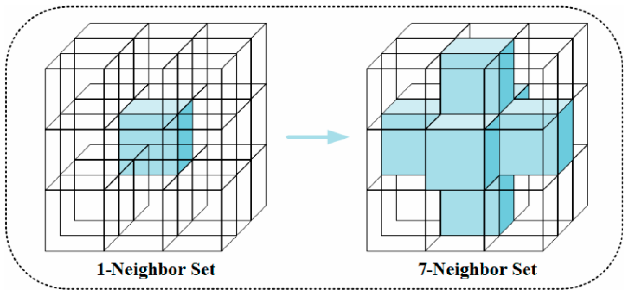
A set of voxels which contain planar features for generating a new map is formed by facilitating probabilistic and precise alignment of LiDAR scans with the environment.

The organization of this paper is as follows: in Section 2, several related works are introduced, and a tightly coupled LIO for indoor degraded environments, named as SS-LIO, is described in Section 3. In Section 4, the experimental results are presented, and the performance of the proposed method is then compared with that of similar methods to demonstrate its effectiveness in the degradation of LIO. Finally, conclusions are drawn in Section 5.

2. Related Work

2.1. LiDAR (-Inertial) Odometry

In the realm of LiDAR (-inertial) odometry for SLAM, two primary categories exist: indirect and direct methods. The distinction between these approaches lies in their processing of point-cloud data. Indirect methods require initial feature extraction from point clouds, while direct methods utilize the entire voxelized point cloud for attitude estimation.

LOAM [15] is a seminal indirect method capable of real-time mapping. It begins by extracting edge and planar features from the point-cloud data. After feature extraction, coarse positioning is achieved through two high-frequency odometers, while fine positioning is accomplished via map-matching. Building on this foundation, LeGO-LOAM [9] was developed as a lightweight, ground-optimized LiDAR odometry and mapping approach. By leveraging ground information, it enhances the robustness and efficiency of attitude estimation. LiLi-OM [21] addresses the irregular scan pattern of the Livox Horizon solid-state LiDAR by introducing a time-domain feature-extraction scheme and a tightly coupled LiDAR–Inertial sliding-window optimization framework, substantially enhancing real-time accuracy and adaptability for small-FoV solid-state sensors. However, this method is specifically designed for vehicular applications and requires precise LiDAR alignment at the attitude level.

In the direct method category, several fast and robust LiDAR–Inertial odometry approaches have been proposed. Fast-LIO [10] is an efficient and robust direct method LiDAR–Inertial odometry scheme that uses a tightly coupled iterative error state Kalman filter (IESKF). Fast-LIO2 [11] directly aligns raw point data with the map. It incorporates a tightly coupled iterative extended Kalman filter, enabling the utilization of subtle environmental features to improve matching accuracy. Similarly, KISS-ICP [7] introduces an accurate and robust odometry estimation technique. This method relies on point-to-point Iterative Closest Point (ICP) algorithms enhanced by a robust kernel.

2.2. Mapping Methods

In LiDAR mapping, the mapping method refers to the techniques and algorithms used to construct a map of an unknown environment based on collected sensor data. Traditionally, many methods have employed a kd-tree to organize the scanned points [8,17,20,21]. However, adding new points or deleting old ones can necessitate a complete rebuild of the entire kd-tree, significantly compromising the system’s efficiency. To address this issue, the ikd-Tree structure introduced by FAST-LIO2 [11] reduces the time consumption associated with map updates. Nevertheless, the ikd-Tree can become imbalanced during point insertion or deletion, still requiring partial reconstruction to maintain equilibrium.

Recently, the iVox structure, which incorporates hash tables and LRU caches for voxel organization, was proposed in Faster-LIO [12] to enhance mapping efficiency. When combined with its parallel-accelerated variant, the performance of hash voxels can significantly outperform that of the ikd-Tree. However, hash collisions can impede access speeds, potentially limiting the optimization of the voxel graph.

To further improve performance, an innovative adaptive voxelization technique called BALM [22] was introduced, enabling the subdivision of voxels to align with linear or planar geometries. This approach has been further advanced in VoxelMap [18], which integrates a point uncertainty model and adaptive voxelization into a LiDAR-based odometry system. In this method, the uncertainty of each point is propagated to the plane parameters, allowing for weighted adjustments in the distance calculations from points to planes during state estimation. However, the stability of this method can be compromised in most scenarios, requiring parameter tuning for improved modeling. Despite this limitation, it has proven to excel in indoor environments with challenging conditions, such as lengthy corridors.

As shown in Figure 1, this paper introduces a method that models LiDAR point uncertainty in the local frame and integrates it into the IEKF framework after transforming to the global coordinate system. The results demonstrate the advantages of the proposed method. Utilizing adaptive voxel maps for map construction, it shows improved accuracy and mapping efficiency over SI-LIO [23] and outperforms FAST-LIO2 in degraded indoor environments. The proposed method’s performance in the room dataset from the M2DGR open-source dataset highlights its effectiveness in generating precise and efficient maps, especially in complex indoor settings.

3. Methodology

3.1. Notation

The key symbols employed throughout this manuscript are delineated in

Table 1. Notations of letters.

Notations	Explanation
$Log\left(·\right)$	The connection between Lie algebra and rotation.
${}^G\mathbf{R}_I^T$, ${}^G\mathbf{p}_I^T$, ${}^G\mathbf{v}_I^T$	Rotation, position, and velocity in the IMU coordinate system relative to the world coordinate system.
$\delta \left(·\right)$	The error state of state $\left(·\right)$.
$\widehat{(·)}$	A posteriori estimation of state $\left(·\right)$.
${(·)}^n$	The $n$-th update of state $\left(·\right)$ in optimization.

. Furthermore, it is presupposed that a static extrinsic calibration matrix exists, ${}^L\mathbf{T}_I=({}^L\mathbf{R}_I,{}^L\mathbf{P}_I)$, where $L$ denotes the LiDAR coordinate system, $I$ denotes the IMU coordinate system, which also serves as the airframe coordinate system.

3.2. System Description

In this section, a tightly coupled LIO for indoor degraded environments, named as SS-LIO, will be presented. Figure 2 illustrates the system overview of SS-LIO. SS-LIO extends the FAST-LIO framework by employing an IESKF-IMU front end to mitigate geometric degradation. Custom residual terms and adaptive weighting functions incorporate the point-cloud uncertainty model into the iterative weighted least-squares pose optimization; detailed formulations are provided below:

(1)

Kinematic Model

Consider the first frame of the IMU coordinate system as the global coordinate system, denoted as G. ${}^G\mathbf{T}_I=({}^G\mathbf{R}_I,{}^G\mathbf{p}_I)$ represents the current position and orientation of the IMU in the global frame. The system state x illustrated in Figure 2 can be defined on the manifold as follows:

$$\begin{array}{l}\mathcal{M}=SO\left(3\right)\times {\mathbb{R}}^{15},\\ x\doteq {\left[\begin{array}{cccccc}{}^G\mathbf{R}_I^T& {}^G\mathbf{p}_I^T& {}^G\mathbf{v}_I^T& {\mathbf{b}}_{\omega }^T& {\mathbf{b}}_{\mathbf{a}}^T& {}^G\mathbf{g}^T\end{array}\right]}^T\end{array}$$

(1)

where ${}^G\mathbf{p}_I^T$, ${}^G\mathbf{R}_I^T$, and ${}^G\mathbf{v}_I^T$, respectively, denote the rotation matrix, position, and velocity of the IMU with respect to the global coordinate system, and ${\mathbf{b}}_{\omega }^T$, ${\mathbf{b}}_{\mathbf{a}}^T$, and ${}^G\mathbf{g}^T$ are the IMU gyroscope bias vector, accelerometer bias vector, and gravity vector, respectively. The true state x of the system is related to the nominal attitude ${\widehat{\mathbf{x}}}_k$ and the error state $\delta {\mathbf{x}}_k$, where the relationship is as follows:

$$\begin{array}{l}{\mathbf{x}}_k={\widehat{\mathbf{x}}}_k⊞\delta {\mathbf{x}}_k,\\ \delta {\mathbf{x}}_k={\mathbf{x}}_k\boxminus {\widehat{\mathbf{x}}}_k\\ ={\left[{}^G\delta \mathbf{r}_{I_k}^T\begin{array}{cccccc}& {}^G\delta \mathbf{p}_{I_k}^T& {}^G\delta \mathbf{v}_{I_k}^T& \delta {\mathbf{b}}_{{\mathit{\omega }}_k}^T& \delta {\mathbf{b}}_{{\mathbf{a}}_k}^T& {}^G\delta \mathbf{g}_{I_k}^T\end{array}\right]}^T\end{array}$$

(2)

where $\delta {\mathbf{x}}_k\in {\mathbb{R}}^{18}$ is the error state, ${\widehat{\mathbf{x}}}_k\in \mathcal{M}$ is the nominal state, $⊞$ and $\boxminus$ encapsulate the operator and represent the bijective mapping between the manifold $\mathcal{M}$ and its local tangent space ${\mathbb{R}}^{18}$ [24], and ${}^G\delta \mathbf{r}_{I_k}^T={}^G\mathbf{R}_{I_k}\boxminus {}^G\widehat{\mathbf{R}}_I=Log\left({}^G\mathbf{R}_{I_k}{}^G\widehat{\mathbf{R}}_{I_k}^{-1}\right)$ is the minimal representation of the error rotation [25]. The IESKF operates in the Euclidean tangent space to estimate the error state $\delta {\mathbf{x}}_k$; this estimate is subsequently retracted onto the manifold $\mathcal{M}$ to update the true state ${\mathbf{x}}_k$. By fusing the IMU’s short-term, high-frequency motion cues with the LiDAR’s long-term, high-accuracy environmental observations, the framework enhances both the accuracy and robustness of LiDAR–Inertial odometry.

(2)

Measurement Model

LiDAR Measurement: The system processes two distinct types of measurements: LiDAR points and IMU data. These measurements are typically acquired asynchronously, necessitating separate modeling [14].

$${}^I\mathbf{p}_{{\mathrm{m}}_k}={}^I\mathbf{p}_k^{\mathrm{gt}}+{\mathbf{n}}_{{\mathrm{L}}_k}$$

(3)

where ${}^I\mathbf{p}_{{\mathrm{m}}_k}$ denotes the LiDAR point, and ${}^I\mathbf{p}_k^{\mathrm{gt}}$ is the true position in the IMU coordinate system, ${\mathbf{n}}_{{\mathrm{L}}_k}\approx \mathcal{N}\left(\mathbf{0},{\mathcal{R}}_{{\mathrm{L}}_k}\right)$. This true point, after projecting to the global frame using the true (yet unknown) IMU pose ${}^G\mathbf{T}_{I_k}=\left({}^G\mathbf{R}_{I_k},{}^G\mathbf{p}_{I_k}\right)$, should lie exactly on a local small plane patch in the map, that is

$$0=\underset{{\mathbf{h}}_L\left({\mathit{x}}_k{,}^l{\mathit{p}}_{m_k},{\mathit{n}}_{L_k}\right)}{\underbrace{{}^G\mathbf{u}_k^T{(}^G{\mathbf{T}}_{I_k}{(}^I{\mathbf{p}}_{{\mathrm{m}}_k}-{\mathbf{n}}_{{\mathrm{L}}_k}\left){-}^G{\mathbf{q}}_k\right)}}$$

(4)

where ${}^G\mathbf{u}_k$ is the normal vector of the corresponding plane and ${}^G\mathbf{q}_k$ is any point lying on the plane. Note that ${}^G\mathbf{T}_{I_k}$ is contained in the state vector ${\mathbf{x}}_k$. Equation (4) imposes an implicit measurement model for the state vector ${\mathbf{x}}_k$.

IMU Measurement: The IMU measurement consists of angular velocity measurement $\left({}^I\omega _{\mathrm{m}}\right)$ and acceleration measurement $\left({}^I\mathbf{a}_{\mathrm{m}}\right)$

$$\left[\begin{array}{c}{}^I\omega _{{\mathrm{m}}_k}\\ {}^I\mathbf{a}_{{\mathrm{m}}_k}\end{array}\right]=\underset{{\mathbf{h}}_I\left({\mathit{x}}_k,{\mathit{n}}_{I_k}\right)}{\underbrace{\left[\begin{array}{c}{}^I\omega _k+{\mathbf{b}}_{{\mathrm{g}}_k}+{\mathbf{n}}_{{\mathrm{g}}_k}\\ {}^I\mathbf{a}_k+{\mathbf{b}}_{{\mathrm{a}}_k}+{\mathbf{n}}_{{\mathrm{a}}_k}\end{array}\right]}}$$

(5)

where ${\mathbf{n}}_{\mathrm{g}}\approx \mathcal{N}\left(\mathbf{0},{\mathcal{R}}_{\mathrm{g}}\right)$ and ${\mathbf{n}}_{\mathrm{a}}\approx \mathcal{N}\left(\mathbf{0},{\mathcal{R}}_{\mathrm{a}}\right)$ are both Gaussian noises.

To sum, the measurement model of the system could be presented in the following compact form

$$\begin{array}{c}0={\mathit{h}}_L({\mathit{x}}_k,{}^I\mathit{p}_{m_k},{\mathit{n}}_{L_k})\\ \left[\begin{array}{c}{}^I\omega _{m_k}\\ {}^I\mathit{a}_{m_k}\end{array}\right]={\mathit{h}}_I({\mathit{x}}_k,{\mathit{n}}_{I_k})\end{array}$$

(6)

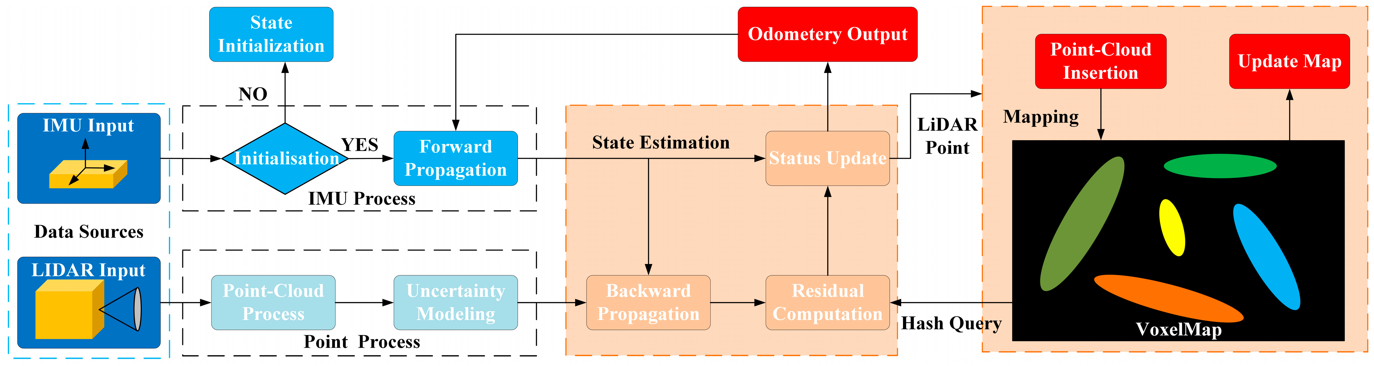
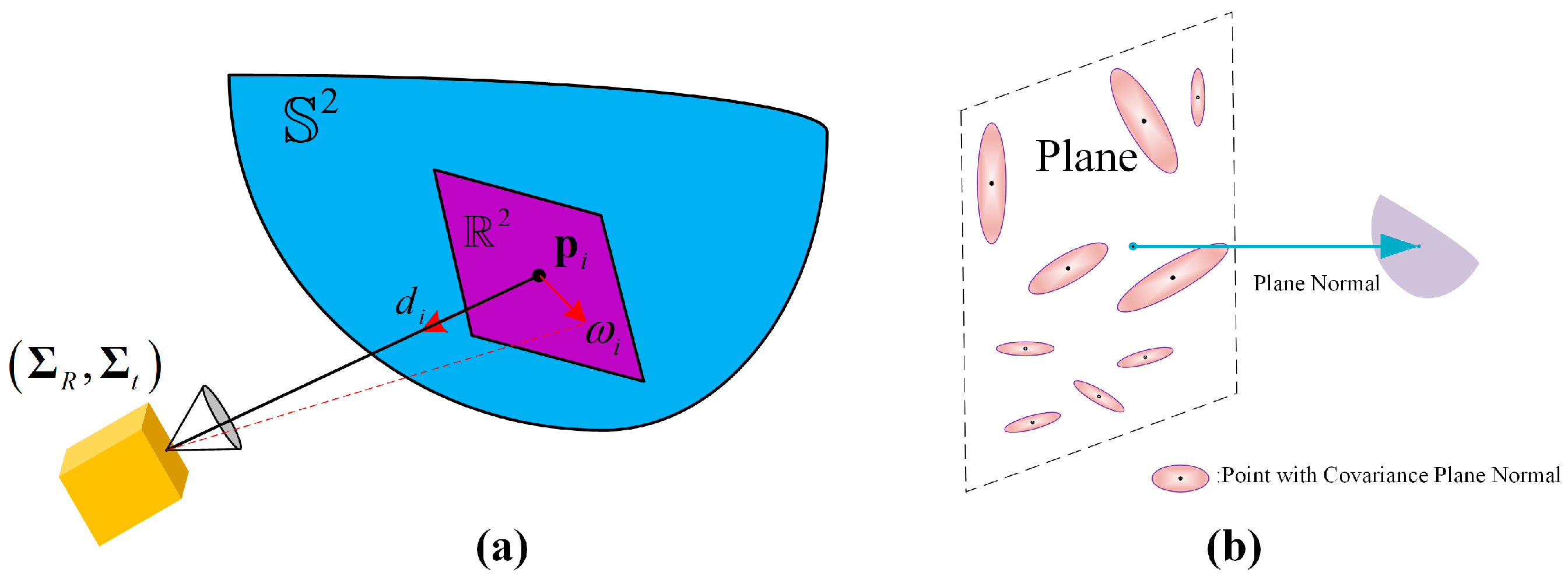
3.3. Data Process

(1)

IMU Process

A discrete-time model consistent with the continuous kinematics equations presented in [11] is formulated with respect to the state vector defined in (1):

$${\mathbf{x}}_{k+1}={\mathbf{x}}_k⊞\mathbf{f}\left({\mathit{x}}_k,{\mathit{u}}_k,{\mathit{w}}_k\right)$$

(7)

where ${\mathbf{u}}_k,{\mathbf{w}}_k$, and $\mathbf{f}$ are the system input, system noise, and kinematics function, respectively. Firstly, the mean of the nominal state ${\widehat{\mathbf{x}}}_i$ will be predicted without considering the noise ${\mathbf{w}}_k$:

$$\begin{gathered} {\widehat{\mathbf{x}}}_{k+1}={\widehat{\mathbf{x}}}_k⊞\mathbf{f}\left({\widehat{\mathbf{x}}}_k,{\mathbf{u}}_k,\mathbf{0}\right); \\ {\widehat{\mathbf{x}}}_0={\overline{\mathbf{x}}}_{k-1}. \end{gathered}$$

(8)

Consequently, this will result in the accumulation of inaccuracies. To cope with the problem, ${\mathbf{w}}_k$ is taken into account in the prediction of the error state $\delta {\mathbf{x}}_k$

$$\begin{gathered} \delta {\mathbf{x}}_{k+1}\approx {\mathbf{F}}_{\delta \mathbf{x}}\delta {\mathbf{x}}_k+{\mathbf{F}}_{\mathbf{w}}{\mathbf{w}}_k; \\ \delta {\mathbf{x}}_0=\delta {\overline{\mathbf{x}}}_{k-1}=0. \end{gathered}$$

(9)

where ${\mathbf{F}}_{\delta \mathbf{x}}$ and ${\mathbf{F}}_{\mathbf{w}}$ are the Jacobian matrices of () with respect to $\delta {\mathbf{x}}_k$ and ${\mathrm{w}}_k$. In the implementation, the system noise wi is considered as Gaussian white noise following the normal distribution $\mathcal{N}\left(\mathbf{0},\mathbf{W}\right)$, where $\mathbf{W}$ is the covariance matrix. The error state δxi is an independent random vector with a multivariate normal distribution: $\delta {\mathbf{x}}_k\sim \mathcal{N}\left(\mathbf{0},{\mathbf{P}}_k\right)$. As a consequence, the predicted covariance matrix ${\widehat{\mathbf{P}}}_{k+1}$ of $\delta {\mathbf{x}}_{k+1}$ can be calculated as the following linear transformation:

$${\widehat{\mathbf{P}}}_{k+1}={\mathbf{F}}_{\delta \mathbf{x}}{\widehat{\mathbf{P}}}_k{\mathbf{F}}_{\delta \mathbf{x}}^T+{\mathbf{F}}_{\mathbf{w}}\mathbf{W}{\mathbf{F}}_{\mathbf{w}}^T;{\widehat{\mathbf{P}}}_0={\overline{\mathbf{P}}}_{k-1}.$$

(10)

The IMU process module utilizes the state estimate from the previous scan as the initial condition and recursively predicts ${\widehat{\mathbf{x}}}_{k+1}$, $\delta {\mathbf{x}}_{k+1}$ and ${\widehat{\mathbf{P}}}_{k+1}$ till the end time of the current LiDAR scan $t_k$.

(2)

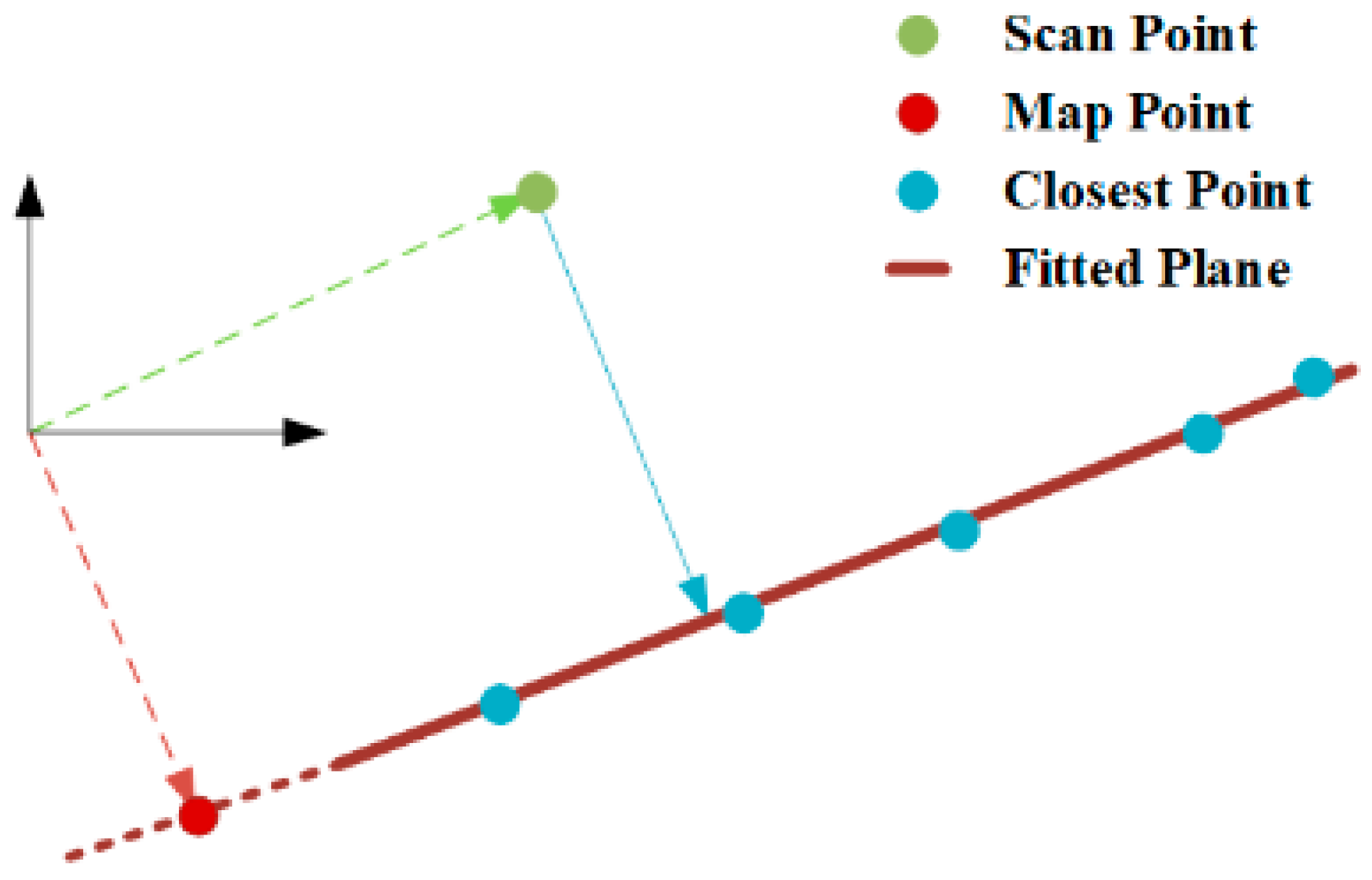
LiDAR Process

All the LiDAR points ${}^{L_j}\mathbf{p}_j$ with timestamps ${\gamma }_j\in \left[t_k-1,t_k\right]$ are cached to form a point cloud ${\mathcal{P}}_k$. In order to account for the effect of LiDAR measurement noise, each point ${}^{L_j}\mathbf{p}_j$ is accompanied by a covariance matrix ${\Sigma }_{{\mathbf{w}}_i}$, representing the measurement uncertainty. For most commercial LiDAR, the points are sampled under different timestamps, which will introduce motion distortion to the cloud ${\mathcal{P}}_k$.

To remove motion-induced distortion, every point in ${\mathcal{P}}_k$ is re-projected into the LiDAR frame $L_k$ at time $t_k$. Leveraging the backward propagation scheme proposed in [10], the relative pose ${}^{L_j}\mathbf{T}_{I_j}$ between the IMU frame at each sampling instant ${\gamma }_j$ and the LiDAR frame at $t_k$ is first recovered. Each point ${}^{L_j}\mathbf{p}_j$ is then transformed into $L_k$ by the following:

$${}^{L_k}\mathbf{p}_j={}^{I}T_{\mathrm{L}}^{-1}{}^{I_k}\mathbf{T}_{I_j}{}^{I}T_L{}^{L_j}\mathbf{p}_j$$

(11)

where ${}^I\mathbf{T}_L$ are known external parameters. The projected points ${}^{L_k}\mathbf{p}_j$ are used to construct residuals. These residuals will be used in the subsequent state estimation and point-cloud matching process, taking into account the effect of uncertainty.

3.4. Iterated State Estimation

Upon completion of the IMU and LiDAR processes, the following steps for the IESKF-based LIO system involve correspondence matching, residual formulation, and Kalman update. However, existing filter-based LIO systems [10,12,17] typically adopt the nearest correspondence matching strategy and treat the ensuing point-to-feature distance as the residual. This strategy involves projecting ${}^{L_k}\mathbf{p}_j$ to the global frame as follows:

$${}^G\widehat{\mathbf{p}}_j={}^G\widehat{\mathbf{T}}_{I_k}{}^{I}T_L{}^{L_k}\mathbf{p}_j={}^G\overline{\mathbf{T}}_{I_{k-1}}{}^{I_{k-1}}\widehat{\mathbf{T}}_{I_k}{}^{I}T_L{}^L\mathbf{p}_j$$

(12)

Long-term odometry is susceptible to positioning drift, which can introduce errors into the ${}^G\overline{\mathbf{T}}_{I_{k-1}}$ error. Additionally, spike noise in low-cost IMUs can lead to inaccuracies in ${}^{I_{k-1}}\widehat{\mathbf{T}}_{I_k}$, causing mismatches in ${}^{L_k}\mathbf{p}_j$ projections to their corresponding features. Large-scale feature association is computationally intensive. To address this, an uncertainty-aware residual model is developed for the IESKF that establishes intermediate geometric relationships, as shown in Figure 3. The formulation reduces correspondence mismatches while preserving computational efficiency; detailed derivations are provided in the following sections.

Correspondence Match: This subsection establishes the procedure for associating incoming LiDAR points with the global voxel map, thereby generating geometric constraints for attitude estimation and point-cloud alignment. Relying on the previously derived point- and plane-wise uncertainties, a point-to-plane scan-matching objective is implemented following [18]. For a LiDAR point ${\mathbf{p}}_i$ whose world-frame pose has been predicted a priori, the root voxel (coarse resolution) containing ${\mathbf{p}}_i$ is identified via its hash key. All sub-voxels within this root voxel are then queried for potential correspondences. Consider a sub-voxel hosting a planar feature characterized by normal ${\mathbf{n}}_i$ and centroid ${\mathbf{q}}_i$. The orthogonal distance from ${\mathbf{p}}_i$ to the plane is as follows (Figure 4):

$$d_i={\mathbf{n}}_i^T({\mathbf{p}}_i-{\mathbf{q}}_i)$$

(13)

Accounting for uncertainties in the normal vector ${\mathbf{n}}_i$, LiDAR point ${\mathbf{p}}_i$, and center ${\mathbf{q}}_i$, the residual equation becomes the following:

$$\begin{array}{c}{d}_i=\left({\mathit{n}}_i^{gt}⊞{\delta }_{{\mathit{n}}_i}{)}^T\left[{(}^W{\mathit{p}}_i^{gt}+{\delta }_{W_{{\mathit{p}}_i}}\right)-{\mathit{q}}_i^{gt}-{\delta }_{{\mathit{q}}_i}\right]\\ \approx {\mathbf{n}}_i^T{\mathbf{p}}_i-{\mathbf{q}}_i^T+{\mathbf{J}}_{{\mathbf{n}}_i}\delta {\mathbf{n}}_i+{\mathbf{J}}_{{\mathbf{q}}_i}\delta {\mathbf{q}}_i+{\mathbf{J}}_{{\mathbf{p}}_i}\delta {\mathbf{p}}_i\end{array}$$

(14)

which implies

$$d_i\sim \mathcal{N}\left(0,{\Sigma }_{{\mathit{w}}_i}\right),{\mathsf{\Sigma }}_{{\mathbf{w}}_i}={\mathbf{J}}_{{\mathbf{w}}_i}{\mathsf{\Sigma }}_{{\mathbf{n}}_i,{\mathbf{q}}_i,{\mathbf{p}}_i}{\mathbf{J}}_{{\mathbf{w}}_i}^T,$$

(15)

where

$$\begin{array}{c}{\mathbf{J}}_{{\mathbf{w}}_i}=\left[{\mathbf{J}}_{{\mathbf{n}}_i},{\mathbf{J}}_{{\mathbf{q}}_i},{\mathbf{J}}_{W_{{\mathbf{p}}_i}}\right]=\left[{\left({\mathbf{p}}_i-{\mathbf{q}}_i\right)}^T,-{\mathbf{n}}_i^T,{\mathbf{n}}_i^T\right]\\ {\mathsf{\Sigma }}_{{\mathbf{n}}_i,{\mathbf{q}}_i,{\mathbf{p}}_i}=\left[\begin{array}{cc}{\mathsf{\Sigma }}_{{\mathbf{n}}_i,{\mathbf{q}}_i}& 0\\ 0& {\mathsf{\Sigma }}_{{\mathbf{p}}_i}\end{array}\right]\end{array}$$

(16)

The signed distance $d_i$ follows the normal distribution $N\left(0,{\Sigma }_{{\mathbf{w}}_i}\right)$, with ${\Sigma }_{{\mathbf{w}}_i}$ denoting the covariance of the compounded uncertainties. Let ${\mathcal{V}}_j$ be the neighbour set of occupied voxels (selection illustrated in Figure 5). For every voxel ${}^G\mathbf{v}_i\left({}^G\mathbf{v}_i\in {\mathcal{V}}_j\right)$, source and target distributions are computed. If the query point lies on the candidate plane, its distance $d_i$ must conform to the stated distribution. With the distribution’s standard deviation set to $\sigma =\sqrt{{\Sigma }_{{\mathbf{w}}_i}}$, a point is retained as a valid correspondence when its measured distance satisfies $3\sigma$. Should no plane satisfy this criterion, the point is discarded to suppress potential false matches.

Residual Formulation: Prior to introducing the novel residual metric, it is imperative to elucidate the observation model and state estimation framework employed within the IESKF. This clarification will underpin the rationale for the proposed residual metric. The observation function of the system is as follows:

$${\mathbf{z}}_k^n=\mathbf{h}\left({\widehat{\mathbf{x}}}_k^n⊞\delta {\mathbf{x}}_k^n\right)+{\mathbf{v}}_k,$$

(17)

where ${\mathbf{v}}_k$ represents the measurement noise, which is normally distributed as ${\mathbf{v}}_k\sim n(0,{\mathbf{V}}_k)$, and $\mathbf{h}$() denotes the observation function that projects the state space onto the observation space. Given the small magnitude of the error state, the observation function is linearized about the estimate ${\widehat{\mathbf{x}}}_k^n$:

$${\mathbf{z}}_k^n\approx \mathbf{h}\left({\widehat{\mathbf{x}}}_k^n\right)+{\mathbf{H}}^n\delta {\mathbf{x}}_k^n+{\mathbf{v}}_k,$$

(18)

where the Jacobian matrix ${\mathbf{H}}^n$ is defined as the derivative of $\mathbf{h}\left({\widehat{\mathbf{x}}}_k^n⊞\delta {\mathbf{x}}_k^n\right)$ with respect to $\delta {\mathbf{x}}_k^n$. Since $\delta {\mathbf{x}}_k$ and $\delta {\mathbf{x}}_k^n$ reside in different tangent spaces of the manifold $\mathcal{M}$ (the tangent spaces of ${\widehat{\mathbf{x}}}_k$ and ${\widehat{\mathbf{x}}}_k^n$, respectively), the error state $\delta {\mathbf{x}}_k$ is projected onto $\delta {\widehat{\mathbf{x}}}_k^n$ via the following:

$$\delta {\mathbf{x}}_k=\left({\widehat{\mathbf{x}}}_k^n⊞\delta {\mathbf{x}}_k^n\right)\boxminus {\widehat{\mathbf{x}}}_k={\widehat{\mathbf{x}}}_k^n⊞{\widehat{\mathbf{x}}}_k+{\left({\mathbf{J}}^n\right)}^{-1}\delta {\mathbf{x}}_k^n,$$

(19)

where ${\mathbf{J}}^n$ is the inverse of the Jacobian matrix of $\left({\widehat{\mathbf{x}}}_k^n⊞\delta {\mathbf{x}}_k^n\right)\boxminus {\widehat{\mathbf{x}}}_k$ with respect to ${\mathbf{x}}_k^n$. Incorporating Equations (18) and (19) within the Bayesian framework yields the maximum a posteriori (MAP) estimation problem:

$$\delta {\mathbf{x}}_k^n=arg\underset{\delta {\mathbf{x}}_k^n}{\mathrm{m}\mathrm{i}\mathrm{n}}\left({\parallel \delta {\mathbf{x}}_k\parallel }_{{\widehat{\mathbf{P}}}_k^{-1}}^2+{\parallel \mathbf{h}\left({\widehat{\mathbf{x}}}_k^n\right)+{\mathbf{H}}^n\delta {\mathbf{x}}_k^n\parallel }_{{\mathbf{V}}_k^{-1}}^2\right)$$

(20)

State update: Combining the prior distribution of $\mathbf{x}$ with the measurement model generates the posterior distribution of state ${\mathbf{x}}_k$, equivalently represented as ${\tilde{\mathbf{x}}}_k^{\kappa }$ and its maximum a posteriori (MAP) estimate. This prior will be fused with the point-to-plane distance matched to form a maximum a posteriori (MAP) estimation. Combining the state a priori with all valid measurements gives us the MAP estimate:

$$\delta \underset{{\mathbf{x}}_k}{min}\left({\parallel {\mathbf{x}}_k⊞{\widehat{\mathbf{x}}}_k\parallel }_{{\widehat{\mathbf{P}}}_k^{-1}}^2+\sum _{i=1}^m{\parallel d_i-{\mathbf{H}}_i\cdot \left({\mathbf{x}}_k⊞{\overline{\mathbf{x}}}_k\right)\parallel }_{{\mathbf{V}}_k^{-1}}^2\right)$$

(21)

where there are ${\parallel \mathbf{x}\parallel }_{\mathbf{M}}^2={\mathbf{x}}^T{\mathbf{M}}^{-1}\mathbf{x}$, and $m$ is the total number of valid feature points in the $k$-th frame.

3.5. Incremental Global Map

SS-LIO employs surfels as the underlying map representation to support efficient fusion of incoming LiDAR points and incremental map updates. The environment is partitioned into voxels of fixed resolution—one meter on each side—and every voxel stores the set of points that jointly define a surfel, following the structure introduced in reference [18]. Each voxel index is computed from its three-dimensional coordinates by a dedicated hash function and stored in an unordered map, guaranteeing constant-time surfel–point associations.

Map Construction: The voxel map characterizes each voxel $\mathcal{M}\left[i\right]$ by five elements: the number of points N, the sum of points p, the sum of outer products C, the mean of voxel μ, and the covariance of voxel Σ. The hash index is calculated as follows:

$$\begin{array}{c}go=⌊{\displaystyle \frac{p_z}{s}}⌋\times n_z\times n_y\times n_z+⌊{\displaystyle \frac{p_y}{s}}⌋\times n_z+⌊{\displaystyle \frac{p_z}{s}}⌋\\ hashindex=go\hspace{0.33em}mod{M}_{max}\end{array}$$

(22)

where $p_x,p_y$, and $p_z$ are the position of the laser point $p\in {\mathbb{R}}^3$. The function $\lfloor x\rfloor$ calculates the maximum integer value that is not greater than $x$. The parameter $s$ is the voxel resolution and $M_{\mathrm{m}\mathrm{a}\mathrm{x}}$ is the maximum size in the voxel map. The values $n_x,n_y$, and $n_z$ are the number of large voxels.

The voxel map increment consists of two steps: update and delete. For the update step, the undistorted scan ${\mathcal{P}}_k$ is transformed into the world frame by a posteriori estimation ${\widehat{\mathbf{x}}}_k$. The laser points in ${\mathcal{P}}_k$ are subsequently stored in the active list $\mathcal{V}$ according to the hash index in (22). For each hash index in the active list $\mathcal{V}$, the number of laser points ${\tilde{N}}_i$, the sum of the points $\tilde{\mathbf{p}}$, and the sum of the outer products ${\tilde{\mathbf{C}}}_i$ are computed to update the voxel $\mathcal{M}\left[i\right]$:

$$\begin{array}{c}\begin{array}{c}\mathcal{M}\left[i\right].N=\mathcal{M}\left[i\right].N+N_i\\ \mathcal{M}\left[i\right].p=\mathcal{M}\left[i\right].p+p_i\end{array}\\ \begin{array}{c}\begin{array}{c}\mathcal{M}\left[i\right].C=\mathcal{M}\left[i\right].C+C_i\\ \mathcal{M}\left[i\right].\mu ={\displaystyle \frac{\mathcal{M}\left[i\right].p}{\mathcal{M}\left[i\right].N}}\end{array}\\ \mathcal{M}\left[i\right].\mathsf{\Sigma }={\displaystyle \frac{1}{\mathcal{M}\left[i\right].N+1}}\left(\mathcal{M}\left[i\right].C-\mathcal{M}\left[i\right].p\cdot \mathcal{M}\left[i\right].{\mu }^T\right)\end{array}\end{array}$$

(23)

The purpose of the deletion step is to strike a balance between the storage space of the voxel map and the accuracy of the alignment.

4. Experimental Results and Analysis

4.1. Experimental Setup

In this section, the performance of the proposed system is assessed for accuracy and time efficiency. The experiments were conducted on a computer with an i7-12700H processor and 16 GB of RAM, encompassing validation on both public and private datasets. To ascertain the methodology’s validity and precision, SS-LIO was benchmarked against leading LIO systems: FAST-LIO2, POINT-LIO, LOAM-LIVOX [26], and SI-LIO, utilizing their default open-source parameters for evaluations in both indoor and outdoor settings. The outcomes of these experiments, which are reported as the mean of five experiments, substantiate our methodological exposition.

(i)

The system exhibits estimation accuracy on par with cutting-edge LIO systems.

(ii)

It delivers precise pose estimation across diverse environments and motion profiles.

(iii)

It achieves superior localization and mapping in indoor environments with degraded conditions.

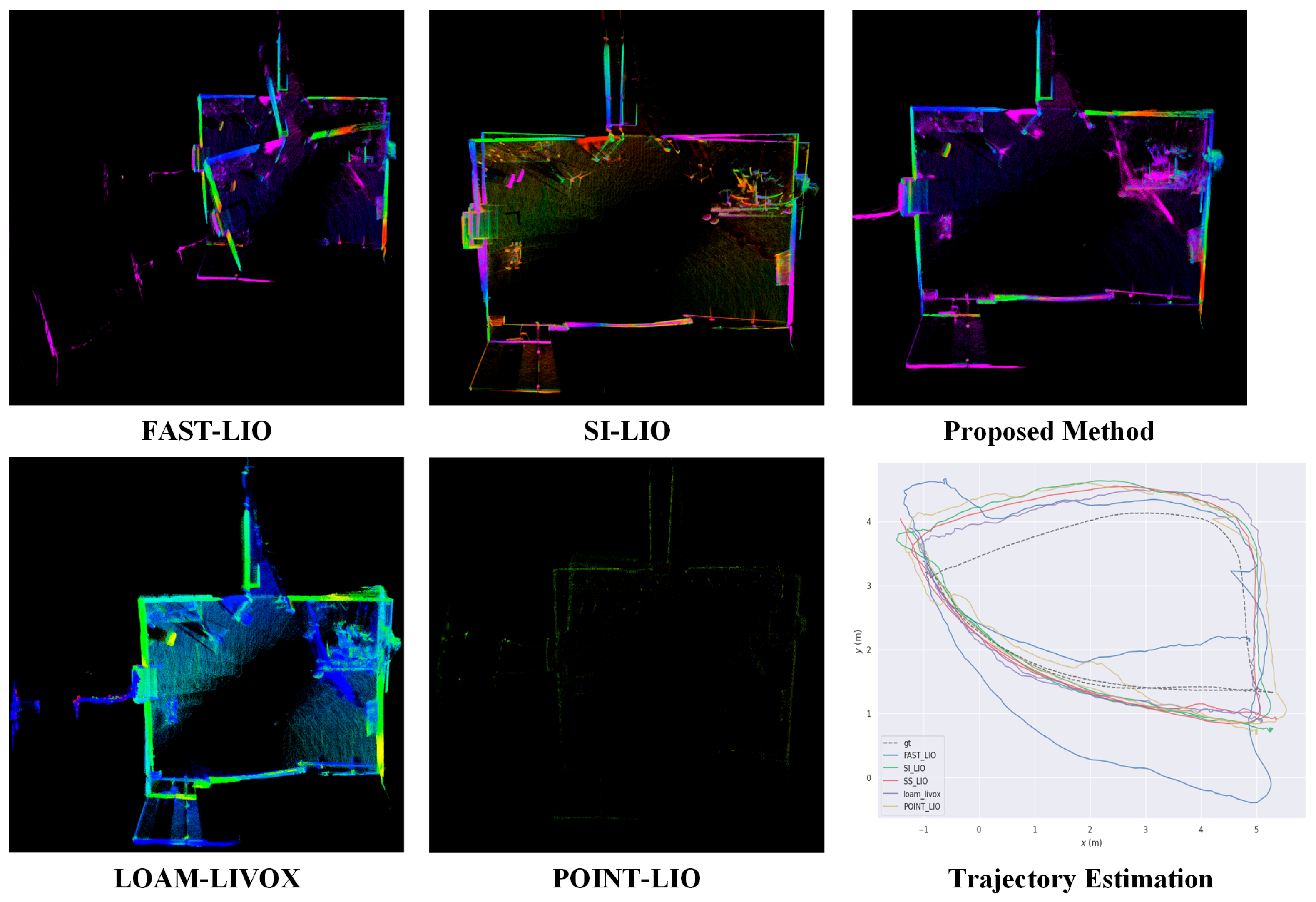
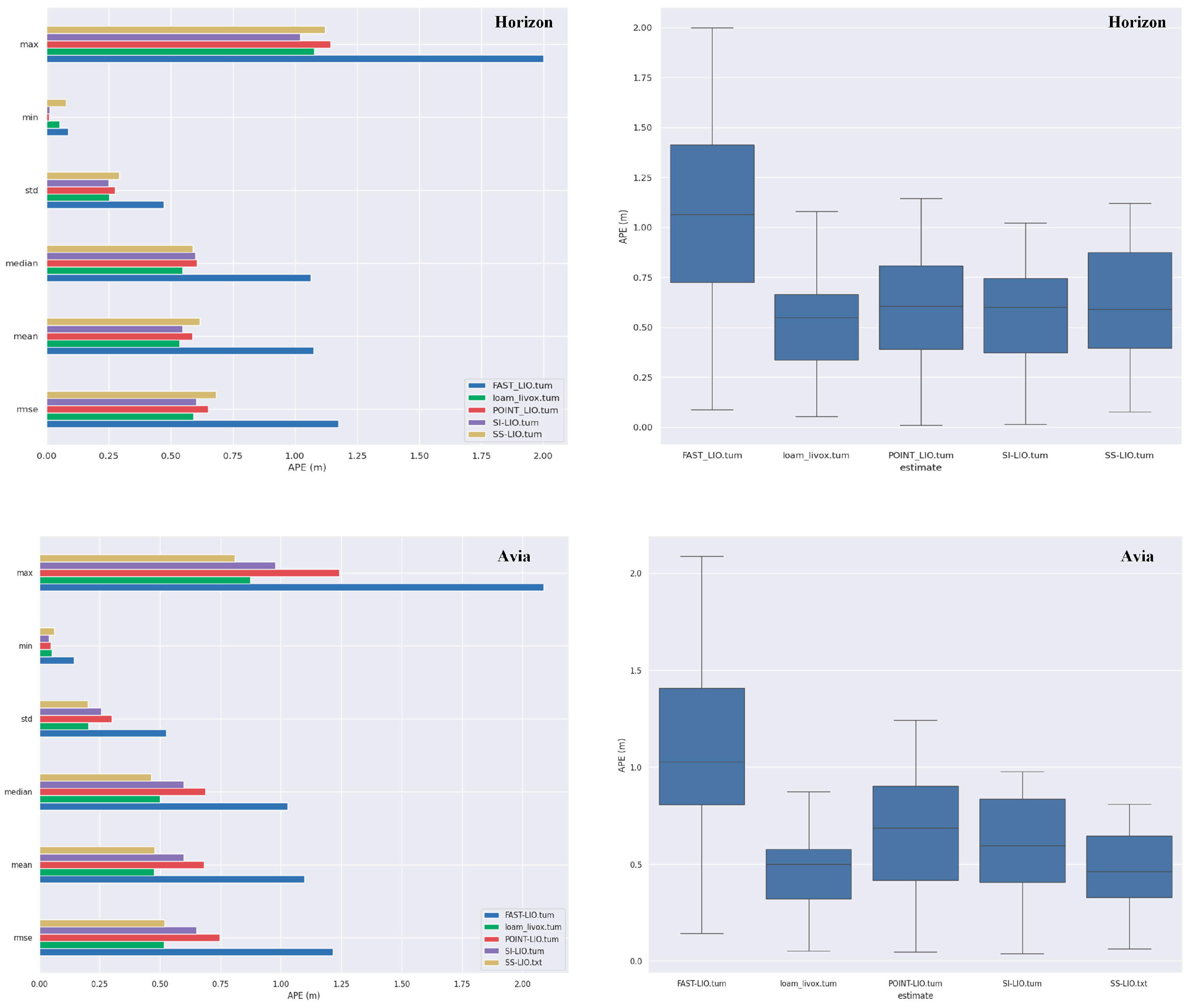
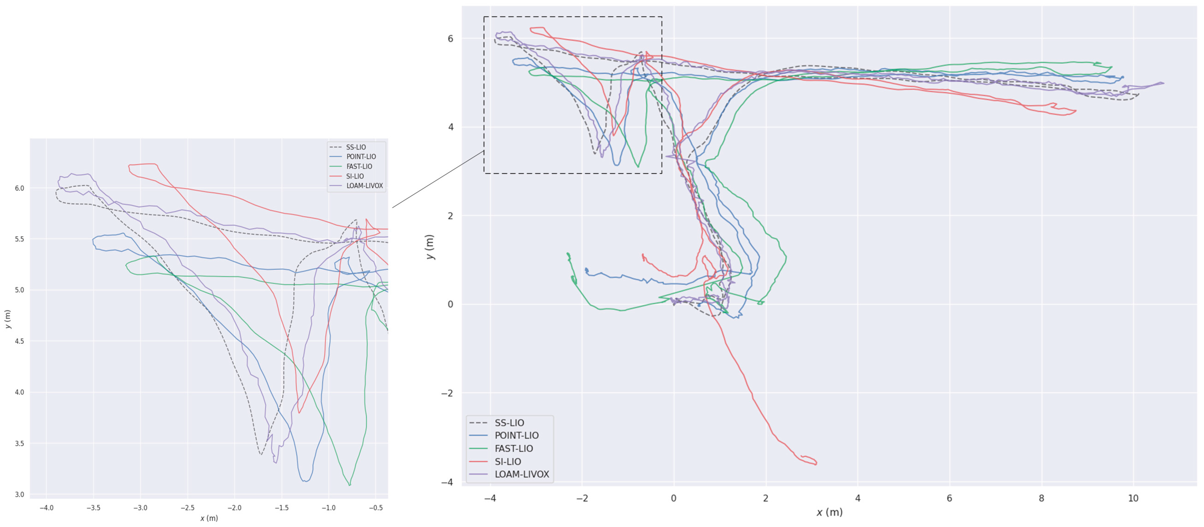
4.2. Evaluation of Odometry Accuracy

(1)

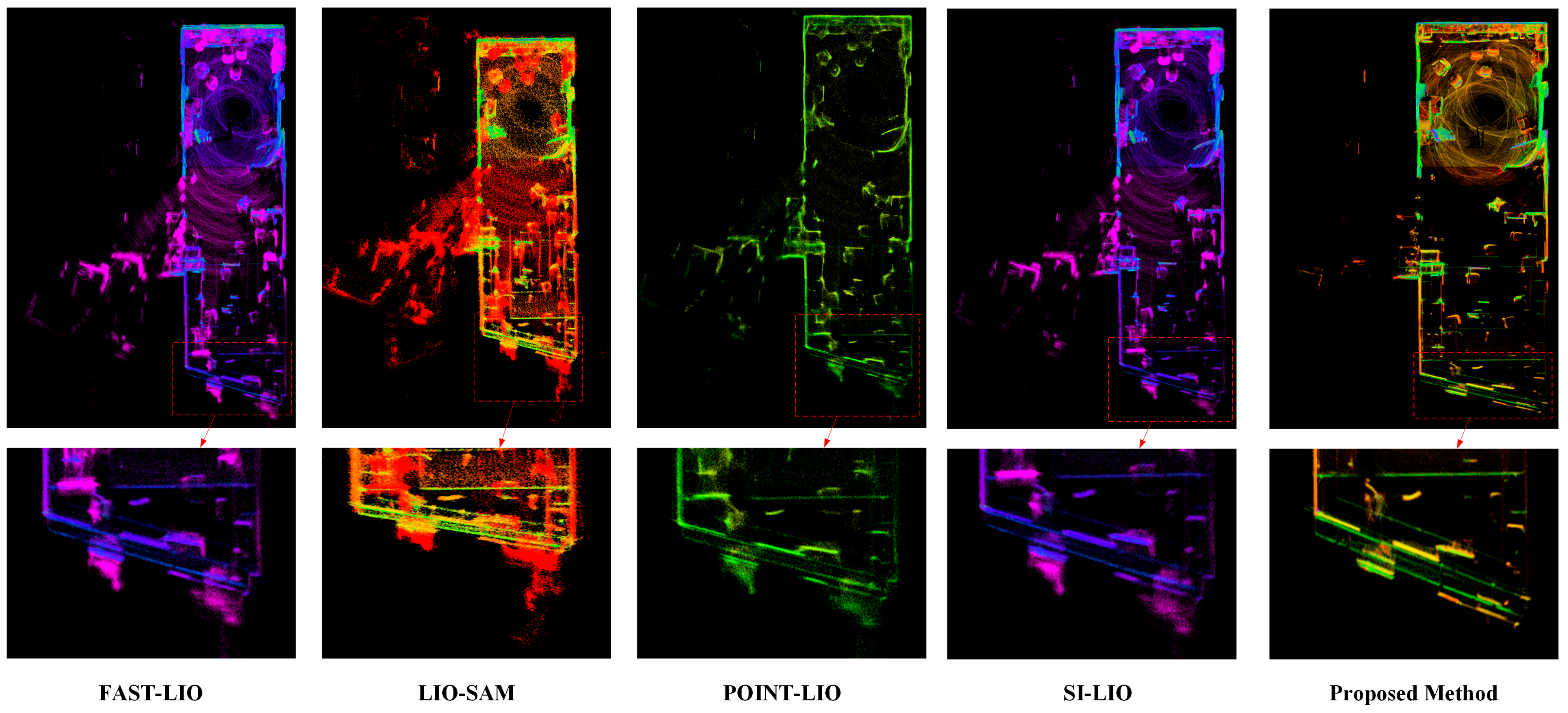
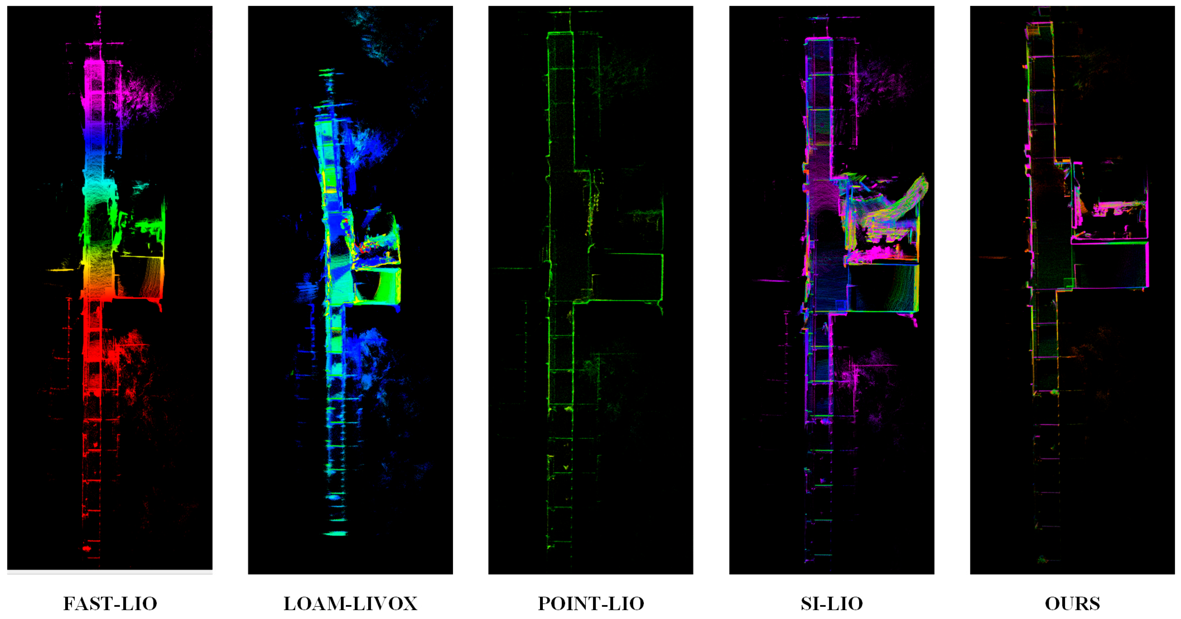
LiDAR degeneration experiment: Evaluation is conducted on the indoor degenerate sequence degenerate_seq_02 from the R3LIVE dataset [27] and the indoor split of the LiDAR_Degenerated dataset [28], both recorded with a Livox Avia operating at 10 Hz and offering a 70.4° × 77.2° non-repetitive field of view. These sequences highlight the geometric weakness inherent to solid-state LiDAR in corridor-like environments. To broaden the scope, indoor02 and indoor03 from the Tiers-LiDAR [29] dataset are included, providing time-synchronized measurements from the same Avia and a Livox Horizon running at 10 Hz with an 81.7° × 25.1° field of view. The Horizon’s wider horizontal but substantially narrower vertical coverage delivers complementary geometric constraints, enabling a controlled assessment of degeneracy effects across two distinct solid-state LiDAR configurations.

For the indoor degradation scenario represented by degenerate_seq_02, Figure 6 illustrates the mapping outcomes of the four approaches. Our method exhibits enhanced robustness and precision relative to the other three. Specifically, our SS-LIO method, which incorporates an uncertainty model, effectively manages the challenges of degraded environments. Compared to FAST-LIO2, our system achieves a minimum end-to-end drift of 0.2 m, outperforming the SI-LIO method that also uses voxels. This indicates that in indoor degraded settings, our method not only demonstrates robustness but also yields more precise localization and mapping outcomes.

In the degraded scene of the LiDAR_Degenerated indoor dataset, which features a wall approximately 30 m in length, Figure 7 shows that SS-LIO successfully navigates back to the starting point. The two regions, nearly coplanar with the wall, lead to erroneous attitude estimation for FAST-LIO2, preventing it from returning to the starting position. SI-LIO, lacking the integration of an uncertainty model in pose estimation, also fails to return to the starting point. Compared to FAST-LIO2 and SI-LIO, our system demonstrates greater robustness and accuracy in these scenarios, achieving an accuracy level comparable to that of FAST-LIVO.

Comprehensive evaluation on the Tiers-LiDAR indoor sequences—specifically illustrated in Figure 8, Figure 9 and Figure 10—establishes SS-LIO as superior in trajectory accuracy, map fidelity and robustness. In indoor02, the trajectory yields a root-mean-square error of 0.61 m, and the corresponding map exhibits sharply delineated edges, uniform wall thickness, and negligible ghosting. Analysis of the error distribution reveals a median absolute pose error of 0.25 m—half that of SI-LIO at 0.50 m—while all errors remain below 0.50 m; FAST-LIO and POINT-LIO exhibit drift exceeding 1.20 m with pronounced heavy-tailed distributions. In the more challenging indoor03, SS-LIO maintains crisp boundaries and wall parallelism, whereas POINT-LIO and SI-LIO manifest inter-layer misalignment and phantom walls, LOAM-LIVOX drifts along the corridor axis, and FAST-LIO fails under repetitive structures and aggressive motion. Overall, localization accuracy improves by 10% relative to SI-LIO and 83% relative to FAST-LIO, while a structurally coherent high-fidelity map is consistently generated, confirming the synergistic efficacy of surfel-based uncertainty modeling coupled with IESKF residual design in preserving state estimation precision and map integrity within complex indoor environments.

(2)

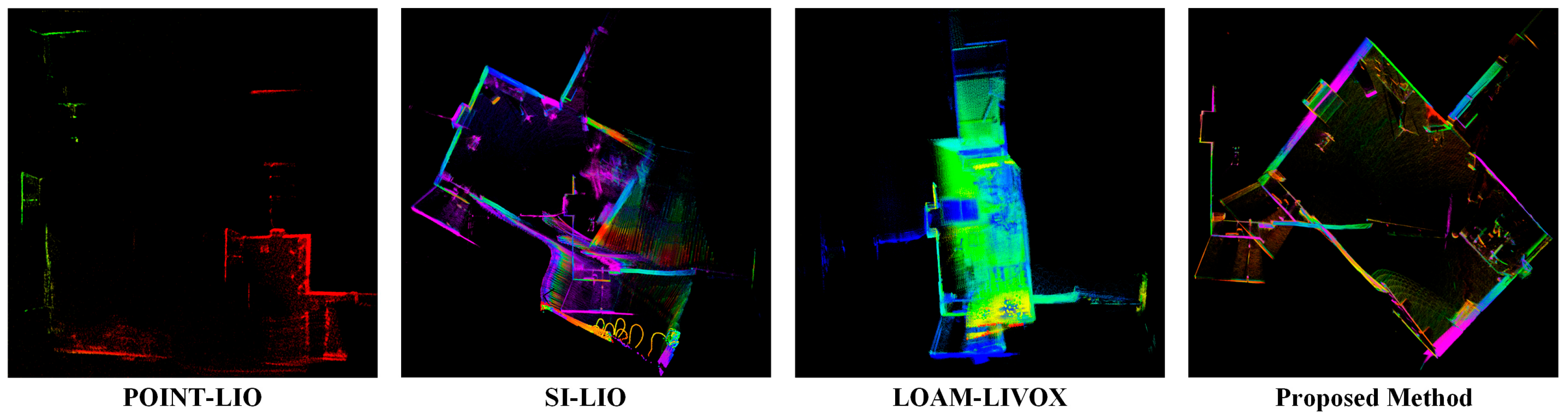
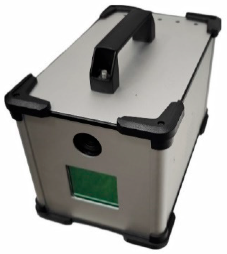
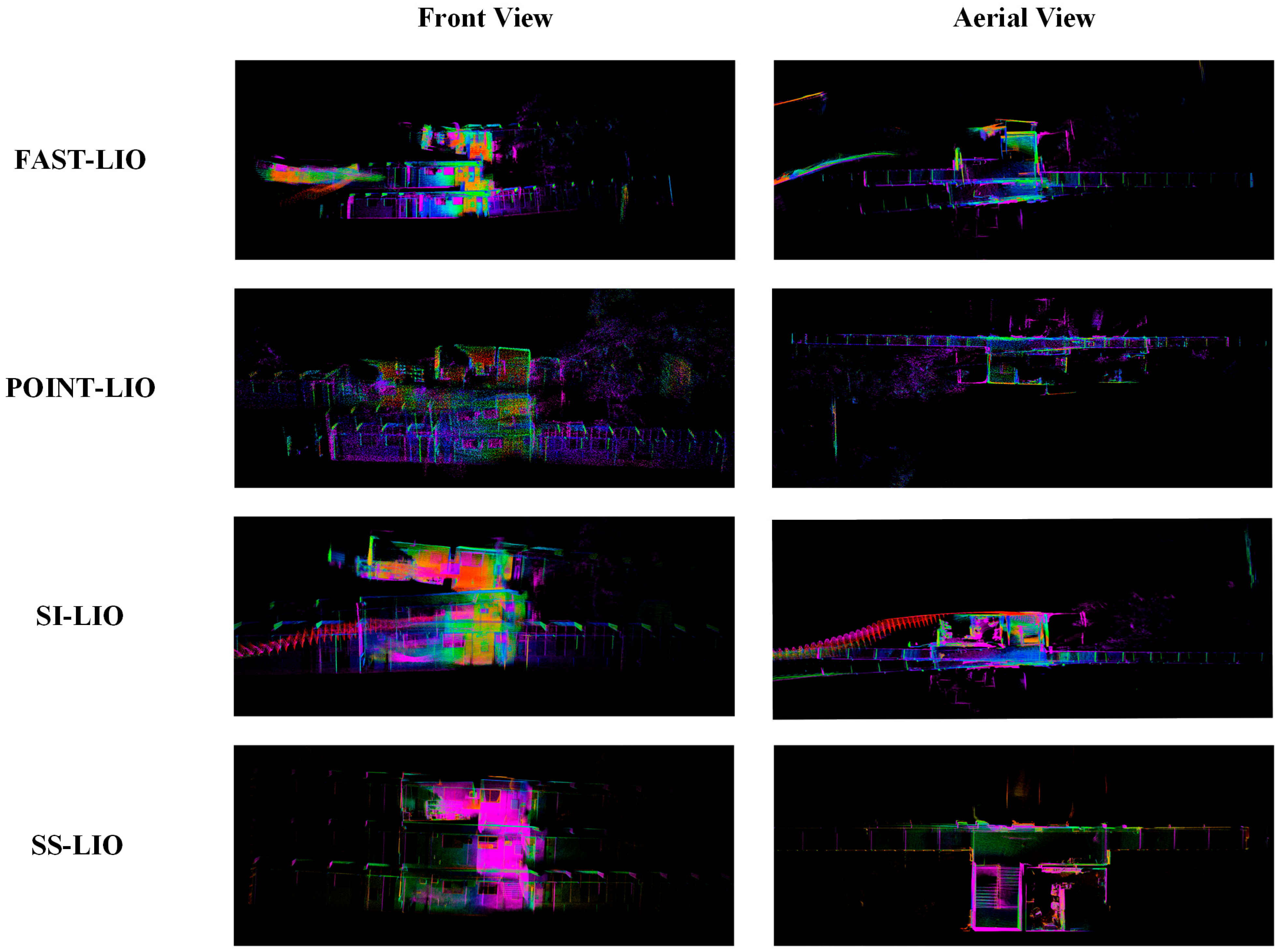
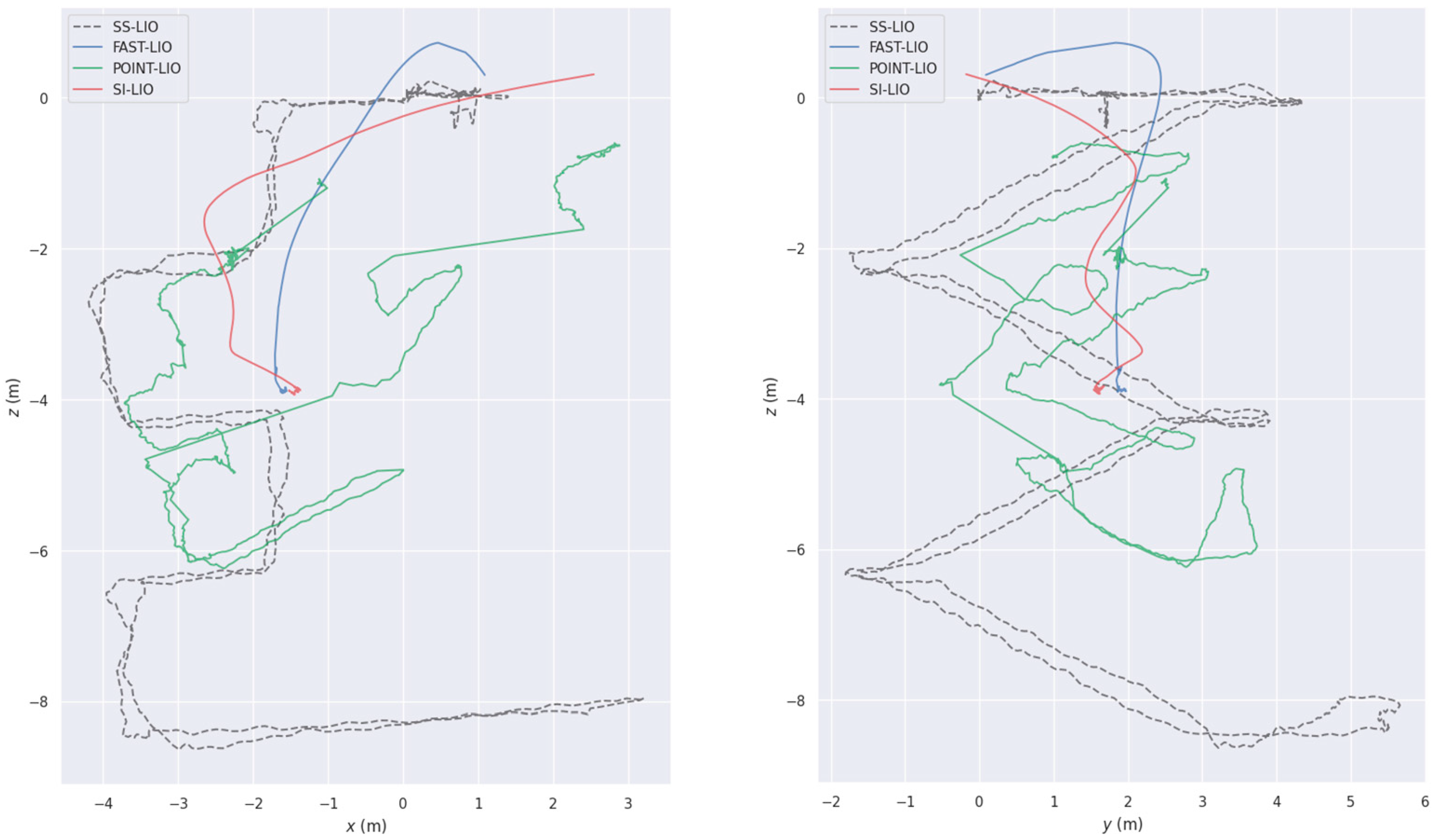
Private Dataset: The SS-LIO system is evaluated on two purposely collected indoor sequences—a geometrically degraded long corridor and a corridor with integrated stairs—engineered to rigorously test localization stability and mapping accuracy under demanding conditions. Figure 11 shows the photos of our data collection equipment.

As shown in Figure 12 and Figure 13, the proposed SS-LIO system demonstrates significant advantages in single-layer LiDAR mapping in single-layer long corridor degraded environments. SS-LIO employs voxel modeling, which provides a more refined spatial representation and effectively captures the environmental complexity. This approach enhances the system’s sensitivity to environmental features, thereby improving its robustness and stability in position estimation, which is crucial for long-term localization. In contrast, FAST-LIO2, which relies on ikd-Tree methods, often experiences trajectory drift, and requires parameter adjustments that yield suboptimal outcomes. SI-LIO, on the other hand, exhibits instability in z-axis estimation and fails to provide a stable estimation. Additionally, LOAM-LIVOX, while effective in certain scenarios, shows limitations in maintaining consistent and detailed maps in single-layer long corridor degraded environments.

The proposed SS-LIO system exhibits remarkable performance in multi-story degraded environments, as shown in Figure 14 and Figure 15. In these challenging scenarios, our method produces a more detailed and accurate point-cloud map compared to FAST-LIO, POINT-LIO, and SI-LIO. The trajectory estimation from SS-LIO is smoother and more precise, with less drift and deviation. LOAM-LIVOX, however, struggles to generate a reliable map and provide accurate localization in this environment. The point-cloud map from LOAM-LIVOX is sparse and incomplete, and its trajectory estimation is highly unstable. This clearly demonstrates the proposed method’s advantages in multi-story degraded scenarios, making it more reliable and effective for LiDAR localization and mapping tasks.

The experimental results clearly indicate that SS-LIO outperforms FAST-LIO2, SI-LIO, and LOAM-LIVOX in these degraded environments, maintaining more accurate and reliable mapping outcomes. The voxel construction in SS-LIO not only improves the precision of the map but also ensures that the system can handle the lack of geometric features and edge information more effectively, making it a superior choice for LiDAR mapping in complex indoor settings.

5. Conclusions

In this paper, SS-LIO is presented as a filter-based LiDAR–Inertial odometry framework designed for solid-state LiDAR operating in geometrically degraded indoor environments. Points are modeled as uncertain entities to enable robust correspondence establishment. A voxel-centric residual metric replaces the conventional point-to-plane distance, yielding improved estimation accuracy and streamlined map maintenance. Extensive evaluations on multiple datasets confirm that SS-LIO outperforms state-of-the-art methods in pose accuracy and map consistency. The integration of voxel techniques with probabilistic point modeling markedly increases robustness under severe LiDAR degradation. Future efforts will focus on parallelizing voxel mapping and refining the filter structure to reduce computational latency.

References

- Qin, T.; Li, P.; Shen, S. VINS-Mono: A Robust and Versatile Monocular Visual-Inertial State Estimator. IEEE Trans. Robot. 2018, 34, 1004–1020. [Google Scholar] [CrossRef]
- Sun, K.; Mohta, K.; Pfrommer, B.; Watterson, M.; Liu, S.; Mulgaonkar, Y.; Taylor, C.J.; Kumar, V. Robust Stereo Visual Inertial Odometry for Fast Autonomous Flight. IEEE Robot. Autom. Lett. 2018, 3, 965–972. [Google Scholar] [CrossRef]
- Campos, C.; Elvira, R.; Rodríguez, J.J.G.; Montiel, J.M.M.; Tardós, J.D. ORB-SLAM3: An Accurate Open-Source Library for Visual, Visual–Inertial, and Multimap SLAM. IEEE Trans. Robot. 2021, 37, 1874–1890. [Google Scholar] [CrossRef]
- Bloesch, M.; Czarnowski, J.; Clark, R.; Leutenegger, S.; Davison, A.J. CodeSLAM-Learning a Compact, Optimisable Representation for Dense Visual SLAM. In Proceedings of the 2018 IEEE/CVF Conference on Computer Vision and Pattern Recognition, Salt Lake City, UT, USA, 18–23 June 2018; pp. 2560–2568. [Google Scholar]
- Dellenbach, P.; Deschaud, J.-E.; Jacquet, B.; Goulette, F. CT-ICP: Real-Time Elastic LiDAR Odometry with Loop Closure. In Proceedings of the 2022 International Conference on Robotics and Automation (ICRA), Philadelphia, PA, USA, 23–27 May 2022; pp. 5580–5586. [Google Scholar]
- Chen, K.; Lopez, B.T.; Agha-mohammadi, A.; Mehta, A. Direct LiDAR Odometry: Fast Localization With Dense Point Clouds. IEEE Robot. Autom. Lett. 2022, 7, 2000–2007. [Google Scholar] [CrossRef]
- Vizzo, I.; Guadagnino, T.; Mersch, B.; Wiesmann, L.; Behley, J.; Stachniss, C. KISS-ICP: In Defense of Point-to-Point ICP–Simple, Accurate, and Robust Registration If Done the Right Way. IEEE Robot. Autom. Lett. 2023, 8, 1029–1036. [Google Scholar] [CrossRef]
- Shan, T.; Englot, B.; Meyers, D.; Wang, W.; Ratti, C.; Rus, D. LIO-SAM: Tightly-Coupled Lidar Inertial Odometry via Smoothing and Mapping. In Proceedings of the 2020 IEEE/RSJ International Conference on Intelligent Robots and Systems (IROS), Las Vegas, NV, USA, 25–29 October 2020; pp. 5135–5142. [Google Scholar]
- Shan, T.; Englot, B. LeGO-LOAM: Lightweight and Ground-Optimized Lidar Odometry and Mapping on Variable Terrain. In Proceedings of the 2018 IEEE/RSJ International Conference on Intelligent Robots and Systems (IROS), Madrid, Spain, 1–5 October 2018; pp. 4758–4765. [Google Scholar]
- Xu, W.; Zhang, F. FAST-LIO: A Fast, Robust LiDAR–Inertial Odometry Package by Tightly-Coupled Iterated Kalman Filter. IEEE Robot. Autom. Lett. 2021, 6, 3317–3324. [Google Scholar] [CrossRef]
- Xu, W.; Cai, Y.; He, D.; Lin, J.; Zhang, F. FAST-LIO2: Fast Direct LiDAR–Inertial Odometry. IEEE Trans. Robot. 2022, 38, 2053–2073. [Google Scholar] [CrossRef]
- Bai, C.; Xiao, T.; Chen, Y.; Wang, H.; Zhang, F.; Gao, X. Faster-LIO: Lightweight Tightly Coupled LiDAR–Inertial Odometry Using Parallel Sparse Incremental Voxels. IEEE Robot. Autom. Lett. 2022, 7, 4861–4868. [Google Scholar] [CrossRef]
- Lim, H.; Kim, D.; Kim, B.; Myung, H. AdaLIO: Robust Adaptive LiDAR–Inertial Odometry in Degenerate Indoor Environments. In Proceedings of the 2023 20th International Conference on Ubiquitous Robots (UR), Honolulu, HI, USA, 25–28 June 2023; pp. 48–53. [Google Scholar]
- He, D.; Xu, W.; Chen, N.; Kong, F.; Yuan, C.; Zhang, F. Point-LIO: Robust High-Bandwidth Light Detection and Ranging Inertial Odometry. Adv. Intell. Syst. 2023, 5, 2200459. [Google Scholar] [CrossRef]
- Zhang, J.; Singh, S. LOAM: Lidar Odometry and Mapping in Real-Time. In Proceedings of the Robotics: Science and Systems, Berkeley, CA, USA, 12–16 July 2014. [Google Scholar]
- Wang, H.; Wang, C.; Chen, C.-L.; Xie, L. F-LOAM: Fast LiDAR Odometry and Mapping. In Proceedings of the 2021 IEEE/RSJ International Conference on Intelligent Robots and Systems (IROS), Prague, Czech Republic, 27 September–1 October 2021; pp. 4390–4396. [Google Scholar]
- Qin, C.; Ye, H.; Pranata, C.E.; Han, J.; Zhang, S.; Liu, M. LINS: A LiDAR–Inertial State Estimator for Robust and Efficient Navigation. In Proceedings of the 2020 IEEE International Conference on Robotics and Automation (ICRA), Paris, France, 31 May–31 August 2020; pp. 8899–8906. [Google Scholar]
- Yuan, C.; Xu, W.; Liu, X.; Hong, X.; Zhang, F. Efficient and Probabilistic Adaptive Voxel Mapping for Accurate Online LiDAR Odometry. IEEE Robot. Autom. Lett. 2022, 7, 8518–8525. [Google Scholar] [CrossRef]
- Park, C.; Moghadam, P.; Williams, J.L.; Kim, S.; Sridharan, S.; Fookes, C. Elasticity Meets Continuous-Time: Map-Centric Dense 3D LiDAR SLAM. IEEE Trans. Robot. 2022, 38, 978–997. [Google Scholar] [CrossRef]
- Nguyen, T.-M.; Duberg, D.; Jensfelt, P.; Yuan, S.; Xie, L. SLICT: Multi-Input Multi-Scale Surfel-Based LiDAR–Inertial Continuous-Time Odometry and Mapping. IEEE Robot. Autom. Lett. 2023, 8, 2102–2109. [Google Scholar] [CrossRef]
- Li, K.; Li, M.; Hanebeck, U.D. Towards High-Performance Solid-State-LiDAR–Inertial Odometry and Mapping. IEEE Robot. Autom. Lett. 2021, 6, 5167–5174. [Google Scholar] [CrossRef]
- Liu, Z.; Zhang, F. BALM: Bundle Adjustment for Lidar Mapping. IEEE Robot. Autom. Lett. 2021, 6, 3184–3191. [Google Scholar] [CrossRef]
- Zhang, C.; Zhang, J.; Liu, Q.; Liu, Y.; Qin, J. SI-LIO: High-Precision Tightly-Coupled LiDAR- Inertial Odometry via Single-Iteration Invariant Extended Kalman Filter. IEEE Robot. Autom. Lett. 2025, 10, 564–571. [Google Scholar] [CrossRef]
- Hertzberg, C.; Wagner, R.; Frese, U.; Schröder, L. Integrating Generic Sensor Fusion Algorithms with Sound State Representations through Encapsulation of Manifolds. Inf. Fusion 2013, 14, 57–77. [Google Scholar] [CrossRef]
- Ji, X.; Yuan, S.; Yin, P.; Xie, L. LIO-GVM: An Accurate, Tightly-Coupled LiDAR–Inertial Odometry With Gaussian Voxel Map. IEEE Robot. Autom. Lett. 2024, 9, 2200–2207. [Google Scholar] [CrossRef]
- Lin, J.; Zhang, F. Loam Livox: A Fast, Robust, High-Precision LiDAR Odometry and Mapping Package for LiDARs of Small FoV. In Proceedings of the 2020 IEEE International Conference on Robotics and Automation (ICRA), Paris, France, 31 May–31 August 2020; pp. 3126–3131. [Google Scholar]
- Lin, J.; Zhang, F. R3LIVE: A Robust, Real-Time, RGB-Colored, LiDAR–Inertial-Visual Tightly-Coupled State Estimation and Mapping Package. In Proceedings of the 2022 International Conference on Robotics and Automation (ICRA), Philadelphia, PA, USA, 23–27 May 2022; pp. 10672–10678. [Google Scholar]
- Zheng, C.; Zhu, Q.; Xu, W.; Liu, X.; Guo, Q.; Zhang, F. FAST-LIVO: Fast and Tightly-Coupled Sparse-Direct LiDAR–Inertial-Visual Odometry. In Proceedings of the 2022 IEEE/RSJ International Conference on Intelligent Robots and Systems (IROS), Kyoto, Japan, 23–27 October 2022; pp. 4003–4009. [Google Scholar]
- Li, Q.; Yu, X.; Queralta, J.P.; Westerlund, T. Multi-Modal Lidar Dataset for Benchmarking General-Purpose Localization and Mapping Algorithms. In Proceedings of the 2022 IEEE/RSJ International Conference on Intelligent Robots and Systems (IROS), Kyoto, Japan, 23–27 October 2022; pp. 3837–3844. [Google Scholar]