A Three-Layer Sequential Model Predictive Current Control for NNPC Four-Level Inverters with Low Common-Mode Voltage

Abstract

The four-level nested neutral point clamped (4L-NNPC) inverter has recently become a promising solution for renewable energy generation, e.g., wind and photovoltaic power. The NNPC inverter can stabilize the flying capacitor (FC) voltages of each bridge through redundant switch states (RSSs). This paper presents an improved three-layer sequential model predictive control (3LS-MPC) method for 4L-NNPCs. This method eliminates weighting factors and removes the switch states that generate high common-mode voltage (CMV). Before selecting the optimal vector, we disable certain switch states which affect the FC voltages, continuing to deviate from the desired value. Then, adopting a two-stage optimal vector selection method, we select the optimal sector based on six specific vectors and choose the optimal vector from the seven vectors in the optimal sector. The feasibility of this method was verified in Matlab/Simulink and the prototype. The experimental results show that compared with classical FCS-MPC, the proposed 3LS-MPC method reduces the common-mode voltage and has better harmonic quality and more stable FCs voltages.

1. Introduction

Nowadays, people’s attention to high-power converters is constantly increasing with the continuous development of clean energy technologies such as wind and photovoltaic power [1,2]. Multilevel inverters, as widely used power converters, have become a research hotspot in recent years. Multilevel inverters are mainly divided into neutral point clamped (NPC), flying capacitor (FC), cascaded H-bridge (CHB), and modular multilevel converter (MMC) types [3,4]. Compared with two-level inverters, they have the advantages of low harmonic content in output current and voltage, withstanding a high voltage level, high cost-effectiveness, and low dv/dt. They are mostly used in variable-speed wind energy conversion systems as part of power converters [5,6]. Compared with three-level inverters, four-level inverters have lower device stress and higher equivalent switching frequency [7], which is currently widely used in medium-voltage applications [8,9].

Due to the influence of circuit topology and distribution parameters, four-level inverters suffer from capacitor voltage balance issues. If not controlled, the voltage difference between capacitors will continue to increase, which affects the lifespan of the inverter and system performance [10], hence a novel four-level inverter topology—a nested neutral point clamped four-level inverter has been proposed in Ref. [11]. Unlike classical four-level diode-clamped inverters, the 4L-NNPC model has two flying capacitors, two diodes, and IGBTs on each phase bridge arm. Compared with other four-level inverters, it can directly balance the FC voltages by selecting RSSs, reducing the complexity of control. Thus, the 4L-NNPC inverter has broad application prospects and has received increasing attention in recent years.

The five-level active neutral point clamped (5L-ANPC) inverter is a combination of the three-level ANPC and three-level FC, and it has complete RSSs. But the voltage rating of the switches is different. The 4L-NNPC inverter does not have this problem, and it has a fewer number of components. However, the RSSs of the 4L-NNPC inverter are not sufficient to individually control the voltage of each capacitor; hence, special control strategies are required. Ref. [12] and Ref. [13] both use a simple logic table to control the FC voltages. Ref. [12] used this method for different PWM schemes such as sinusoidal pulse width modulation (SPWM) and space vector modulation (SVM), but they did not use this method in MPC. Ref. [13] designed a single-phase modulator that determines the desired switch state by comparing the carrier and modulation signals of each phase and selects the optimal switch state based on the logic table. In addition, there are some other ways to balance the FC voltages. Ref. [14] proposed modified carrier-overlapped pulse width modulation (COPWM) to control the FC voltages. It could achieve zero average current flow through the two FCs of each phase, and it solved the problem of large voltage fluctuations in FCs at low output frequency, but due to the presence of multiple carriers, the total harmonic distortion (THD) of the output current was relatively large. Ref. [15] adopted different control strategies for different modulation indexes, and it was simpler than traditional space virtual-vector modulation (SVVM). However, the modulation algorithm has certain limitations, and some of the methods mentioned above are computationally complex and can generate a considerable value of CMV up to 7 Vdc/18.

In actual operation, multi-level inverters will generate high-frequency leakage current due to CMV, leading to electromagnetic interference [16,17], which will affect the operation of communication equipment. Moreover, if the load side is connected to the motor, high CMV may cause damage to the motor. Some control methods have been proposed to reduce the CMV of multilevel inverters. Refs. [18,19], respectively, designed low-CMV control methods for 4L-NNPC and 5L-ANPC inverters, by deleting voltage vectors that generate excessive CMV; this is a commonly used method. Nevertheless, Ref. [18] removed many voltage vectors that generate negative CMV values, resulting in a large root mean square (RMS) value of the CMV. Additionally, in Ref. [20], virtual vectors were constructed to replace the vector that produces a large CMV, achieving a smaller neutral voltage ripple and output current harmonics, but it made for a heavier computational burden.

Finite control set model predictive control (FCS-MPC) is based on a finite number of discrete control sets and uses existing mathematical models for system control. It is suitable for power converters such as three-phase rectifiers and inverters. Compared with classical SPWM and SVM methods, it has a simpler control approach, faster dynamic response, and a lack of modulators [21]. Additionally, MPC can still achieve superior performance with a reduced computational burden compared to intelligent optimization algorithms, e.g., ant colony optimization [22] and non-dominated sorting particle swarm optimization [23]. The FCS-MPC method can also satisfy multiple control objectives. Refs. [24,25] employed improved FCS-MPC strategies on a three-level NPC inverter for motor drive and other three-phase load. However, the 4L-NNPC inverter owns 216 space vectors, FCS-MPC needs to calculate all 216 switching states, so sequential MPC is necessary. Refs. [26,27,28] designed improved FCS-MPC schemes for four-level inverters, which included weighting factors in the cost function, making it difficult to adjust in practical applications. Sometimes, it is necessary to provide specific values through trial-and-error methods, resulting in poor universality. Ref. [29] established a high-performance sequential MPC strategy using forward Euler and Heun integration methods, which reduced the switching frequency. Ref. [30] first calculated the level state of each phase at the next moment using the predictive model and then selected the best-fit vector. This algorithm removes the weighting factors in the cost function, but it needs to satisfy the matrix equation for suppressing CMV, which increases the computational burden.

This paper proposes a 3LS-MPC method, which meets the main control objectives, including current control, the regulation of FC voltages, and a reduction in CMV. The proposed method adopts a method of disabling switch states before vector selection; the disabled switch state will no longer be selected in the subsequent vector selection. The proposed 3LS-MPC method eliminates the weighting factor, simplifies the control strategy, and reduces the computational burden caused by excessive iteration times, while it can still achieve control performance with high precision due to the high spatial density of space vectors in the vector plane. A comparison of characteristics of the conventional MPC method and the proposed 3LS-MPC approach is listed in

Table 1. Characteristics comparison of MPC method for 4L-NNPC.

Reference	Method	Characteristics
[26,27]	FCS-MPC	Simple and intuitive implementation. Including weighting factors.
[28]	Improved FCS-MPC	Reduced FCs voltage error. Reduced power loss. Including weighting factors.
[29]	Sequential MPC	Reduced switching frequency. Reduced FCs voltage error and ripple. Excluding weighting factors.
[30]	Improved FCS-MPC	Reduced CMV. Excluding weighting factors. Increased computational burden.
Proposed	3LS-MPC	Reduced CMV. Excluding weighting factors. Reduced computational burden.

.

This paper first introduces the mathematical model of the 4L-NNPC inverter, then proposes a strategy of for three-layer MPCC, and finally conducts simulations and experiments, analyzing and summarizing the results. The rest of this paper is divided into five sections. In Section 2, the 4L-NNPC dynamic model, including the space vectors, output currents, and FC voltages, is extracted. In Section 3, the principles of the proposed 3LS-MPC method are described in detail. The simulation results are provided in Section 4, and Section 5 presents the obtained experimental results on a laboratory prototype. Finally, Section 6 concludes this paper.

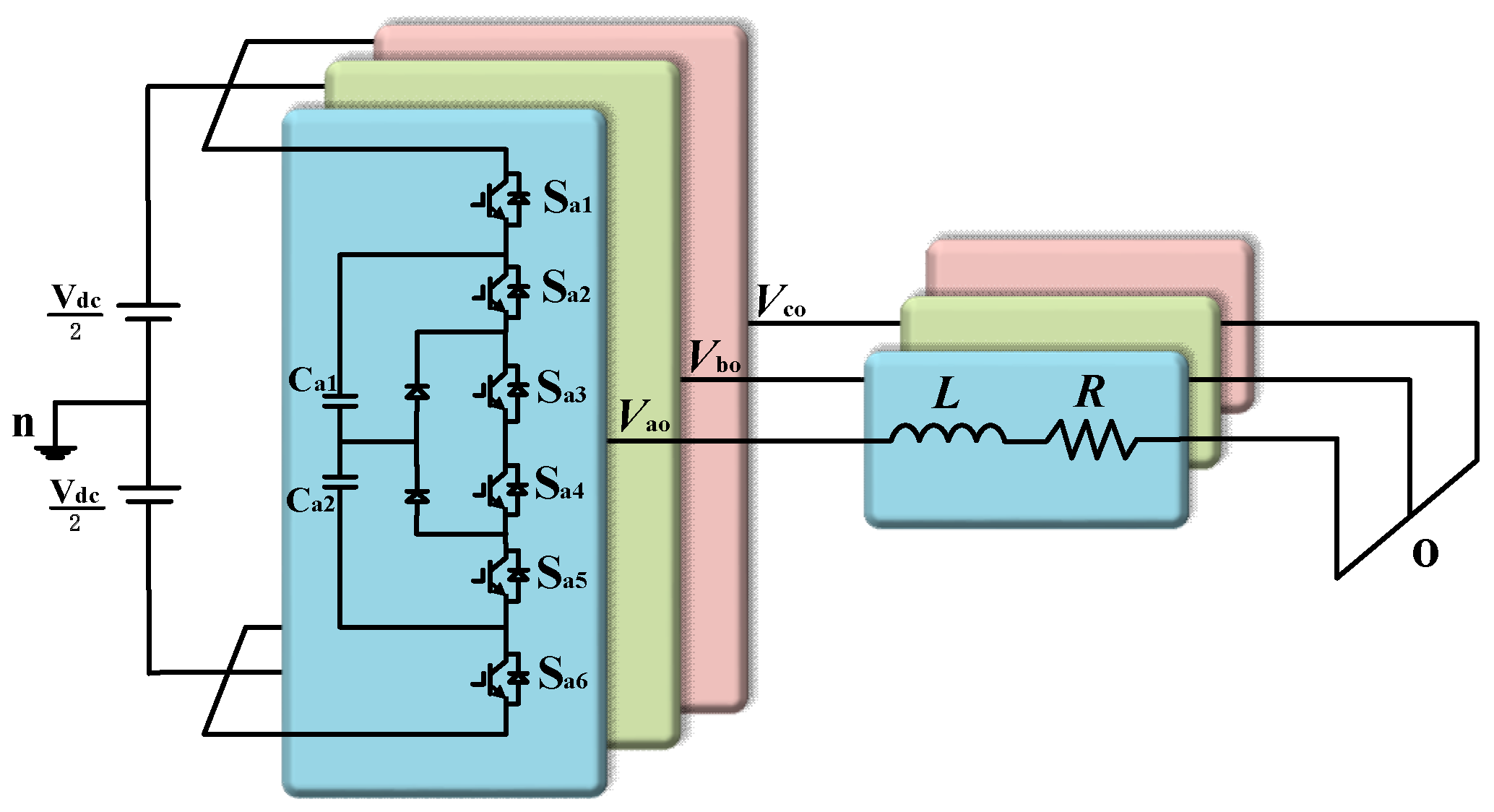
2. Operating Principle of Three Phase 4L-NNPC Inverter

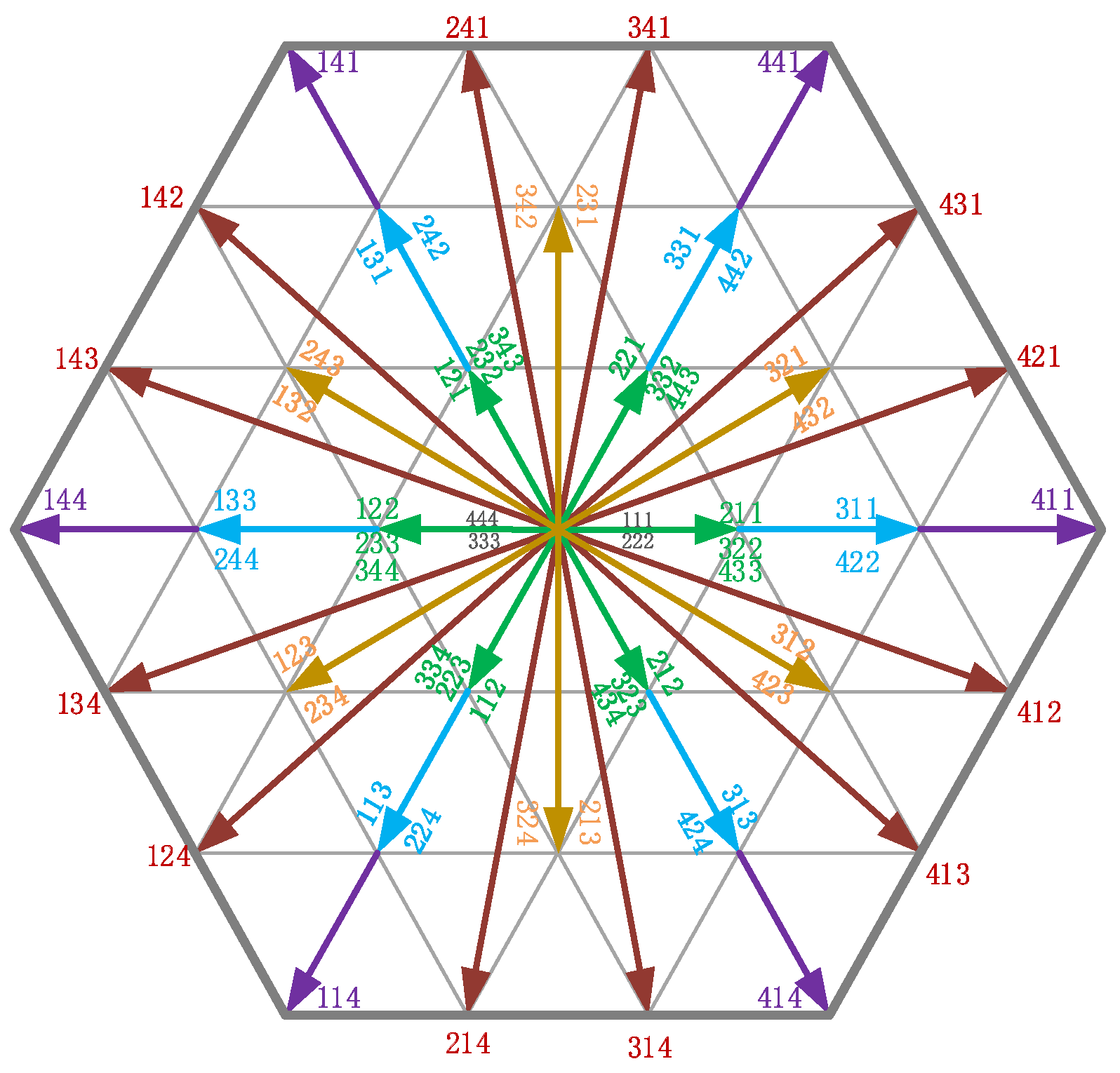
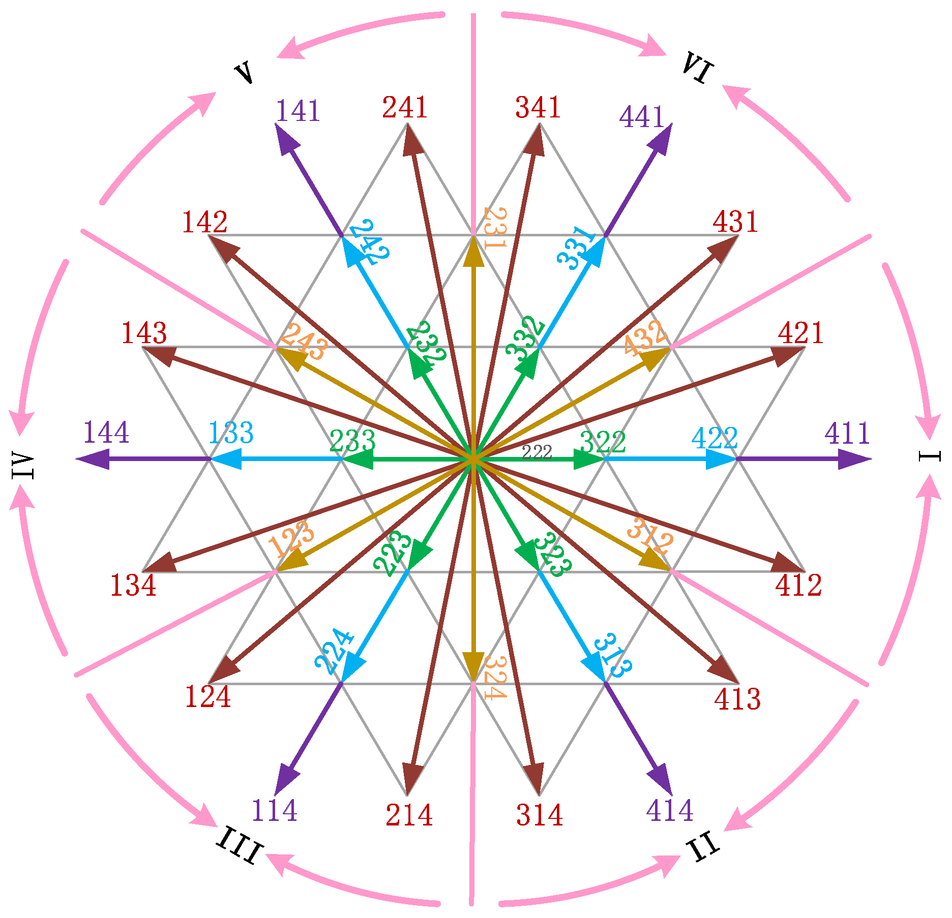
2.1. Space Vectors of 4L-NNPC

The structure of the three-phase 4L-NNPC inverter is shown in Figure 1. The arm of each phase consists of 6 IGBTs, 2 flying capacitors, and 2 diodes. When the voltage of the flying capacitor terminal stabilizes at around V_dc/3, four levels can be achieved by controlling the conduction of IGBTs, and the voltage class of the inverter can reach around 7 kV.

Taking phase A as an example, Figure 2a–f separately show the operation status of each IGBT under six switch states S(k) ∈ {4, 3a, 3b, 2a, 2b, 1}. The arrows indicate the flow path of the current, red arrows represent the current flowing into the inverter (i_x < 0), while blue represents the current flowing out (i_x > 0).

The operation of IGBTs at different levels is shown in

Table 2. Switching States of 4L-NNPC.

Phase Voltage	Level	Switching Vector	Switching State
			Sx1	Sx2	Sx3	Sx4	Sx5	Sx6
Vdc/2	4	4	1	1	1	0	0	0
Vdc/6	3	3a 3b	1 0	0 1	1 1	1 0	0 0	0 1
−Vdc/6	2	2a 2b	1 0	0 0	0 1	1 1	1 0	0 1
−Vdc/2	1	1	0	0	0	1	1	1

. According to the table, there are 6 switch states in each phase, so there is a total of 6 × 6 × 6 = 216 switch states in the three-phase system. Redundant switch states exist in voltage levels 2 and 3, which have different effects on the FCs. This property is exploited to balance the FC voltages. The proposed balance method will be described in detail in Section 3.

For the 4L-NNPC inverter, each phase can generate 4 levels of states, which are −V_dc/2, −V_dc/6, V_dc/6, and V_dc/2. Therefore, the 3-phase converter produces a total of 64 combinations of level states and transforms each combination of V_a, V_b, and V_c into a different voltage vector in the α-β frame. The 4L-NNPC voltage vector diagram is shown in Figure 3.

We use L₀, L₁, L₂, L₃, L₄, and L₅ to label vectors of different lengths, with the length increasing as the label increases. The gray numbers represent the L₀ vector, green represents L₁, orange represents L₂, blue represents L₃, red represents L₄, and purple represents L₅. The voltage vector increases from long to short, and the corresponding redundant vector increases from small to large. Among them, the L₄ and L₅ vectors have no redundant vectors, while the L₃ and L₄ vectors have one redundant vector, the L₁ and L₂ vectors have two redundant vectors, and the L₀ vector has three redundant vectors. It follows that the 4L-NNPC inverter owns a large number of space vectors, so it is necessary to adopt an appropriate vector selection method to avoid the problem of excessive computational complexity.

2.2. Dynamic Model of Output Current

From Figure 1, if the inductance value of the x-phase is defined as L_x and the resistance value is R_x, according to Kirchhoff’s voltage law (KVL), the differential equation of output current can be as follows:

$$\left\{\begin{array}{c}{L}_{\mathrm{a}}{\displaystyle \frac{d{i}_{\mathrm{a}}}{dt}}=V_{\mathrm{an}}-R_{\mathrm{a}}{i}_{\mathrm{a}}-V_{\mathrm{on}}\\ L_{\mathrm{b}}{\displaystyle \frac{d{i}_{\mathrm{b}}}{dt}}=V_{\mathrm{bn}}-R_{\mathrm{b}}{i}_{\mathrm{b}}-V_{\mathrm{on}}\\ L_{\mathrm{c}}{\displaystyle \frac{d{i}_{\mathrm{c}}}{dt}}=V_{\mathrm{cn}}-R_{\mathrm{c}}{i}_{\mathrm{c}}-V_{\mathrm{on}}\end{array}\right.$$

(1)

Then, the common-mode voltage (CMV) V_on of the 4L-NNPC inverter can be written as

$$V_{\mathrm{on}}={\displaystyle \frac{1}{3}}{\displaystyle \sum }_{\mathrm{x}=\mathrm{a},\mathrm{b},\mathrm{c}}{V}_{\mathrm{xn}}$$

(2)

By substituting (2) into (1), the matrix form of the output current can be written as

$$\left[\begin{array}{c}{\displaystyle \frac{d{i}_{\mathrm{a}}}{dt}}\\ {\displaystyle \frac{d{i}_{\mathrm{b}}}{dt}}\\ {\displaystyle \frac{d{i}_{\mathrm{c}}}{dt}}\end{array}\right]=\left[\begin{array}{c}\begin{array}{ccc}-{\displaystyle \frac{L_{\mathrm{a}}}{R_{\mathrm{a}}}}& 0& 0\end{array}\\ \begin{array}{ccc}0& -{\displaystyle \frac{L_{\mathrm{b}}}{R_{\mathrm{b}}}}& 0\end{array}\\ \begin{array}{ccc}0& 0& -{\displaystyle \frac{L_{\mathrm{c}}}{R_{\mathrm{c}}}}\end{array}\end{array}\right]\left[\begin{array}{c}{i}_{\mathrm{a}}\\ i_{\mathrm{b}}\\ i_{\mathrm{c}}\end{array}\right]+\left[\begin{array}{c}\begin{array}{ccc}{\displaystyle \frac{2}{3}}{L_{\mathrm{a}}}^{-1}& {\displaystyle \frac{1}{3}}& {\displaystyle \frac{1}{3}}\end{array}\\ \begin{array}{ccc}{\displaystyle \frac{1}{3}}& {\displaystyle \frac{2}{3}}{L_{\mathrm{b}}}^{-1}& {\displaystyle \frac{1}{3}}\end{array}\\ \begin{array}{ccc}{\displaystyle \frac{1}{3}}& {\displaystyle \frac{1}{3}}& {\displaystyle \frac{2}{3}}{L_{\mathrm{c}}}^{-1}\end{array}\end{array}\right]\left[\begin{array}{c}{V}_{\mathrm{a}}\\ V_{\mathrm{b}}\\ V_{\mathrm{c}}\end{array}\right]$$

(3)

Due to the absence of a neutral connection in the system, the output current should meet the following conditions:

$$i_{\mathrm{a}}+i_{\mathrm{b}}+i_{\mathrm{c}}=0$$

(4)

Based on the switch states shown in Table 2, the output voltage of 4L-NNPC can be characterized as follows:

$$V_{\mathrm{xn}}=\left[S_{\mathrm{x}2}-S_{\mathrm{x}1},S_{\mathrm{x}3}-S_{\mathrm{x}1},S_{\mathrm{x}1}\right]\left[\begin{array}{c}{V}_{\mathrm{cx}1}\\ V_{\mathrm{cx}2}\\ V_{\mathrm{dc}}\end{array}\right]$$

(5)

where S_x1, S_x2, and S_x3 represent the switch status of the 1/2/3 switch of phase x; when the switch is turned on, it is considered 1; and when it is turned off, it is considered 0. V_dc is the DC-link voltage. V_cx1 and V_cx2 are the voltage of the upper and lower FCs in the x phase.

Thus, the output voltage of three phases can be expressed as

$$V_{\mathrm{out}}={\displaystyle \frac{2}{3}}\left[V_{\mathrm{an}}+\gamma V_{\mathrm{bn}}+{\gamma }^2{V}_{\mathrm{cn}}\right]$$

(6)

where γ = $e^{\mathrm{j}2\pi /3}$.

According to (1), transforming a three-phase stationary reference frame to a two-phase stationary reference frame (α-β), and assuming that the three-phase load is balanced, with inductance of L and resistance of R, the continuous domain mathematical model of the three-phase system in the α-β frame can be written as

$$\left\{\begin{array}{l}{V}_{\mathsf{\alpha }}=R_{\mathsf{\alpha }}{i}_{\mathsf{\alpha }}+L_{\mathsf{\alpha }}{\displaystyle \frac{d{i}_{\mathsf{\alpha }}}{dt}}\\ V_{\mathsf{\beta }}=R_{\mathsf{\beta }}{i}_{\mathsf{\beta }}+L_{\mathsf{\beta }}{\displaystyle \frac{d{i}_{\mathsf{\beta }}}{dt}}\end{array}\right.$$

(7)

where V_α, V_β, i_α, and i_β are the output voltage and output current of the inverter, in the α-β reference frame, respectively. Using forward Euler discretization and substituting, the output current i_α and i_β are obtained as

$$\left\{\begin{array}{l}{\displaystyle \frac{d{i}_{\mathsf{\alpha }}}{dt}}={\displaystyle \frac{i_{\mathsf{\alpha }}\left(k+1\right)-i_{\mathsf{\alpha }}\left(k\right)}{T_S}} \\ {\displaystyle \frac{d{i}_{\mathsf{\beta }}}{dt}}={\displaystyle \frac{i_{\mathsf{\beta }}\left(k+1\right)-i_{\mathsf{\beta }}\left(k\right)}{T_{\mathrm{S}}}}\end{array}\right.$$

(8)

where T_S is the control period of output current. From (7) and (8), the following can be obtained:

$$\left\{\begin{array}{l}{i}_{\mathsf{\alpha }}\left(k+1\right)=i_{\mathsf{\alpha }}\left(k\right)\left(1-{\displaystyle \frac{R{T}_{\mathrm{S}}}{L}}\right)+{\displaystyle \frac{T_{\mathrm{S}}{V}_{\mathsf{\alpha }}\left(k\right)}{L}}\\ i_{\mathsf{\beta }}\left(k+1\right)=i_{\mathsf{\beta }}\left(k\right)\left(1-{\displaystyle \frac{R{T}_{\mathrm{S}}}{L}}\right)+{\displaystyle \frac{T_{\mathrm{S}}{V}_{\mathsf{\beta }}\left(k\right)}{L}}\end{array}\right.$$

(9)

By using (9), the predicted values of the output currents i_α and i_β at instant k + 1 under the action of any spatial voltage vector can be calculated at instant k.

2.3. Dynamic Model of FCs Voltages

Similar to the output current, using the forward Euler method, the upper and lower capacitor voltages V_cx1 and V_cx2 are formulated as follows:

$$\left\{\begin{array}{l}{V}_{\mathrm{cx}1}\left(k+1\right)=V_{\mathrm{cx}1}\left(k\right)+{\displaystyle \frac{{{\displaystyle T}}_{\mathrm{S}}}{{{\displaystyle C}}_1}}{i}_{\mathrm{cx}1}\left(k\right)\\ V_{\mathrm{cx}2}\left(k+1\right)=V_{\mathrm{cx}2}\left(k\right)+{\displaystyle \frac{{{\displaystyle T}}_{\mathrm{S}}}{{{\displaystyle C}}_2}}{i}_{\mathrm{cx}2}\left(k\right)\end{array}\right.$$

(10)

where V_cx1(k + 1) and V_cx2(k + 1) are the predicted values of the FC voltages at instant k + 1, i_cx1 and i_cx2 are the value of current flow into capacitor 1 and 2. But in practice, i_cx1 and i_cx2 are unable to be measured directly, so we need to relate it to i_x through a function, expressed as

$$\left\{\begin{array}{c}{i}_{\mathrm{cx}1}=\left(S_{\mathrm{x}1}-S_{\mathrm{x}2}\right)i_{\mathrm{x}}\\ i_{\mathrm{cx}2}=\left(S_{\mathrm{x}5}-S_{\mathrm{x}6}\right)i_{\mathrm{x}}\end{array}\right.$$

(11)

By substituting (11) into (10), the prediction functions of FC voltages are changed into

$$\left\{\begin{array}{l}{V}_{\mathrm{cx}1}\left(k+1\right)=V_{\mathrm{cx}1}\left(k\right)+{\displaystyle \frac{T_{\mathrm{S}}\left(S_{\mathrm{x}1}-S_{\mathrm{x}2}\right)}{C_2}}{i}_{\mathrm{x}}\left(k\right)\\ V_{\mathrm{cx}2}\left(k+1\right)=V_{\mathrm{cx}2}\left(k\right)+{\displaystyle \frac{T_{\mathrm{S}}(S_{\mathrm{x}5}-S_{\mathrm{x}6})}{C_2}}{i}_{\mathrm{x}}\left(k\right)\end{array}\right.$$

(12)

From (5), the output voltage of the 4L-NNPC inverter is related to the voltages of the six capacitors. Different switching states have different effects on the FC voltages. Their fluctuation is caused by the different components through which the current flows under different switching states. Therefore, in order to stabilize the output voltage of the 4L-NNPC inverter, it is necessary to control the FC voltages to ensure that it is stable at V_dc/3.

To facilitate understanding and further explanation of capacitor charging and discharging,

Table 3. Switching states and their impacts on FC voltage.

Phase Voltage	Switching State	FCs Voltages
		Cx1	Cx2
Vdc/2	4	No Effect	No Effect
Vdc/6	3a	Discharging (ix > 0) Charging (ix < 0)	Discharging (ix > 0) Charging (ix < 0)
	3b	Charging (ix > 0) Discharging (ix < 0)	No Effect
−Vdc/6	2a	Charging (ix > 0) Discharging (ix < 0)	Charging (ix > 0) Discharging (ix < 0)
	2b	No Effect	Discharging (ix > 0) Charging (ix < 0)
−Vdc/2	1	No Effect	No Effect

and Figure 2 show the impact of switching states on capacitors. Assuming that the current direction is positive for output, the dynamic equation of FC voltages in the x-phase is as follows:

$${\displaystyle \frac{d{V}_{\mathrm{cxm}}}{dt}}={\displaystyle \frac{1}{C}}{R}_{\mathrm{x}}{i}_{\mathrm{xm}}$$

(13)

where V_cxm and i_cxm represent the upper and lower FC voltages and current flow into capacitors. R_x is a variable representing charge and discharge. R_x = 1 stands for charge, R_x = 0 stands for no effect, R_x = −1 stands for discharge. When m = 1, it represents the upper capacitor, and when m = 2, it represents the lower one. Through the above analysis, it can be concluded that it is feasible to stabilize the voltages of each capacitor through the RSS. In the following section, the concrete balancing method of FC voltages will be discussed.

3. Proposed 3LS-MPC for 4L-NNPC Strategy

3.1. CMV Reduction Strategy

From (2), the CMV is related to the three-phase output voltage and selection of space vectors.

Table 4. Switching states and common-mode voltage of 4L-NNPC.

Common-Mode Voltage	Switch State
−Vdc/2	111
−7 Vdc/18	112 121 211
−5 Vdc/18	113 122 131 212 221 311
−Vdc/6	114 132 123 141 213 222 231 312 321 411
−Vdc/18	124 133 142 214 223 232 241 313 322 331 412 421
Vdc/18	134 143 224 233 242 314 323 332 341 413 422 431
Vdc/6	144 234 243 324 333 342 414 423 432 441
5 Vdc/18	244 334 343 424 433 442
7 Vdc/18	443 344 434
Vdc/2	444

shows the relationship between different space vectors and common-mode voltage.

There are 10 levels of ±V_dc/2, ±7 V_dc/18, ±5 V_dc/18, ±V_dc/6, and ±V_dc/18 for the 4L-NNPC inverter. According to Table 4, the relationship between the CMV and DC-link voltage can be obtained as

$$V_{\mathrm{on}}={\displaystyle \frac{2{{\displaystyle \sum }}_{\mathrm{x}=\mathrm{a},\mathrm{b},\mathrm{c}}{G}_{\mathrm{x}}-15}{18}}{V}_{\mathrm{dc}}$$

(14)

where G_x is the level state of each phase, taking values of 1, 2, 3, and 4.

The space vector diagram after removing the high-CMV vector of Figure 3 is shown in Figure 4. It is worth noting that the modulation scheme in references [31,32,33] uses high-CMV vectors, which can lead to problems such as increased motor shaft current and electromagnetic interference. If the high-CMV vectors are removed, it can be difficult to control the FC voltages when the modulation is relatively small.

To reduce the CMV, consider removing voltage vectors with CMV absolute values greater than V_dc/6. Thus, the voltage vectors that generate CMV values of ±5 V_dc/18, ±7 V_dc/18, and ±V_dc/2 all need to be removed. In addition, due to the use of the FCS-MPC strategy, all L₀ vectors can be removed. In this way, we removed 4 L₀ vectors, 12 L₁ vectors, and 6 L₃ vectors. The number of space vectors was reduced from 64 to 42. The deleted vectors can be found in Table 4.

But at this point, there is still redundancy in the L₂ vectors, and the CMV value generated by L₂ is exactly ±V_dc/6. To ensure the simplicity of the control strategy, it is necessary to remove all redundant vectors. Therefore, it is considered to remove 6 vectors: {234} {342}, and {432} (generating CMV as V_dc/6) as well as {132}, {213}, and {321} (generating CMV as −V_dc/6), so that there is no redundancy in the L₂ vectors. In summary, a total of 28 vectors were removed, and the number of spatial vectors was reduced from 64 to 36.

3.2. Switch State Disabled Strategy

It can be concluded that the control objective of stabilizing the FC voltage is mainly described as controlling the current flowing into or out of the capacitor, so that the deviation from the expected value (V_dc/3) is not too large. The deviation formula is expressed as follows:

$$\mathsf{\Delta }{V}_{\mathrm{cxm}}={\displaystyle \frac{3V_{\mathrm{cxm}}-V_{\mathrm{dc}}}{3}}$$

(15)

where ΔV_cxm is deviation value of the FC voltage; when the value is greater than 0, the RSS that can charge the capacitor should be disabled. The proposed method determines the switch state that needs to be disabled through the constructed logic function, and even if the high-CMV vectors are removed, the FC voltages is still controllable.

Since switch states 1 and 4 do not affect the charging and discharging of FCs, they will not be disabled. Considering the FC voltages deviation and phase current direction, we disabled some RSSs of levels 3 and 2.

In order to select the appropriate RSS, a strategy for setting the logic function is proposed. The logic variables PR_x(t) Dir_x(t), and Dev_cxm(t) are defined to characterize the priority of capacitors C_x1 and C_x2, direction of the phase current, and deviation of FC voltages. The logical variables are shown in (16)–(18):

$$P{R}_{\mathrm{x}}\left(t\right)=\left\{\begin{array}{c}1|\mathsf{\Delta }{V}_{\mathrm{cx}1}\left(t\right)|\ge |\mathsf{\Delta }{V}_{\mathrm{cx}2}\left(t\right)|\\ 0|\mathsf{\Delta }{V}_{\mathrm{cx}1}\left(t\right)|<|\mathsf{\Delta }{V}_{\mathrm{cx}2}\left(t\right)|\end{array}\right.$$

(16)

$$Di{r}_{\mathrm{x}}\left(t\right)=\left\{\begin{array}{c}1i_{\mathrm{x}}\left(t\right)\ge 0\\ 0i_{\mathrm{x}}\left(t\right)<0\end{array}\right.$$

(17)

$$\begin{array}{l}De{v}_{\mathrm{cx}1}\left(t\right)=\left\{\begin{array}{c}1 \mathsf{\Delta }{V}_{\mathrm{cx}1}>0\\ 0 \mathsf{\Delta }{V}_{\mathrm{cx}1}<0\end{array} \right.\\ De{v}_{\mathrm{cx}2}\left(t\right)=\left\{\begin{array}{c}1 \mathsf{\Delta }{V}_{\mathrm{cx}1}>0\\ 0 \mathsf{\Delta }{V}_{\mathrm{cx}2}<0\end{array} \right.\end{array}$$

(18)

Using the logical variables described above, the logical function for disabling the RSS BC_x can be derived as

$$B{C}_{\mathrm{x}}=P{R}_{\mathrm{x}}(Dir\mathrm{x}\odot Dev\mathrm{cx}1)|\overline{P{R}_{\mathrm{x}}}(Dir\mathrm{x}\odot Dev\mathrm{cx}1), B{C}_{\mathrm{x}}=\left\{\begin{array}{l}1\mathrm{disable}\mathrm{RSS}3a2\mathrm{b}\\ 0\mathrm{disable}\mathrm{RSS}3b2\mathrm{a}\end{array}\right.$$

(19)

The proposed switching state disabling method features a more streamlined algorithmic implementation compared to conventional approaches. The following will provide an example to illustrate the process of disabling an RSS. Assuming that the deviation ΔV_cx1 > 0 at instant t₁, if Pr (t₁) is 1, the main purpose is to stabilize the voltage of C_x1. If the current direction is positive at this time, it is necessary to disable the switch state that charges C_x1 or keeps it unchanged. Therefore, switch states 3b and 2a are disabled. Therefore, the RSS can be disabled through (19) to balance the FC voltages.

3.3. Optimal Vector Selection

To achieve high-quality output current and FC voltage balance control for the three-phase 4L-NNPC inverter, the cost function of the classical FCS-MPC algorithm usually includes two control objectives, including output current and FC balance, expressed as

$$g_1=\left|i_{\mathsf{\alpha }}^{*}\left(k+1\right)-i_{\mathsf{\alpha }}\left(k+1\right)\right|+\left|i_{\mathsf{\beta }}^{*}\left(k+1\right)-i_{\mathsf{\beta }}\left(k+1\right)\right|+\lambda {\displaystyle \sum }_{\mathrm{x}=\mathrm{a},\mathrm{b},\mathrm{c}}{{\displaystyle \sum }}_{j=1}^2\left|V_{\mathrm{cref}}-V_{\mathrm{cxj}}\left(k+1\right)\right|$$

(20)

where λ is the weighting factor for stabilizing the voltage of each capacitor, and V_cjref is the reference voltage of each capacitor, which is V_dc/3 in this paper. i^*_α(k + 1) and i^*_β(k + 1) are reference current of k + 1 instant, and they can be obtained from the Lagrange extrapolation and Clarke transformation at time k, k − 1, and k − 2, with the extrapolation formula as

$$i_{\mathrm{x}}^{*}\left(k+1\right)=3i_{\mathrm{x}}^{*}\left(k\right)-3i_{\mathrm{x}}^{*}\left(k-1\right)+i_{\mathrm{x}}^{*}\left(k-2\right)\left(\mathrm{x}=\mathrm{a},\mathrm{b},\mathrm{c}\right)$$

(21)

The classic FCS-MPC method requires substituting 64 vectors into (20) to select the optimal vector. The classical strategy requires many iterations during operation, especially in the case of multi-level inverters. The number of vectors is the fourth power of the number of levels, which greatly increases the computational burden and reduces the quality of the output current. In addition, the weight factor λ used to stabilize the FC voltages is usually tuned using trial-and-error methods, which is difficult to implement, and currently there is no systematic and universally applicable method for determining it. Given that the 4L-NNPC inverter possesses RSSs that can be utilized to balance the voltage of FCs, it is not necessary to employ weighting factors to stabilize the FC voltages.

The cost function g of the proposed 3LS-MPC control strategy is given as follows:

$$g=\left|i_{\mathsf{\alpha }}^{*}\left(k+1\right)-i_{\mathsf{\alpha }}\left(k+1\right)\right|+\left|i_{\mathsf{\beta }}^{*}\left(k+1\right)-i_{\mathsf{\beta }}\left(k+1\right)\right|$$

(22)

In (22), the cost function is used for the second and third stages of MPC. In each control cycle of system operation, after disabling RSSs, (22) is used to select one of the L₃ vectors ({422}, {331}, {242}, {133}, {224}, and {313}) to determine the sector where the reference voltage vector is located. The advantage of this approach over other sequential control methods lies in the reduced number of vectors required to be selected within each small sector (from 9 to 7). Finally, an optimal vector is selected from the 7 voltage vectors in the small sector according (22) again.

The control diagram of the proposed 3LS-MPC strategy is shown in Figure 5. Compared to classical algorithms, the proposed 3LS-MPC algorithm eliminates weighting factor and reduces common-mode voltage, consisting of five steps:

(1)

Sample the three-phase output current i_abc(k) at instant k and the DC-side midpoint voltage U_o(k).

(2)

Perform the Clarke transformation of the output current i_abc(k) from the three-phase stationary coordinate system to the two-phase stationary coordinate system to obtain the currents i_α(k) and i_β(k) in the α-β frame.

(3)

Using the method of logical function, the disabled RSSs are selected through (19).

(4)

Estimate i^*_α(k + 1), i^*_β(k + 1) by Lagrange extrapolation (21), and estimate i_α(k + 1), i_β(k + 1), V_cx1(k + 1), and V_cx2(k + 1) by prediction Equations (9) and (12).

(5)

Substitute i^*_α(k + 1), i^*_β(k + 1), i_α(k + 1), and i_β(k + 1) into the control set containing 6 L₃ voltage vectors, and perform cyclic iteration using the cost function (22) to find the voltage vector that minimizes the cost function value, obtaining the sector where the reference vector is located accordingly.

(6)

After determining the sector, select the basic voltage vector with the minimum cost function value among the 6 candidate vectors using (22) in the same way as step (5) to obtain the optimal vector.

4. Simulation Results and Analysis

To verify the feasibility of the proposed method, a 3PH system of 3.3 MVA was constructed in Matlab/Simulink 2019b, with a DC-side voltage of 9.9 kV. The simulation parameter settings of the system are shown in

Table 5. Parameters of simulation and experiment.

Parameter	Symbol	Simulation	Experimental
Total DC voltage (V)	Vdc	9900	240
Flying capacitance (μF)	Cx1/Cx2	4700	1150
Load inductance (mH)	L	10	8
Load resistance (Ω)	R	6	3
Sample period (ms)	Ts	0.1	0.1
Nominal voltage (V)	Vn	6100	150
Nominal power (kW)	Pn	3330	2.8
Nominal frequency (Hz)	fn	50	50
Switching frequency (kHz)	fs	10	10

, and the performance of the controller is examined in both steady-state and transient conditions.

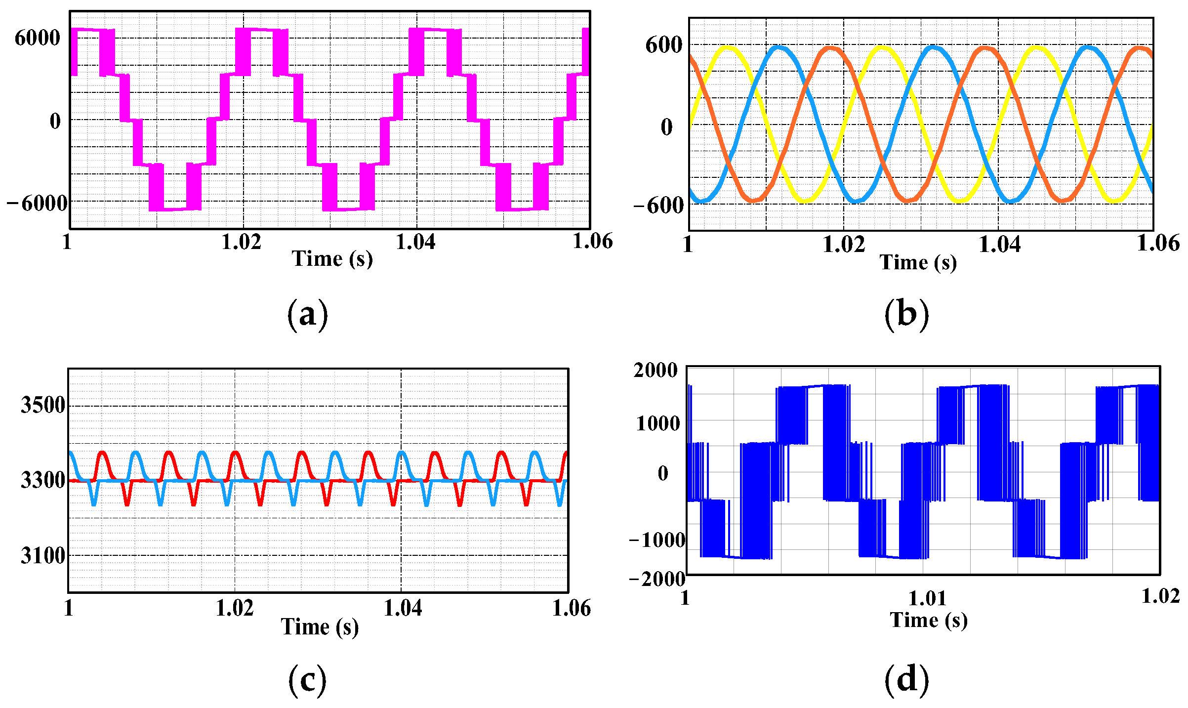
4.1. Steady-State Analysis of Simulation

In the steady-state simulation, the rated current is 580 A. First, a steady-state simulation was conducted on the proposed method, with a balanced three-phase load, as shown in Figure 6a,b. It can be observed from these figures that the current is almost the same as the reference value, and the voltage exhibits a steady change in a stepped waveform. In Figure 6c, the fluctuations in the FC voltage are relatively regular and stable. Typically, the maximum permissible ripple should not exceed 10%, and the simulation results indicate a ripple of approximately 4.3%, with no evident abnormal fluctuations, indicating good steady-state performance.

Secondly, the simulation analyzed the CMV and THD of the system. As shown in Figure 6d, in classic methods, the CMV can potentially reach 3580 V, equivalent to 7 V_dc/18, and the CMV of the proposed method is consistently below 1650 V, equivalent to V_dc/6. It can be concluded that the proposed method reduces CMV by 57.14%. According to Figure 7, the THD of the A-phase output current is only 1.15%, further indicating the superior output performance.

4.2. Dynamic-State Analysis of Simulation

The simulation also conducted some analyses on the dynamic performance of the system. A step signal was applied to the reference current from 580 A to 460 A within 2 s, a decrease of approximately 20% of the reference current value. Figure 8a indicates that the system’s dynamic response is relatively rapid. The output currents become stable within a quarter of a cycle. From Figure 8b, it can be observed that although the fluctuation amplitude of the FC voltage increases with the reduction in the load, the maximum ripple remains within approximately 6%, and no significant deviation occurs.

Based on the results obtained from the simulation, it can be demonstrated that the proposed method not only satisfies FC voltage balance but also reduces CMV. Furthermore, by using the sequential MPC strategy, the number of vector traversals is reduced. Compared to the classical FCS-MPC, it reduces the computational burden.

5. Experimental Results

Based on the simulation results, an inverter main circuit and control system, as shown in Figure 9, were built on a hardware experimental platform, using a digital controller with a TMS320F28379D digital signal processor (DSP). The IGBT of IHW30N65R5 is adopted as the power switch of the inverter, and the driver IC is 1EDI20I12AF. The type of voltage/current sensors is CHV-25P/CHG-10AE. The sampling frequency is 10 kHz. The other experimental parameters are presented in Table 4, with the inverter output connected to a three-phase star-shaped resistive load. Experimental analysis and comparison were conducted between the classical FCS-MPC algorithm (with weighting factor) and proposed 3LS-MPC algorithm in this paper. The experiment primarily assesses various performance metrics, including output current, harmonic content, the stability of FC voltage, and CMV.

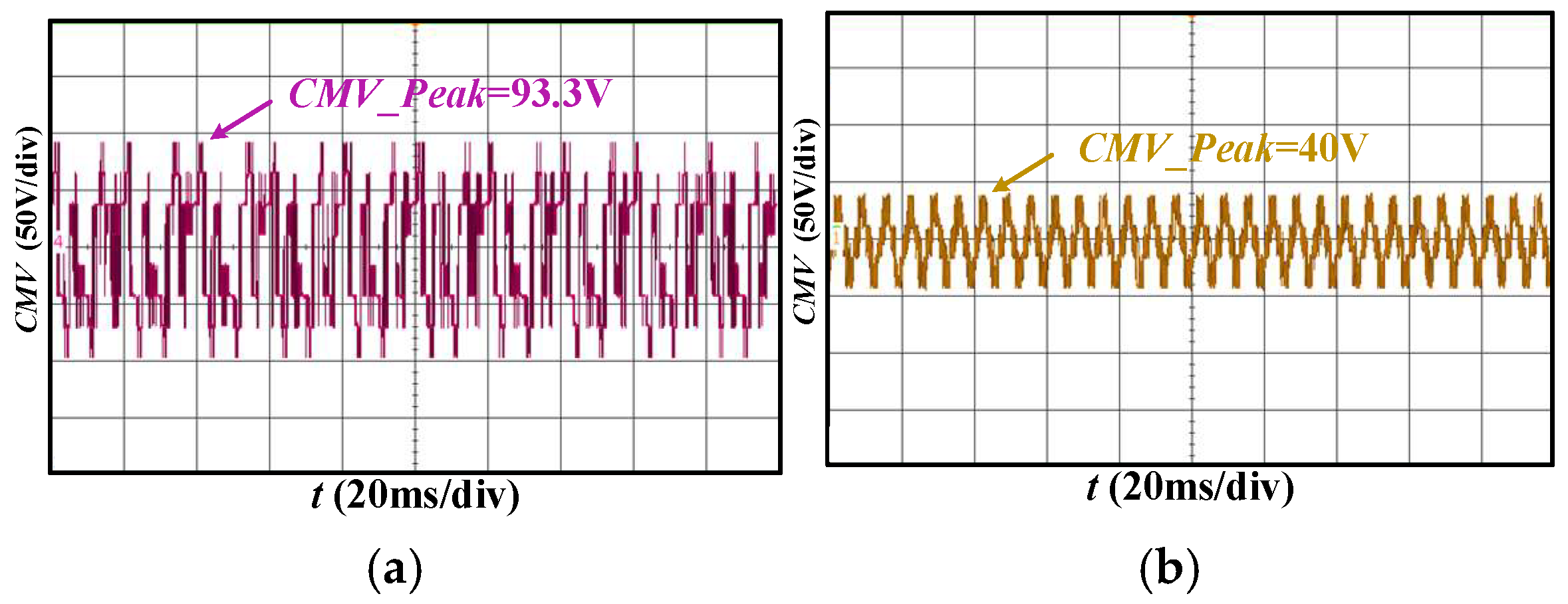
5.1. Comparative Steady-State Analysis of Proposed 3LS-MPC and FCS-MPC Methods

Aiming to verify the effectiveness of the two MPCC algorithms, systematic steady-state experiments were conducted on each method. For ease of expression, the classical FCS-MPC method with a weighting factor is referred to as the “classical method”. Taking into account both steady-state and dynamic performances, the weighting factor in the classical method is set to 0.15 by experience design.

This experiment examined the steady-state operation of the 4L-NNPC inverter at base frequency (50 Hz) with an output current amplitude of 1.5 A and 2.4 A. Figure 10, Figure 11 and Figure 12 illustrate the experimental results for three-phase output currents, line–line output voltage U_ab, FC voltages, and the CMV. In addition,

Table 6. Performances of two MPC methods.

Methods	Amplitude of iref	THD	ΔVpa
Classical Method	1.5 A	2.90%	6 V
	2.4 A	3.22%	6 V
Proposed Method	1.5 A	2.74%	4 V
	2.4 A	2.97%	4 V

is used to compare the steady-state performance of the two methods. ΔV_pa is the peak-to-peak ripple of phase-A FC voltages.

In Figure 10, the output currents of both methods are sinusoidal with high quality. According to Table 6, the proposed method exhibits a smaller THD at a switching frequency of 10 kHz. Therefore, the proposed method offers slightly better current waveform quality compared to the classical approach.

From Figure 11, it can be observed that while both methods can maintain the stability of the FC voltage under the specified condition, the proposed method, whether it is U_ca1 or U_ca2, maintains a maximum voltage ripple of less than 5%, while the voltage ripple of the classical method is greater than 7%. It shows that even without weighting factors, solely relying on logical functions for capacitor voltage balance, at a standard output frequency of 50 Hz, the proposed method exhibits excellent performance comparable to that of the classical approach. Therefore, it can be concluded that under the standard 50 Hz working condition, removing the weighting factor will not lead to the instability of FCs.

Furthermore, the experiment examined the waveform of the CMV under both methods, as illustrated in Figure 12. The peak value of the CMV for the classical approach reached 93.3 V, approximately 7/18 V_dc. In contrast, the proposed method, due to the removal of voltage vectors that can generate high CMVs, resulted in a peak CMV of only 60 V, approximately V_dc/6. This reduction in the peak value is expected to mitigate electromagnetic interference (EMI) that may be generated by the device in practical applications.

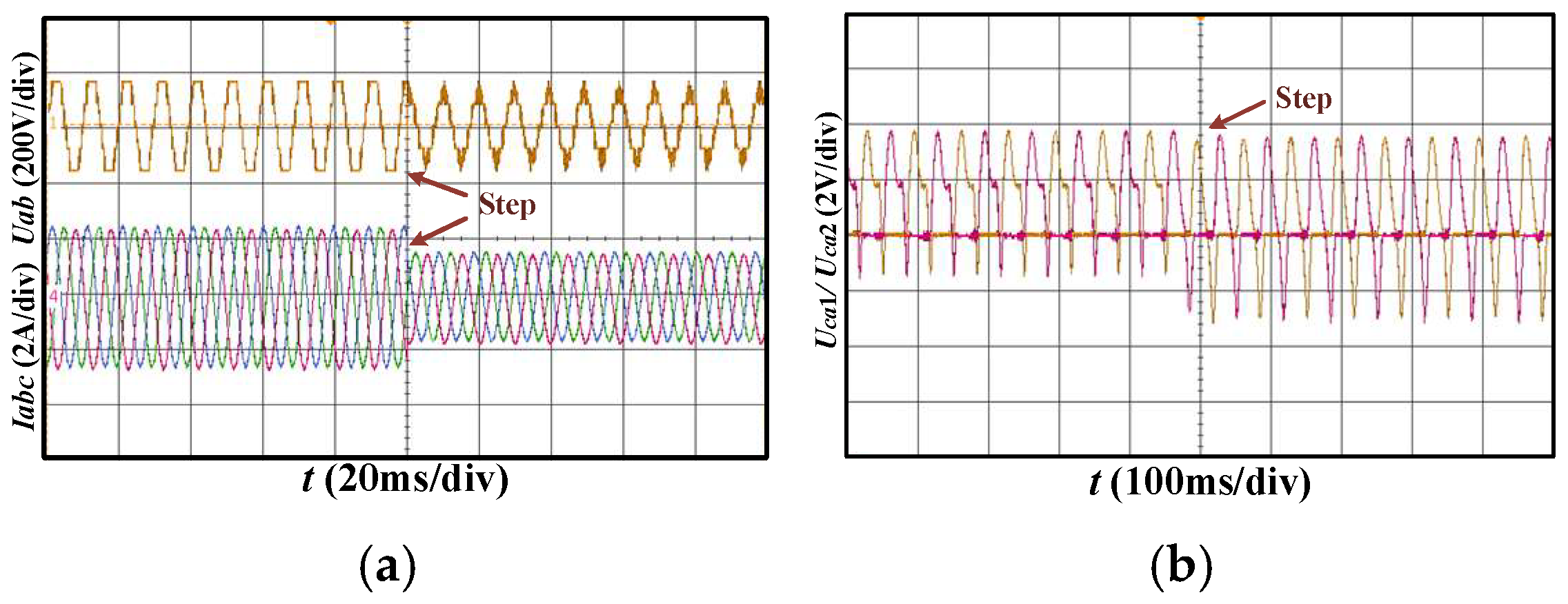
5.2. Dynamic-State Analysis of Experiment

In dynamic experiments, similar to simulations, the reference current changed in a step-wise manner from 2.4 A to 1.5 A, as shown in Figure 13a,b. Line voltage, three-phase current, and FC voltage are displayed. After a relatively minor fluctuation, the voltage and current stabilized, and the FC voltage remained stable at approximately 80 V, with a larger fluctuation than before the change, but the ripple remained below 10%. Overall, the results are relatively similar to those obtained from simulations.

In summary, the comparison of steady-state experimental results shows that the proposed 3LS-MPC method reduces the computational burden and has excellent performance, while stabilizing the FC voltage, which is beneficial for the output voltage stability of distributed renewable energy generation systems. The dynamic experimental results show that the system can still meet all performance indicators when the load changes, and the switching process is relatively fast.

6. Conclusions

This paper proposes a three-layer sequential MPC method, simultaneously achieving the balance of FC voltages and a reduction in the CMV. In this approach, 28 vectors that generated high CMV were removed. Before space vector selection, the switching state that further offsets the FC voltages are disabled, followed by identifying the optimal sector. Finally, the optimal vector is chosen within the selected sector to minimize the FC voltage fluctuation and output current errors. Through this method, the self-balance of FCs is achieved, enhancing system performance and reducing the CMV. The experimental results show that the three-phase system has good dynamic and static performance. In future research work, its application in grid-connected systems can be further considered.

References

1. Chen, Y.; Li, H.; Jin, T. A Novel High-Boost Interleaved DC-DC Converter for Renewable Energy Systems. Prot. Control Mod. Power Syst. 2025, 10, 132–147. [Google Scholar] [CrossRef]
2. Li, H.; Chen, Y.; Jin, T. A soft-switched SEPIC-based high voltage gain DC-DC converter for renewable energy applications. IEEE Trans. Ind. Electron. 2025, 72, 3746–3757. [Google Scholar] [CrossRef]
3. Zhang, Z.; Xu, Y.; Yuan, Y.; Cao, H.; Liu, P.; Jin, T. Reconfiguration on Novel Unbalance Levels Strategy Adopted in a Three-Level Bidirectional LLC Resonant Converter in HESS to EV Endurance Scheme. IEEE Trans. Transp. Electrif. 2025, 11, 4906–4919. [Google Scholar] [CrossRef]
4. Lin, M.; Feng, C.; Chen, Y.; Li, H.; Jin, T. Hybrid Current Stress Optimization Strategy for Three-Level Dual Active Bridge Adapted to Wide Voltage Ranges. IEEE Trans. Power Electron, 2025; 1–13. [Google Scholar] [CrossRef]
5. Peng, Y.; Li, Y.; Lee, K.Y.; Tan, Y.; Cao, Y.; Wen, M. Coordinated Control Strategy of PMSG and Cascaded H-Bridge STATCOM in Dispersed Wind Farm for Suppressing Unbalanced Grid Voltage. IEEE Trans. Sustain. Energy 2021, 12, 349–359. [Google Scholar] [CrossRef]
6. Tang, Y.; Zhang, Z.; Xu, Z. DRU Based Low Frequency AC Transmission Scheme for Offshore Wind Farm Integration. IEEE Trans. Sustain. Energy 2021, 12, 1512–1524. [Google Scholar] [CrossRef]
7. Manoj, P.; Annamalai, K.; Dhara, S.; Somasekhar, V.T. A Quasi-Z-Source-Based Space-Vector-Modulated Cascaded Four-Level Inverter for Photovoltaic Applications. IEEE J. Emerg. Sel. Top. Power Electron. 2022, 10, 4749–4762. [Google Scholar]
8. Vinod, B.R.; Shiny, G. Direct Torque Control Scheme for a Four-Level-Inverter Fed Open-End-Winding Induction Motor. IEEE Trans. Energy Convers. 2019, 34, 2209–2217. [Google Scholar]
9. Liu, X.; Qiu, L.; Wu, W.; Ma, J.; Wang, D.; Peng, Z.; Fang, Y. Finite-time ESO-based cascade-free FCS-MPC for NNPC converter. Int. J. Electron. Power Energy Syst. 2023, 148, 108939. [Google Scholar] [CrossRef]
10. Wu, W.; Wang, D. An Optimal Voltage-Level Based Model Predictive Control Approach for Four-Level T-Type Nested Neutral Point Clamped Converter With Reduced Calculation Burden. IEEE Access 2019, 7, 87458–87468. [Google Scholar] [CrossRef]
11. Narimani, M.; Wu, B.; Cheng, Z.; Zargari, N.R. A New nested Neutral Point Clamped (NNPC) Converter for Medium-Voltage (MV) Power Conversion. IEEE Trans. Power Electron. 2014, 29, 6375–6382. [Google Scholar] [CrossRef]
12. Tian, K.; Wu, B.; Narimani, M.; Xu, D.; Cheng, Z.; Zargari, N.R. A Capacitor Voltage-Balancing Method for Nested Neutral Point Clamped (NNPC) Inverter. IEEE Trans. Power Electron. 2016, 31, 2575–2583. [Google Scholar] [CrossRef]
13. Bahrami, A.; Narimani, M. A Sinusoidal Pulsewidth Modulation (SPWM) Technique for Capacitor Voltage Balancing of a Nested T-Type Four-Level Inverter. IEEE Trans. Power Electron. 2019, 34, 1008–1012. [Google Scholar] [CrossRef]
14. Wu, M.; Li, Y.W.; Tian, H.; Li, Y.; Wang, K. Modified Carrier-Overlapped PWM with Balanced Capacitors and Eliminated Dead-Time Spikes for Four-Level NNPC Converters Under Low Frequency. IEEE J. Emerg. Sel. Top. Power Electron. 2022, 10, 6832–6844. [Google Scholar] [CrossRef]
15. Tan, L.; Wu, B.; Sood, V.; Xu, D.; Narimani, M.; Cheng, Z.; Zargari, N.R. A Simplified Space Vector Modulation for Four-Level Nested Neutral-Point Clamped Inverters with Complete Control of Flying-Capacitor Voltages. IEEE Trans. Power Electron. 2018, 33, 1997–2006. [Google Scholar] [CrossRef]
16. Xu, Y.; Zou, Z.; Liu, Y.; Zeng, Z.; Zhou, S.; Jin, T. Deep Learning-Based Multi-feature Fusion Model for Accurate Open-Circuit Fault Diagnosis in Electric Vehicle DC Charging Piles. IEEE Trans. Transp. Electrif. 2025, 11, 2243–2254. [Google Scholar] [CrossRef]
17. Li, X.; Xie, M.; Ji, M.; Yang, J.; Wu, X.; Shen, G. Restraint of Common-Mode Voltage for PMSM-Inverter Systems with Current Ripple Constraint Based on Voltage-Vector MPC. IEEE J. Emerg. Sel. Top. Ind. Electron. 2023, 4, 688–697. [Google Scholar] [CrossRef]
18. Monfared, K.K.; Iman-Eini, H.; Neyshabouri, Y.; Liserre, M. Model Predictive Control with Reduced Common-Mode Voltage Based on Optimal Switching Sequences for Nested Neutral Point Clamped Inverter. IEEE Trans. Ind. Electron. 2024, 71, 27–38. [Google Scholar] [CrossRef]
19. Le, Q.A.; Lee, D.-C. Reduction of Common-Mode Voltages for Five-Level Active NPC Inverters by the Space-Vector Modulation Technique. IEEE Trans. Ind. Appl. 2017, 53, 1289–1299. [Google Scholar] [CrossRef]
20. Guo, F.; Diab, A.M.; Yeoh, S.S.; Yang, T.; Bozhko, S.; Wheeler, P. An Advanced Dual-Carrier-Based Multi-Optimized PWM Strategy of Three-Level Neutral-Point-Clamped Converters for More-Electric-Aircraft Applications. IEEE Trans. Energy Convers. 2024, 39, 356–367. [Google Scholar] [CrossRef]
21. Kouro, S.; Malinowski, M.; Gopakumar, K.; Pou, J.; Franquelo, L.; Wu, B.; Rodriguez, J.; Perez, M.; Leon, J. Recent advances and industrial applications of multilevel converters. IEEE Trans. Ind. Electron. 2010, 57, 2553–2580. [Google Scholar] [CrossRef]
22. Sudha, V.; Vijayarekha, K.; Sidharthan, R.K.; Prabaharan, N. Combined Optimizer for Automatic Design of Machine Learning-Based Fault Classifier for Multilevel Inverters. IEEE Access 2022, 10, 121096–121108. [Google Scholar] [CrossRef]
23. Orfi Yeganeh, M.S.; Sarvi, M.; Blaabjerg, F.; Davari, P. Improved harmonic injection pulse-width modulation variable frequency triangular carrier scheme for multilevel inverters. IET Power Electron. 2020, 13, 3146–3154. [Google Scholar] [CrossRef]
24. Yang, Y.; Yu, H.; Li, C.; Lang, X.; Yeoh, S.S. Improved Model Predictive Current Control for Three-Phase Three-Level Converters with Neutral-Point Voltage Ripple and Common Mode Voltage Reduction. IEEE Trans. Energy Convers. 2021, 36, 3053–3062. [Google Scholar] [CrossRef]
25. Wang, Q.; Yu, H.; Li, C.; Lang, X.; Yeoh, S.S.; Yang, T.; Rivera, M.; Bozhko, S.; Wheeler, P. A Low-Complexity Optimal Switching Time-Modulated Model-Predictive Control for PMSM With Three-Level NPC Converter. IEEE Trans. Transport. Electrific. 2020, 6, 1188–1198. [Google Scholar] [CrossRef]
26. Narimani, M.; Wu, B.; Yaramasu, V.; Cheng, Z.; Zargari, N.R. Finite Control-Set Model Predictive Control (FCS-MPC) of Nested Neutral Point-Clamped (NNPC) Converter. IEEE Trans. Power Electron. 2015, 30, 7262–7269. [Google Scholar] [CrossRef]
27. Yaramasu, V.; Wu, B. Model Predictive Decoupled Active and Reactive Power Control for High-Power Grid-Connected Four-Level Diode-Clamped Inverters. IEEE Trans. Ind. Electron. 2014, 61, 3407–3416. [Google Scholar] [CrossRef]
28. Monfared, K.K.; Neyshabouri, Y.; Iman-Eini, H.; Liserre, M. An Improved Finite Control-Set Model Predictive Control for Nested Neutral Point Clamped Converter. IEEE Trans. Ind. Electron. 2023, 70, 5386–5398. [Google Scholar] [CrossRef]
29. Prajapati, D.; Dekka, A.; Ronanki, D.; Rodriguez, J. High-Performance Sequential Model Predictive Control of a Four-Level Inverter for Electric Transportation Applications. IEEE J. Emerg. Sel. Top. Ind. Electron. 2024, 5, 253–262. [Google Scholar] [CrossRef]
30. Ni, Z.; Narimani, M.; Rodriguez, J. Model Predictive Control of a Four-Level T-NNPC Inverter without Weighting Factors. In Proceedings of the IEEE Applied Power Electronics Conference and Exposition (APEC), Phoenix, AZ, USA, 14–17 June 2021; pp. 2133–2138. [Google Scholar]
31. Tan, L.; Wu, B.; Narimani, M.; Xu, D.; Liu, J.; Cheng, Z. A space virtual-vector modulation with voltage balance control for nested neutral-point clamped converter under low output frequency conditions. IEEE Trans. Power Electron. 2017, 32, 3458–3466. [Google Scholar] [CrossRef]
32. Tan, L.; Wu, B.; Narimani, M.; Xu, D.; Joos, G. Multicarrier-based PWM strategies with complete voltage balance control for NNPC inverters. IEEE Trans. Ind. Electron. 2018, 65, 2863–2872. [Google Scholar] [CrossRef]
33. Tian, H.; Li, Y.W. Carrier-based stair edge PWM (SEPWM) for capacitor balancing in multilevel converters with floating capacitors. IEEE Trans. Ind. Appl. 2018, 54, 3440–3452. [Google Scholar] [CrossRef]
Figure 1. Structure of three-phase 4L-NNPC.
Electronics 14 02910 g001
Figure 2. Switching states of (a) 4, (b) 3a, (c) 3b, (d) 2a, (e) 2b, and (f) 1 in 4L-NNPC.
Electronics 14 02910 g002
Figure 3. Space vector diagram of 4L-NNPC inverter.
Electronics 14 02910 g003
Figure 4. Thirty-seven voltage vectors with reducing CMV.
Electronics 14 02910 g004
Figure 5. Control block diagram of proposed MPCC.
Electronics 14 02910 g005
Figure 6. Steady-state simulation of the 4L-NNPC inverter: (a) output line voltage Uab, (b) output three-phase current, ia(yellow), ib(blue), and ic(red). (c) waveforms of Uca1 (red) and Uca2 (blue), and (d) CMV of the proposed method.
Electronics 14 02910 g006
Figure 7. Frequency spectrum of the A-phase current.
Electronics 14 02910 g007
Figure 8. Step changes in reference currents from 580 A to 460 A. (a) Output three-phase current, ia(yellow), ib(blue), and ic(red). (b) Waveforms of Uca1 (red) and Uca2 (blue).
Electronics 14 02910 g008
Figure 9. Experimental setup.
Electronics 14 02910 g009
Figure 10. Experimental results of line voltage Uab and three-phase current Iabc: (a) classical method 3LS-MPC in 1.5 A, (b) 3LS-MPC in 1.5 A, (c) classical method in 2.4 A, and (d) 3LS-MPC in 2.4 A.
Electronics 14 02910 g010
Figure 11. FC voltages of phase A: (a) classical method and (b) proposed 3LS-MPC.
Electronics 14 02910 g011
Figure 12. Experimental results of CMV: (a) classical method and (b) 3LS-MPC method.
Electronics 14 02910 g012
Figure 13. Step changes in reference currents from 2.4 A to 1.5 A for 3LS-MPC: (a) Uab and Iabc and (b) FC voltage of phase A.
Electronics 14 02910 g013