A Wi-Fi Fingerprinting Indoor Localization Framework Using Feature-Level Augmentation via Variational Graph Auto-Encoder

Abstract

Wi-Fi fingerprinting is a widely adopted technique for indoor localization in location-based services (LBS) due to its cost-effectiveness and ease of deployment using existing infrastructure. However, the performance of these systems often suffers due to missing received signal strength indicator (RSSI) measurements, which can arise from complex indoor structures, device limitations, or user mobility, leading to incomplete and unreliable fingerprint data. To address this critical issue, we propose Feature-level Augmentation for Localization (FALoc), a novel framework that enhances Wi-Fi fingerprinting-based localization through targeted feature-level data augmentation. FALoc uniquely models the observation probabilities of RSSI signals by constructing a bipartite graph between reference points and access points, which is then processed by a variational graph auto-encoder (VGAE). Based on these learned probabilities, FALoc intelligently imputes likely missing RSSI values or removes unreliable ones, effectively enriching the training data. We evaluated FALoc using an MLP (Multi-Layer Perceptron)-based localization model on the UJIIndoorLoc and UTSIndoorLoc datasets. The experimental results demonstrate that FALoc significantly improves localization accuracy, achieving mean localization errors of 7.137 m on UJIIndoorLoc and 7.138 m on UTSIndoorLoc, which represent improvements of approximately 12.9% and 8.6% over the respective MLP baselines (8.191 m and 7.808 m), highlighting the efficacy of our approach in handling missing data.

1. Introduction

The proliferation of location-based services (LBSs) and the rise of smart environments have fueled a significant demand for accurate and reliable indoor localization systems. Among various indoor positioning technologies, Wi-Fi-based localization has become a widely adopted solution due to its low deployment cost and ease of implementation by leveraging existing Wi-Fi infrastructure in wireless local area networks (WLANs). In particular, Wi-Fi fingerprinting, which utilizes standard signal measurements such as the received signal strength indicator (RSSI) from each Access Point (AP), has gained considerable popularity for its practicality, cost-effectiveness, and relatively straightforward implementation [1].

Wi-Fi fingerprinting typically consists of two phases: an offline phase and an online phase. In the offline phase, RSSI measurements are collected from wireless access points (WAPs) at predefined reference locations, known as reference points (RPs). The collected RSSI values, in combination with the location information of the RPs, are utilized to construct a radio map that characterizes the signal environment of the target area. In the online phase, when a user attempts to estimate their location, their device measures current RSSI values from the surrounding WAPs. These measurements are then compared with the pre-constructed radio map to determine the user’s location.

Machine learning (ML) techniques have been extensively employed in the online phase for location determination. Support vector machine (SVM)-based localization methods [2,3,4,5] learn signal patterns from RSSI data and classify them using hyperplanes; however, they can suffer from slow training and inference times, particularly with large-scale or high-dimensional datasets. Random forest (RF) has been utilized in studies [6,7,8,9] due to its proficiency in handling large-scale fingerprint datasets by leveraging multiple decision trees, though it still requires significant computational resources during training. Weighted k-nearest neighbor (WKNN)-based methods [10,11,12] offer advantages in terms of computational efficiency and implementation simplicity. However, they are sensitive to environmental changes and are often limited in their ability to capture the complex, non-linear relationship between RSSI values and physical locations [13]. Recent advancements in computational capabilities, coupled with improvements in data availability, have paved the way for deep learning (DL)applications in Wi-Fi fingerprinting. Techniques employing autoencoders, convolutional neural networks (CNN), and recurrent neural networks (RNN) have been effectively applied to learn intricate and sequential patterns in RSSI data, thereby significantly enhancing localization accuracy and flexibility [14,15,16,17,18].

Effective application of ML and DL techniques requires both sufficient quantity and high quality of training data. However, in real-world deployment scenarios, maintaining a sufficient volume of up-to-date fingerprint data is challenging, as the periodic recollection process is labor-intensive and time-consuming. This makes it difficult to sustain high-quality signal maps in dynamic environments, especially under real-time or batch processing constraints. To address this, prior research has primarily focused on two strategies. The first involves employing learning algorithms adept at handling data scarcity, such as semi-supervised [19] and unsupervised learning techniques [20]. The second strategy leverages data augmentation to synthetically expand the dataset by increasing the number of RPs. Common approaches include interpolation [21], pathloss model calibration [22], and generative models such as generative adversarial networks (GANs) [23]. For example, Njima et al. [23] proposed a GAN-based method that generates synthetic RSSI data under limited labeled scenarios by combining semi-supervised learning with a filtering mechanism to remove unrealistic samples. Sugasaki et al. [24] introduced a Between-Location augmentation method—adapted from between-class learning—which linearly mixes two samples and applies normalization; to better suit Wi-Fi fingerprinting, they incorporated a neural network-based generative model reflecting the physical continuity of labels and RSSI characteristics. Tang et al. [25] developed an RNN-based localization model enhanced with multi-output Gaussian process (MOGP)-based augmentation to improve interpretability and robustness in complex indoor environments, while these approaches contribute to dataset expansion and model generalization, they often assume relatively complete seed data and do not explicitly address the issue of missing data within individual fingerprint vectors.

A critical aspect of Wi-Fi fingerprint data quality is the pervasive problem of missing data. These missing entries can arise from numerous non-human factors, such as temporary sensor or communication module failures, signal interference, packet loss during transmission, and intermittent system outages [26]. Furthermore, environmental dynamics, including unstable power supplies to WAPs, alterations in indoor structures or obstacles, and even user mobility patterns, can significantly compromise the stability of RSSI collection, frequently leading to incomplete fingerprint vectors where expected signals from certain WAPs are not recorded. Furthermore, missing RSSI readings can occur due to transient signal fluctuations, interference, or other unknown factors, leading to inconsistent sets of observed WAPs even at the same RP across different data collection instances. Such inconsistencies and incompleteness in the fingerprint vectors significantly impair a model’s ability to accurately learn the underlying mapping between RSSI patterns and physical locations. While some general data augmentation techniques might incidentally model or smooth over missingness (e.g., through learned representations in GANs), or rely on simple pre-imputation steps, they often fail to directly and probabilistically model the missing data mechanism itself. This can lead to the propagation of errors, introduction of bias, or failure to capture the true signal characteristics necessary for robust localization.

To illustrate the prevalence of this missing data problem, we analyzed the UJIIndoorLoc dataset [27], a widely used benchmark collected in a multi-building, multi-floor environment with multiple devices over an extended period. Let ${\mathcal{C}}_i$ denote the set of RPs within a 5 m radius of the i-th RP, and let ${\mathcal{O}}_i$ and ${\mathcal{O}}_j$ represent the sets of WAPs observed at the i-th and j-th RPs, respectively. We denote each RP as ${\mathrm{RP}}_j$, where j indicates the index of the j-th reference point. In an ideal scenario with no missing data, one would expect $|{\mathcal{O}}_i|$ and $|{\mathcal{O}}_j|$ to be highly similar for ${\mathrm{RP}}_j\in {\mathcal{C}}_i$. To quantify the discrepancy, we define the missing rate $m_i$ for each RP as follows:

$$m_i={\displaystyle \frac{1}{|{\mathcal{C}}_i|}}\sum _{{\mathrm{RP}}_j\in {\mathcal{C}}_i}{\displaystyle \frac{|{\mathcal{O}}_i\cup {\mathcal{O}}_j|-|{\mathcal{O}}_i|}{|{\mathcal{O}}_i\cup {\mathcal{O}}_j|}}$$

(1)

Figure 1 demonstrates that a significant number of RPs exhibit non-zero missing $m_i$, indicating the prevalence of incomplete RSSI observations. Only approximately 18.2% of the dataset shows a low missing rate (below 0.2). The majority of RPs, accounting for 59.1% of the dataset, fall within the moderate missing rate range of 0.2 to 0.4. Although the proportion decreases in the higher missing rate range (0.4 to 0.8), it still constitutes a non-negligible 22.4%. In rare cases, RPs exhibit extremely high missing rates, with values reaching up to the 0.9–1.0 range.

These findings underscore that substantial discrepancies exist in the observed WAP sets even among spatially proximate RPs. This highlights a fundamental limitation in real-world fingerprint datasets, especially those collected over extended durations and under diverse conditions. The missing components might be naively ignored, poorly imputed, or their absence misinterpreted by a generative process that is not specifically designed for data completion. This can diminish the quality and realism of the augmented data, potentially reducing the generalization performance and robustness of the localization model, especially in environments characterized by high signal variability or sparse WAP coverage. Therefore, a significant gap exists for augmentation strategies that shift the primary focus from mere dataset expansion to the fundamental task of feature-level data completion and quality enhancement. Such strategies would explicitly recognize and address the missing data problem at its core, aiming to create more complete and veridical training samples as a prerequisite or integral part of any subsequent augmentation or model training.

To directly tackle this specific challenge of data incompleteness, we introduce FALoc, a novel framework designed to train robust localization models. Critically, FALoc re-envisions data augmentation for Wi-Fi fingerprinting not merely as a means of dataset expansion, but as a targeted process of feature-level data conditioning and completion. The core innovation of FALoc lies in its sophisticated mechanism for understanding and rectifying data incompleteness before or as an integral part of the augmentation process. It begins by constructing a bipartite graph representing the relationships between RPs and WAPs. A variational graph auto-encoder (VGAE) [28] is then employed to model not only the RSSI values themselves but, crucially, the observation probabilities of these RSSIs. Based on these learned probabilities, FALoc intelligently decides whether to impute missing features with values generated by the VGAE or, in some cases, to remove features that are deemed unreliable or uninformative. This explicit modeling of missingness and the subsequent principled imputation or deletion at the feature level distinguishes FALoc from conventional augmentation methods that primarily generate new data points or transform existing ones without such focused handling of missing entries. These augmented data variants, which offer a more complete and consistent representation of the signal landscape, are then used to enrich the training data for the downstream localization model. We evaluated the performance of FALoc using the UJIIndoorLoc dataset [27] and UTSIndoorLoc dataset [16], a large-scale benchmark for Wi-Fi fingerprinting indoor localization. Our experimental results demonstrate that FALoc effectively handles missing data, leading to a significant improvement in localization accuracy.

The main contributions of this paper are as follows:

• The identification and emphasis of missing data as a critical, yet often inadequately addressed, quality defect in Wi-Fi fingerprinting, distinct from general data scarcity.
• The proposal of FALoc, a novel framework that leverages a bipartite graph representation and a VGAE to perform a distinct form of feature-level data augmentation, primarily focused on the principled imputation and handling of missing RSSI values, rather than solely on dataset expansion.
• A comprehensive evaluation of a real-world dataset demonstrating the effectiveness of FALoc in enhancing localization performance specifically in the presence of prevalent missing data.

The remainder of this paper is organized as follows: Section 2 details the proposed FALoc framework. Section 3 presents the experimental setup and performance evaluation. Section 4 discusses the findings and suggests future work. Finally, Section 5 concludes the paper.

2. Proposed Framework

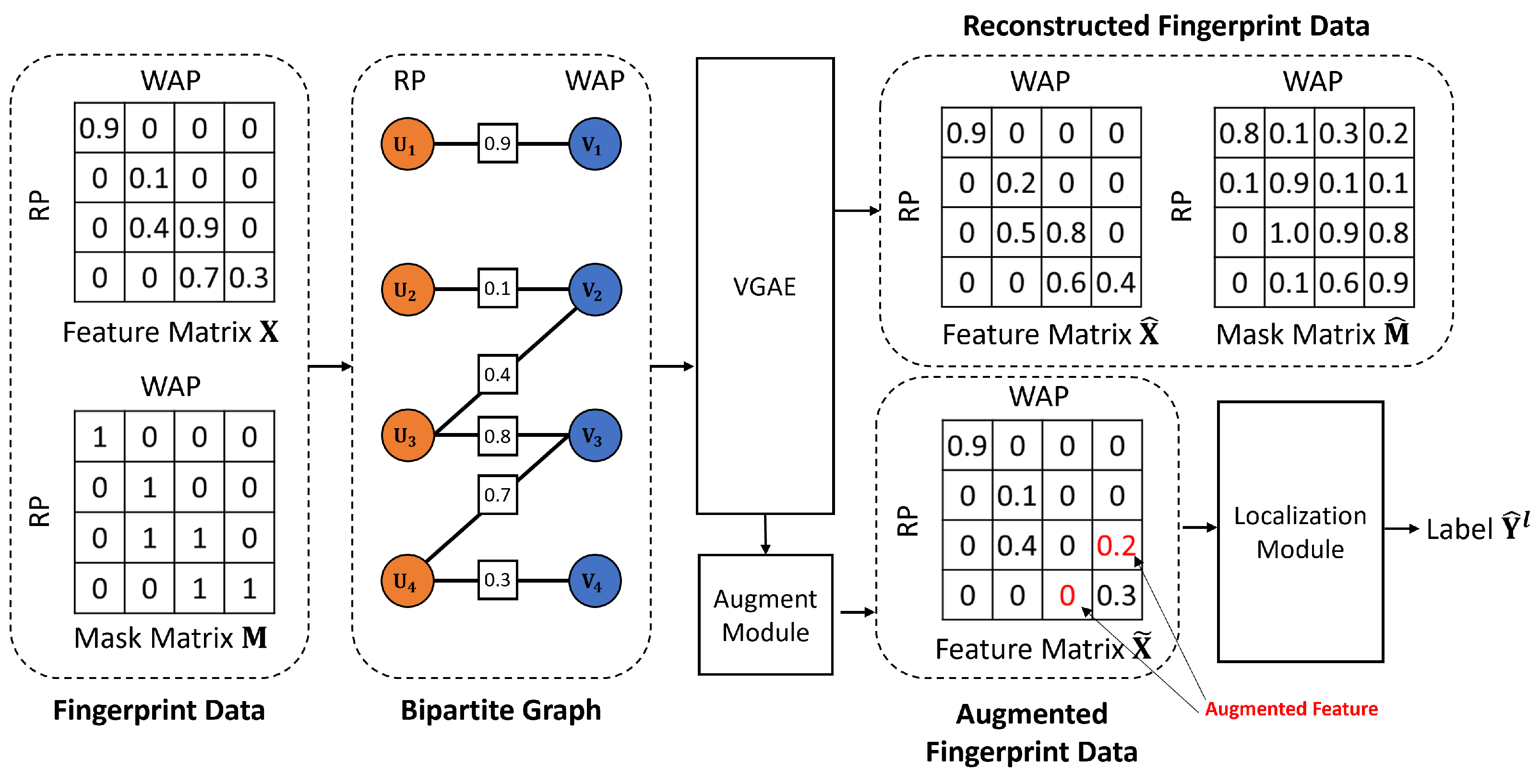
This section details the architecture and components of our proposed framework, FALoc (Feature-level Augmentation for Localization), specifically designed to address the challenge of missing RSSI values in Wi-Fi fingerprint data and thereby enhance indoor localization accuracy. FALoc leverages a graph-based representation of fingerprints, a VGAE to model RSSI observations and values, and a novel augmentation module to generate enriched training data for a neural network-based localization model. An overview of the FALoc framework is presented in Figure 2.

The process begins with the input fingerprint data, consisting of a feature matrix $\mathbf{X}$ (containing normalized RSSI values) and a corresponding binary mask matrix $\mathbf{M}$ (indicating observed RSSI measurements). Due to the inherent sparsity and dynamic nature of real-world Wi-Fi environments, many entries in $\mathbf{X}$ are typically missing, as reflected by zeros in $\mathbf{M}$. To capture the structural relationships within these data, a bipartite graph is constructed where RPs and WAPs form two distinct sets of nodes. An edge exists between an RP and a WAP if an RSSI measurement is observed (i.e., ${\mathbf{M}}_{ik}=1$), with the normalized RSSI value ${\mathbf{X}}_{ik}$ serving as an edge feature.

This graph is then processed by a VGAE, which learns latent embeddings for both RP and WAP nodes. The VGAE aims to reconstruct both the graph structure (i.e., the mask matrix $\widehat{\mathbf{M}}$, representing predicted RSSI observation probabilities) and the edge features (i.e., the RSSI values ${\widehat{\mathbf{e}}}_{ik}$). The encoder part of the VGAE utilizes graph attention mechanisms to aggregate neighborhood information effectively. The augmentation module subsequently leverages the outputs of the VGAE’s decoder ($\widehat{\mathbf{M}}$ and ${\widehat{\mathbf{e}}}_{ik}$) to stochastically generate augmented fingerprint data $\tilde{\mathbf{X}}$. This involves deciding whether to preserve an existing RSSI value, impute a missing one using ${\widehat{\mathbf{e}}}_{ik}$ if ${\widehat{\mathbf{M}}}_{ik}$ suggests a high likelihood of existence, or potentially remove an existing but seemingly unreliable observation. Finally, the augmented fingerprint data $\tilde{\mathbf{X}}$ serves as input to a localization module, typically a neural network, which is trained to estimate the location labels ${\widehat{\mathbf{Y}}}^l$. By training on these enriched and more complete fingerprints, the localization model is expected to achieve improved robustness and accuracy, particularly in scenarios with sparse or missing measurements.

2.1. Bipartite Graph Representation of Wi-Fi Fingerprints

The foundation of FALoc is the representation of Wi-Fi fingerprint data as a bipartite graph, which naturally models the interactions between two distinct types of entities: RPs and WAPs. The bipartite graph structure is known to effectively capture the underlying relationships in highly sparse and irregular wireless signal environments, as it enables expressive graph-based latent representations [29]. The dataset, comprising RSSI measurements from $N_{ap}$ WAPs at $N_{rp}$ RPs, is initially represented by a feature matrix $\mathbf{X}\in {\mathbb{R}}^{N_{rp}\times N_{ap}}$ and an observation mask matrix $\mathbf{M}\in {\{0,1\}}^{N_{rp}\times N_{ap}}$. Each element ${\mathbf{M}}_{ik}$ in $\mathbf{M}$ indicates the presence (1) or absence (0) of an RSSI measurement from the k-th WAP at the i-th RP. The corresponding normalized RSSI value ${\mathbf{X}}_{ik}$ is defined as follows:

$${\mathbf{X}}_{ik}=\left\{\begin{array}{cc}{\displaystyle \frac{r_{ik}-r_{min}}{r_{max}-r_{min}}}\hfill & \mathrm{if}{\mathbf{M}}_{ik}=1,\hfill \\ 0\hfill & \mathrm{if}{\mathbf{M}}_{ik}=0\hfill \end{array}\right.$$

(2)

In Equation (2), $r_{ik}$ is the raw RSSI value from the k-th WAP at the i-th RP, and $r_{min}$ and $r_{max}$ are the minimum and maximum RSSI values observed in the entire dataset, used for scaling. Each RP is associated with three types of location labels: its building identifier, floor level, and specific coordinates (longitude, latitude). These are encoded as one-hot vector ${\mathbf{Y}}_i^b$ for building, ${\mathbf{Y}}_i^f$ for floor, and min–max normalized coordinate pairs ${\mathbf{Y}}_i^l$ for location.

The bipartite graph $\mathcal{G}=(\mathcal{U},\mathcal{V},\mathcal{E})$ is then constructed, where $\mathcal{U}={\left\{u_i\right\}}_{i=1}^{N_{rp}}$ represents the set of RP nodes and $\mathcal{V}={\left\{v_k\right\}}_{k=1}^{N_{ap}}$ represents the set of WAP nodes. An edge $(u_i,v_k)\in \mathcal{E}$ exists if and only if ${\mathbf{M}}_{ik}=1$. The initial features for RP nodes, ${\mathbf{U}}_i^{\left(0\right)}\in {\mathbb{R}}^D$, are derived from their location labels, aiming to provide the model with prior spatial information as follows:

$${\mathbf{U}}_i^{\left(0\right)}={\left({\mathbf{Y}}_i^b\right)}^T\mathbf{B}+{\left({\mathbf{Y}}_i^f\right)}^T\mathbf{F}+{\left({\mathbf{Y}}_i^l\right)}^T{\mathbf{W}}^l$$

(3)

In Equation (3), $\mathbf{B}\in {\mathbb{R}}^{N_b\times D}$, $\mathbf{F}\in {\mathbb{R}}^{N_f\times D}$, and ${\mathbf{W}}^l\in {\mathbb{R}}^{2\times D}$ are trainable embedding matrices for building, floor, and location coordinates, respectively, and D is the dimension of the initial node features. WAP nodes $v_k$ are initialized with trainable feature vectors ${\mathbf{V}}_k^{\left(0\right)}\in {\mathbb{R}}^D$, forming an embedding matrix ${\mathbf{V}}^{\left(0\right)}\in {\mathbb{R}}^{N_{ap}\times D}$. Each edge $(u_i,v_k)$ in $\mathcal{E}$ carries a feature vector ${\mathbf{e}}_{ik}=\left[{\mathbf{X}}_{ik}\right]$, where the scalar ${\mathbf{X}}_{ik}$ is converted into a 1D vector, representing the normalized RSSI value connecting the RP and WAP.

2.2. Variational Graph Auto-Encoder

To learn meaningful representations from the potentially sparse and incomplete fingerprint graph, we employ a VGAE [28]. The VGAE is well-suited for this task due to its ability to learn probabilistic latent embeddings for nodes and its generative nature, which allows for the reconstruction of graph structure (RSSI observation likelihoods) and features (RSSI values). VAE-based models have been shown to be effective in similar scenarios involving fluctuating communication data, demonstrating their suitability for such modeling tasks [30]. It is trained using a self-supervised learning paradigm. The VGAE takes the bipartite graph $\mathcal{G}$ as input and outputs a reconstructed graph $\widehat{\mathcal{G}}$, comprising reconstructed edge existence probabilities and edge features.

2.2.1. Node Embedding Modules and Modified GAT

The core of our VGAE’s encoder lies in its node embedding modules, which update RP and WAP node representations iteratively using a modified graph attention network (GAT) layer [31]. This modified GAT layer is designed to incorporate information from both node features and edge features effectively. We describe the layer using the RP node embedding module as an example. For each layer l, the modified GAT layer processes the node embeddings from the previous layer (${\mathbf{U}}^{(l-1)}$ for RPs, ${\mathbf{V}}^{(l-1)}$ for WAPs) along with the edge features ${\mathbf{e}}_{ik}$ for each connected pair $(u_i,v_k)\in \mathcal{E}$. This module produces the current layer’s RP embeddings (${\mathbf{U}}^{\left(l\right)}$). The attention mechanism utilizes trainable weight matrices (${\mathbf{W}}_u^{\left(l\right)}$, ${\mathbf{W}}_v^{\left(l\right)}$, ${\mathbf{W}}_e^{\left(l\right)}$) and attention vectors (${\mathbf{a}}_u^{\left(l\right)}$, ${\mathbf{a}}_v^{\left(l\right)}$, ${\mathbf{a}}_e^{\left(l\right)}$).

The attention coefficient ${\alpha }_{i,k}^{\left(l\right)}$ between the i-th RP node $u_i$ and its neighboring k-th WAP node $v_k$ in layer l is computed as follows:

$$\begin{array}{cc}\hfill {\widehat{\alpha }}_{i,k}^{\left(l\right)}=& {\left({\mathbf{a}}_u^{\left(l\right)}\right)}^T{\mathbf{W}}_u^{\left(l\right)}{\mathbf{U}}_i^{(l-1)}+{\left({\mathbf{a}}_v^{\left(l\right)}\right)}^T{\mathbf{W}}_v^{\left(l\right)}{\mathbf{V}}_k^{(l-1)}\hfill \\ \hfill & +{\left({\mathbf{a}}_e^{\left(l\right)}\right)}^T{\mathbf{W}}_e^{\left(l\right)}{\mathbf{e}}_{ik}\hfill \end{array}$$

(4)

$${\alpha }_{i,k}^{\left(l\right)}={\displaystyle \frac{exp\left({\sigma }^{\prime }\left({\widehat{\alpha }}_{i,k}^{\left(l\right)}\right)\right)}{{\sum }_{k\in {\mathcal{N}}_i}exp\left({\sigma }^{\prime }\left({\widehat{\alpha }}_{i,k}^{\left(l\right)}\right)\right)+exp\left({\sigma }^{\prime }\left({\widehat{\alpha }}_{i,i}^{\left(l\right)}\right)\right)}}$$

(5)

In Equations (4) and (5), ${\mathcal{N}}_i$ denotes the set of WAP neighbors of the i-th RP node, ${\sigma }^{\prime }$ is the LeakyReLU activation function (with a negative slope of 0.2), and ${\widehat{\alpha }}_{i,i}^{\left(l\right)}$ represents a self-attention component (implicitly defined by the formulation, often involving only the RP node’s own features). The updated embedding ${\mathbf{U}}_i^{\left(l\right)}$ for the i-th RP node is then computed as a weighted sum of transformations of its own features and its neighbors’ features as follows:

$$\begin{array}{c}\hfill {\mathbf{U}}_i^{\left(l\right)}={\alpha }_{i,i}^{\left(l\right)}{\mathbf{W}}_u^{\left(l\right)}{\mathbf{U}}_i^{(l-1)}+\sum _{k\in {\mathcal{N}}_i}{\alpha }_{i,k}^{\left(l\right)}{\mathbf{W}}_v^{\left(l\right)}{\mathbf{V}}_k^{(l-1)}\end{array}$$

(6)

The WAP node embeddings ${\mathbf{V}}^{\left(l\right)}$ are updated through a symmetric process, attending to their neighboring RP nodes.

2.2.2. Encoder Architecture

The encoder of our VGAE consists of a two-layer Graph Neural Network (GNN) architecture. The first GNN layer comprises separate embedding modules (as described above) for RP and WAP nodes. These modules take the initial node features (${\mathbf{U}}^{\left(0\right)}$, ${\mathbf{V}}^{\left(0\right)}$) and the original set of edge features ($\left\{{\mathbf{e}}_{ik}\right\}$) as input, producing updated first-layer embeddings ${\mathbf{U}}^{\left(1\right)}$ and ${\mathbf{V}}^{\left(1\right)}$.

The second GNN layer processes the activated embeddings from the first layer (e.g., after applying an ReLU activation function, $\sigma (·)$). Similarly to the first layer, it contains distinct embedding modules for RP and WAP nodes. These modules operate on $\sigma \left({\mathbf{U}}^{\left(1\right)}\right)$, $\sigma \left({\mathbf{V}}^{\left(1\right)}\right)$, and the set of edge features $\left\{{\mathbf{e}}_{ik}\right\}$. This layer outputs parameters for the probabilistic latent embeddings: the means (${\mathit{\mu }}^{rp}$, ${\mathit{\mu }}^{wap}$) and the logarithms of the standard deviations ($log{\sigma }^{rp}$, $log{\sigma }^{wap}$) for RP and WAP nodes, respectively.

Finally, the encoder utilizes the reparameterization trick to sample the latent node embeddings ${\mathbf{Z}}^{rp}$ and ${\mathbf{Z}}^{wap}$ from the learned distributions:

$${\mathbf{Z}}^{rp}={\mathit{\mu }}^{rp}+\mathit{ϵ}\odot {\mathit{\sigma }}^{rp},{\mathbf{Z}}^{wap}={\mathit{\mu }}^{wap}+\mathit{ϵ}\odot {\mathit{\sigma }}^{wap}$$

(7)

In Equation (7), $\mathit{ϵ}$ is a vector of random samples drawn from a standard normal distribution $\mathcal{N}(0,\mathbf{I})$, and ⊙ denotes element-wise multiplication. These latent embeddings capture the essential characteristics of RPs and WAPs in a lower-dimensional space.

2.2.3. Decoder

The decoder part of the VGAE uses the latent embeddings ${\mathbf{Z}}^{rp}$ and ${\mathbf{Z}}^{wap}$ to reconstruct the original graph properties: the mask matrix $\mathbf{M}$ (predicting the likelihood of an RSSI observation between an RP-WAP pair) and the set of edge features $\left\{{\mathbf{e}}_{ik}\right\}$ (predicting the RSSI values themselves).

For reconstructing the mask matrix, indicating the probability of an edge (RSSI observation), a bilinear decoder is employed. This choice is common for link prediction tasks as it efficiently models pairwise interactions. The reconstructed mask matrix $\widehat{\mathbf{M}}$ is as follows:

$$\widehat{\mathbf{M}}=\mathrm{sigmoid}\left({\mathbf{Z}}^{rp}{\mathbf{W}}^m{\left({\mathbf{Z}}^{wap}\right)}^T\right)$$

(8)

In Equation (8), ${\mathbf{W}}^m$ is a trainable weight matrix. Each entry ${\widehat{\mathbf{M}}}_{ik}$ represents the predicted probability that an RSSI value is observed between the i-th RP and the k-th WAP.

For edge feature reconstruction (predicting RSSI values), a Multi-Layer Perceptron (MLP) decoder is used, offering flexibility to model complex relationships. The reconstructed edge feature (RSSI value) ${\widehat{\mathbf{e}}}_{ik}$ for a potential or existing edge $(u_i,v_k)$ is computed as follows:

$${\widehat{\mathbf{e}}}_{ik}=|{\mathbf{Z}}_i^{rp}-{\mathbf{Z}}_k^{wap}|{\mathbf{W}}^{ef}+{\mathbf{b}}^{ef}$$

(9)

In Equation (9), ${\mathbf{W}}^{ef}$ and ${\mathbf{b}}^{ef}$ are the trainable weight and bias parameters for this edge feature reconstruction network. The output ${\widehat{\mathbf{e}}}_{ik}$ is the predicted normalized RSSI vector.

2.3. Augmentation Module

A key innovation of FALoc is its augmentation module, which leverages the VGAE’s outputs ($\widehat{\mathbf{M}}$ and ${\widehat{\mathbf{e}}}_{ik}$) to generate augmented versions of the fingerprint data. This module aims to create more complete and robust training samples by stochastically imputing likely missing RSSI values or removing potentially spurious ones. The decoder’s output ${\widehat{\mathbf{M}}}_{ik}$ serves as the predicted probability of an RSSI observation between the i-th RP and k-th WAP.

The augmentation logic is based on comparing the original observation mask ${\mathbf{M}}_{ik}$ with the VGAE’s predicted probability ${\widehat{\mathbf{M}}}_{ik}$:

• If ${\mathbf{M}}_{ik}=1$ (observed) and ${\widehat{\mathbf{M}}}_{ik}$ is high (e.g., ${\widehat{\mathbf{M}}}_{ik}$$\ge \alpha$, where $\alpha$ is a predefined threshold), the original RSSI is likely valid and should be preserved with high probability.
• If ${\mathbf{M}}_{ik}=0$ (missing) and ${\widehat{\mathbf{M}}}_{ik}$ is low (e.g., ${\widehat{\mathbf{M}}}_{ik}$$<\alpha$), the absence of RSSI is likely genuine, and it should remain missing with high probability.
• If ${\mathbf{M}}_{ik}=1$ (observed) but ${\widehat{\mathbf{M}}}_{ik}$ is low (e.g., ${\widehat{\mathbf{M}}}_{ik}$$<\alpha$), the observed RSSI might be an outlier or unreliable. This suggests potential feature deletion.
• If ${\mathbf{M}}_{ik}=0$ (missing) but ${\widehat{\mathbf{M}}}_{ik}$ is high (e.g., ${\widehat{\mathbf{M}}}_{ik}$$\ge \alpha$), the original RSSI was likely missing, not genuinely absent. This suggests potential feature imputation using ${\widehat{\mathbf{e}}}_{ik}$.

To implement this stochastic imputation and deletion, we first define a probability ${\mathbf{P}}_{ik}$ for the existence of an augmented link ${\tilde{\mathbf{M}}}_{ik}$ as follows:

$${\mathbf{P}}_{ik}=\left\{\begin{array}{cc}{\displaystyle \frac{{\mathbf{M}}_{ik}+{\widehat{\mathbf{M}}}_{ik}}{2}},\hfill & \mathrm{if}{\widehat{\mathbf{M}}}_{ik}\ge \alpha \hfill \\ 0,\hfill & \mathrm{otherwise}\hfill \end{array}\right.$$

(10)

The augmented mask entry ${\tilde{\mathbf{M}}}_{ik}$ is then sampled from a Bernoulli distribution with probability ${\mathbf{P}}_{ik}$. To enable end-to-end training through this discrete sampling process, we use the Gumbel–softmax reparameterization trick [32] as follows:

$${\tilde{\mathbf{M}}}_{ik}={\displaystyle \frac{1}{1+exp\left(-(log\left({\mathbf{P}}_{ik}\right)+G)/\tau \right)}}$$

(11)

In Equation (11), G is a sample drawn from the $Gumbel(0,1)$ distribution, and $\tau$ is the temperature parameter of the Gumbel–softmax, controlling the smoothness of the approximation. ${\tilde{\mathbf{M}}}_{ik}\approx 1$ indicates the presence of an RSSI value in the augmented fingerprint, and ${\tilde{\mathbf{M}}}_{ik}\approx 0$ indicates its absence.

Finally, the augmented feature matrix $\tilde{\mathbf{X}}$ is constructed based on the original features $\mathbf{X}$, the VGAE-reconstructed features $\widehat{\mathbf{e}}$, and the sampled augmented mask $\tilde{\mathbf{M}}$ as follows:

$${\tilde{\mathbf{X}}}_{ik}=\left\{\begin{array}{cc}{\widehat{\mathbf{e}}}_{ik},\hfill & \mathrm{if}{\tilde{\mathbf{M}}}_{ik}=1\mathrm{and}{\mathbf{M}}_{ik}=0\left(\mathrm{Imputation}\right)\hfill \\ 0,\hfill & \mathrm{if}{\tilde{\mathbf{M}}}_{ik}=0\mathrm{and}{\mathbf{M}}_{ik}=1\left(\mathrm{Deletion}\right)\hfill \\ {\mathbf{X}}_{ik},\hfill & \mathrm{if}{\tilde{\mathbf{M}}}_{ik}=1\mathrm{and}{\mathbf{M}}_{ik}=1\left(\mathrm{Preservation}\right)\hfill \\ 0,\hfill & \mathrm{if}{\tilde{\mathbf{M}}}_{ik}=0\mathrm{and}{\mathbf{M}}_{ik}=0(\mathrm{Remains}\mathrm{absent})\hfill \end{array}\right.$$

(12)

This process generates augmented fingerprints where missing values are probabilistically imputed and unreliable existing values are potentially removed, leading to a richer and more robust training set.

2.4. Localization Module

The localization module is responsible for predicting the user’s location based on the (augmented) Wi-Fi fingerprints. We employ a standard neural network architecture for this task, formulated as follows.

$${\widehat{\mathbf{Y}}}_i^l=F_{\theta }\left({\tilde{\mathbf{X}}}_i\right)$$

(13)

In Equation (13), ${\tilde{\mathbf{X}}}_i$ is the i-th row of the augmented feature matrix (the fingerprint for the i-th RP), $F_{\theta }$ denotes the localization neural network with trainable parameters $\theta$, and ${\widehat{\mathbf{Y}}}_i^l$ represents the estimated location labels (e.g., coordinates) for the i-th RP. The network $F_{\theta }$ is typically an MLP, chosen for its ability to model complex non-linear mappings. The model is trained to minimize an estimation loss (e.g., Mean Absolute Error or Mean Squared Error) between the true labels ${\mathbf{Y}}_i^l$ and the predicted labels ${\widehat{\mathbf{Y}}}_i^l$. By training this module with the augmented data $\tilde{\mathbf{X}}$, we aim to improve its generalization capability, especially its robustness to missing RSSI values encountered during online localization.

2.5. Model Training and Inference

The training of the FALoc framework is performed in two main stages to ensure stability and effective learning. The procedure for training and inference is shown in Algorithm 1.

Algorithm 1 FALoc Training and Inference Procedure

Require: Training data ${\mathcal{D}}_{\mathrm{train}}=\left\{(\mathbf{X},\mathbf{M},\mathbf{Y})\right\}$, learning rates ${\eta }_1$, ${\eta }_2$, balance weight $\lambda$ Ensure: Trained localization model $F_{\theta }$   Pretraining (VGAE only):   for each epoch do      Apply edge dropout to graph E      Reconstruct $\widehat{\mathbf{M}},\widehat{\mathbf{X}}$ via VGAE      Compute loss ${\mathcal{L}}_{\mathrm{pre}}={\mathcal{L}}_M+{\mathcal{L}}_X$      Update VGAE with learning rate ${\eta }_1$   end for   Main Training (End-to-End):   for each epoch do      Generate augmented data using Gumbel-softmax      Predict $\widehat{\mathbf{Y}}=F_{\theta }\left(\mathrm{augmented}\mathrm{data}\right)$      Compute loss ${\mathcal{L}}_{\mathrm{main}}={\mathcal{L}}_M+{\mathcal{L}}_X+\lambda {\mathcal{L}}_Y$      Update all modules with learning rate ${\eta }_2$      Apply early stopping if validation degrades   end for   Inference:   Given query ${\mathbf{x}}_{\mathrm{query}}$, return ${\widehat{\mathbf{y}}}_{\mathrm{query}}=F_{\theta }\left({\mathbf{x}}_{\mathrm{query}}\right)$

Pretraining Phase: Initially, only the VGAE component is pretrained. The objective during this phase is to enable the VGAE to accurately learn to reconstruct the graph structure (mask matrix $\mathbf{M}$) and the edge features (RSSI values $\mathbf{X}$). The loss function for pretraining is as follows.

$${\mathcal{L}}_{pretrain}={\mathcal{L}}_M(\mathbf{M},\widehat{\mathbf{M}})+{\mathcal{L}}_X(\mathbf{X},\widehat{\mathbf{X}})$$

(14)

In Equation (14), ${\mathcal{L}}_M(\mathbf{M},\widehat{\mathbf{M}})$ is the binary cross-entropy reconstruction loss for the mask matrix, encouraging $\widehat{\mathbf{M}}$ to predict true observation likelihoods. ${\mathcal{L}}_X(\mathbf{X},\widehat{\mathbf{X}})$ is the reconstruction loss for the feature matrix, typically the Mean Absolute Error (MAE) calculated only over observed entries (where ${\mathbf{M}}_{ik}=1$), penalizing deviations between original and reconstructed RSSI values. To enhance generalization during VGAE training and prevent the model from simply memorizing the input graph, edge dropout is applied: a certain percentage of edges from $\mathcal{E}$ are randomly removed before being fed into the VGAE at each training epoch.

Main Training Phase (End-to-End): After pretraining the VGAE, the entire FALoc framework, including the VGAE, the augmentation module, and the localization module, is trained end-to-end. The overall loss function in this phase incorporates the VGAE reconstruction losses and the localization task loss as follows:

$${\mathcal{L}}_{main}={\mathcal{L}}_M(\mathbf{M},\widehat{\mathbf{M}})+{\mathcal{L}}_X(\mathbf{X},\widehat{\mathbf{X}})+\lambda {\mathcal{L}}_Y({\mathbf{Y}}^l,{\widehat{\mathbf{Y}}}^l)$$

(15)

In Equation (15), ${\mathcal{L}}_Y({\mathbf{Y}}^l,{\widehat{\mathbf{Y}}}^l)$ is the loss for the location label prediction (e.g., MAE for coordinates), and $\lambda$ is a hyperparameter balancing the reconstruction tasks with the primary localization task. During this phase, the gradients from the localization loss ${\mathcal{L}}_Y$ flow back through the augmentation module (enabled by the Gumbel–softmax trick) and into the VGAE, allowing the VGAE to learn representations that are not only good for reconstruction but also beneficial for the downstream localization task. Early stopping is employed based on the localization performance on a validation set to prevent overfitting.

Inference Phase: During the online location inference phase, the system processes a new Wi-Fi fingerprint observed by the user’s device to estimate their current location. Unlike the training phase where data augmentation is crucial, the inference phase in FALoc is straightforward. The raw fingerprint vector ${\mathbf{x}}_{query}$, as collected from the environment (which may contain missing RSSI values), is directly fed as input to the trained localization module $F_{\theta }$. The localization network then outputs the predicted location labels ${\widehat{\mathbf{Y}}}_{query}^l$ as follows:

$${\widehat{\mathbf{Y}}}_{query}^l=F_{\theta }\left({\mathbf{x}}_{query}\right)$$

(16)

The rationale behind this direct approach is that the localization module $F_{\theta }$ has already been trained on a diverse set of augmented fingerprints generated by the VGAE and augmentation module. This comprehensive training is intended to equip $F_{\theta }$ with the robustness to effectively handle incomplete or varied fingerprint data encountered during real-world inference, without requiring explicit data augmentation or completion steps at inference time.

3. Performance Evaluation

To assess the effectiveness of the proposed FALoc framework, we conducted comprehensive experiments using a well-established public benchmark dataset. This section details the dataset, evaluation metrics, experimental setup, and a comparative analysis of the results.

3.1. Dataset Description

We utilized the UJIIndoorLoc dataset [27] and the UTSIndoorLoc dataset [16], which are large-scale benchmarks for Wi-Fi fingerprinting-based indoor localization. The UJIIndoorLoc dataset was collected from three multi-floor buildings at Jaume I University, covering approximately 108,703 m². It includes RSSI measurements from 520 distinct WAPs and provides additional metadata such as FLOOR, BUILDINGID, SPACEID, RELATIVEPOSITION, USERID, PHONEID, TIMESTAMP, LONGITUDE, and LATITUDE. The UTSIndoorLoc dataset was collected in a multi-floor building at the University of Technology Sydney. Each sample consists of a 589-dimensional RSSI vector along with metadata including Pos_x, Pos_y, Floor_ID, Building_ID, User_ID, Phone_type, and Time.

The distribution of observed RSSI values spans from −104 dBm to 0 dBm in the UJIIndoorLoc dataset, and from −96 dBm to −37 dBm in the UTSIndoorLoc dataset. In UJIIndoorLoc and UTSIndoorLoc dataset, RSSI values that were not observed at a given location are marked with +100 dBm. We used these +100 dBm entries to identify unobserved signals, setting the corresponding elements in our mask matrix $\mathbf{M}$ to 0 (i.e., ${\mathbf{M}}_{ik}=0$). Subsequently, for the feature matrix $\mathbf{X}$ used as model input, these unobserved signals were represented by a normalized value of 0, following Equation (2) in Section 2.1. This process results in fingerprint vectors that are often incomplete. The UJIIndoorLoc and UTSIndoorLoc datasets exhibit considerable variation in observed WAPs and RSSI values, making it a suitable testbed for evaluating FALoc, which is designed to handle such incomplete data.

3.2. Evaluation Metrics and Baselines

The primary performance metric used for evaluating localization accuracy is the mean Euclidean distance error, calculated between the predicted 2D coordinates (longitude and latitude) and the ground truth coordinates of the test samples. In addition to the mean error, we report several other statistical metrics to provide a comprehensive understanding of the error distribution: MAE, Mean Squared Error (MSE), Root Mean Square Error (RMSE), and the coefficient of determination ($R^2$). Lower values for mean error, MAE, MSE, and RMSE indicate better performance, while a higher $R^2$ value signifies a better fit of the model to the data.

Our proposed method, MLP with FALoc, involves training an MLP-based localization module using the augmented fingerprints generated by FALoc as described in Section 3. As a baseline for comparison, we implemented a standard MLP without FALoc. For this baseline, the MLP was trained directly on the original fingerprint data, where missing RSSI values (identified from the +100 dBm markers and subsequently masked in $\mathbf{M}$) were represented as 0 after the same normalization process applied to FALoc’s input. This zero-filling approach is a common practice for handling missing data when no specialized mechanism is employed. This ensures a fair comparison, isolating the impact of the FALoc feature augmentation and imputation strategy. In addition to the zero-filled baseline, we also implemented a variant of FALoc using a traditional variational autoencoder (VAE) instead of the proposed VGAE, in order to assess the benefits of graph-based modeling. This VAE-based model was trained under the same augmentation and MLP pipeline, but without exploiting the graph structure of the fingerprints. While our framework also processes building and floor labels as part of the RP node features in the VGAE, the quantitative evaluation presented in this section focuses on the accuracy of 2D coordinate prediction, which is the most common primary metric for these dataset.

3.3. Experimental Setup

The UJIIndoorLoc and UTSIndoorLoc datasets was divided into a training set and a testing set. The training samples were further partitioned, with 80% used for actual model training and 20% reserved as a validation set. This validation set was used for hyperparameter tuning and to implement an early stopping mechanism to prevent overfitting. Early stopping was triggered if the localization error on the validation set did not show improvement for a patience period.

A MLP served as the core architecture for the localization module ($F_{\theta }$) in both the FALoc-enhanced setup and the baseline. We implemented FALoc and the baseline MLP model using PyTorch 2.6.0 and PyTorch Geometric hl2.4.0 libraries. To ensure optimal performance for both configurations, an extensive grid search was conducted to find the best hyperparameters for the MLP models and for the FALoc-specific components (e.g., VGAE architecture, $\alpha$, $\tau$). The optimized hyperparameters used for the final evaluation are detailed in

Table 1. Hyperparameters used for evaluation.

Parameter	Value
D (Initial node feature dim.)	256
VGAE Encoder Arch. (GAT layers)	First, Layer (256 → 128), Mean & Log Std. (128 → 64)
VGAE Latent Dim. ($D_z$)	64
VGAE Decoder Arch. (Mask)	Bilinear ($64\times 64$)
VGAE Decoder Arch. (RSSI)	Linear ($64\to 1$)
VAE Input Dim.	1040 (RSSI: 520 + Mask: 520)
VAE Encoder Arch.	1040 → 512 → 256 → 128
VAE Decoder Arch.	128 → 256 → 512 → 1040
$\alpha$ (Augmentation threshold)	0.96
$\tau$ (Gumbel-softmax temp.)	0.05
Localization MLP Arch. ($F_{\theta }$, UJIIndoorLoc)	520 → 500 → 500 → 500 → 500 → 2
Localization MLP Arch. ($F_{\theta }$, UTSIndoorLoc)	589 → 64 → 256 → 128 → 64 → 2
MLP dropout ($F_{\theta }$, UJIIndoorLoc)	0.5
MLP dropout ($F_{\theta }$, UTSIndoorLoc)	0.0
Edge dropout (VGAE training)	0.3
Activation function	ReLU
Optimizer	Adam (lr = 0.001)

.

In Table 1, D represents the dimensionality of the initial RP and WAP node features. The VGAE Encoder Architecture indicates the number of units in successive GAT layers leading to the parameters of the latent distributions; for instance, ’First, Layer(256 → 128), Mean&Log Std.(128 → 64)’ means the initial 256-dimensional features are processed by a GAT layer outputting 128 features, followed by another GAT layer outputting 64 features for both mean and standard deviation vectors, resulting in a latent dimension 64 per node type. The VGAE Decoder for the mask is bilinear, and for RSSI values, it is an MLP. The Localization MLP Architecture ’520 → 500 → 500 → 500 → 500 → 2’ describes an MLP with an input layer (size corresponding to the number of WAPs, 520), four hidden layers each with 500 neurons, and an output layer predicting 2D coordinates.

3.4. Results

Table 2. Positioning error statistics and metrics on UJIIndoorLoc and UTSIndoorLoc datasets.

UJIIndoorLoc Dataset
Method	Mean Error (m)	MAE (m)	MSE (m2)	RMSE (m)	$R^2$
MLP with FALoc (VGAE)	7.135	4.561	49.603	7.043	0.993
MLP with FALoc (VAE)	7.808	4.934	61.878	7.866	0.9978
MLP without FALoc (Baseline)	8.191	5.214	66.294	8.142	0.991
UTSIndoorLoc Dataset
Method	Mean Error (m)	MAE (m)	MSE (m2)	RMSE (m)	$R^2$
MLP with FALoc (VGAE)	7.138	4.232	39.121	6.255	0.722
MLP with FALoc (VAE)	7.382	4.413	40.074	6.330	0.694
MLP without FALoc (Baseline)	7.808	4.819	43.435	6.591	0.605

summarizes the positioning error statistics for both the baseline MLP and the MLP enhanced with our FALoc framework. The corresponding cumulative distribution function (CDF) of positioning errors is illustrated in Figure 3, providing a visual representation of the error distributions across all test samples.

The results clearly demonstrate that integrating FALoc significantly improves the localization performance of the MLP model across both datasets. On the UJIIndoorLoc dataset, the mean positioning error decreased from 8.191 m for the baseline MLP to 7.135 m with FALoc (VGAE), representing a relative improvement of approximately 12.9%. Similarly, the MAE dropped from 5.214 to 4.561 m, while the MSE was reduced from 66.294 to 49.603 ${\mathrm{m}}^2$. The RMSE also improved from 8.142 to 7.043 m, a reduction of about 13.5%. These improvements in squared error metrics suggest that FALoc effectively mitigates large outliers in positioning error, likely by generating more reliable fingerprint representations in place of missing or noisy signals. The $R^2$ value also increased slightly from 0.991 to 0.993, indicating that the model with FALoc better explains the variance in true locations.

On the UTSIndoorLoc dataset, which features a different environment and Wi-Fi topology, a similar trend is observed. The mean positioning error improved from 7.808 m (baseline) to 7.138 m (FALoc-VGAE), and the MAE dropped from 4.819 to 4.232 m. The MSE decreased from 43.435 to 39.121 ${\mathrm{m}}^2$, and RMSE was reduced from 6.591 to 6.255 m. Although the absolute errors on UTSIndoorLoc are lower than those on UJIIndoorLoc, the relative improvements remain consistent, confirming that FALoc generalizes well across different deployment settings. The increase in $R^2$ from 0.605 to 0.722 further supports that FALoc enhances the model’s ability to predict accurate positions even in more challenging or diverse environments.

In addition to outperforming the baseline MLP, the proposed FALoc framework based on VGAE also demonstrates superiority over the prior VAE-based variant across both datasets. On the UJIIndoorLoc dataset, the VGAE model achieved a lower mean error (7.135 m vs. 7.808 m) and MAE (4.561 m vs. 4.934 m) compared to the VAE model. Furthermore, VGAE showed substantial improvements in MSE (49.603 vs. 61.878 ${\mathrm{m}}^2$) and RMSE (7.043 m vs. 7.866 m), indicating its effectiveness in reducing both average and large deviations in localization. Even the $R^2$ score, already high with VAE (0.9978), was slightly better with VGAE (0.993), highlighting consistent model generalization. On the UTSIndoorLoc dataset, which presents a more diverse environment, similar patterns are observed. VGAE outperformed VAE across all metrics: mean error (7.138 m vs. 7.382 m), MAE (4.232 m vs. 4.413 m), MSE (39.121 vs. 40.074 ${\mathrm{m}}^2$), RMSE (6.255 m vs. 6.330 m), and $R^2$ (0.722 vs. 0.694). These results confirm that VGAE-based FALoc not only advances beyond the traditional zero-filled baseline, but also improves upon earlier augmentation techniques, offering more robust and generalizable localization performance across heterogeneous indoor environments.

Figure 3 further corroborates these findings. The CDF curve for the FALoc-enhanced MLP consistently lies above that of the baseline MLP across nearly all error ranges. This is especially pronounced in the lower error region (e.g., 0–10 m), where a notably larger fraction of test samples achieve lower positioning errors when FALoc is employed. For instance, with FALoc, over 75% of the predictions fall within a 10 meter error margin, compared to approximately 65% for the baseline. This upward shift in the CDF curve highlights not only a reduction in average error but also an improvement in the overall reliability and robustness of the localization model.

In summary, the empirical evidence strongly supports the efficacy of FALoc. By explicitly modeling RSSI observation probabilities and performing feature-level data augmentation to handle missing values, FALoc enables the localization model to learn more effectively from incomplete real-world data. This results in statistically and practically significant improvements across all standard performance metrics, leading to more accurate and consistent indoor localization outcomes. The enhanced performance, particularly the reduction in larger errors, can be attributed to FALoc’s ability to provide the localization model with intelligently imputed and more complete feature vectors, mitigating the adverse effects of naively handled (e.g., zero-filled) missing data that the baseline model contends with.

4. Discussion and Future Work

4.1. Feasibility of Real-World Deployment

One important consideration for real-world deployment is the sensitivity of the threshold parameter $\alpha$, which determines the confidence margin used in the neighbor filtering step. As $\alpha$ directly influences the trade-off between recall and precision, its optimal value is not universal but must be adjusted according to the characteristics of the deployment environment, such as signal fluctuation, density of reference points, and physical obstructions. Practitioners should conduct environment-specific calibration to fully leverage the benefits of our framework. Future work could explore adaptive thresholding strategies that dynamically adjust $\alpha$ based on signal statistics based on the feature of datasets.

Another important consideration is the computational complexity. The proposed method utilizes deep learning only during the offline training phase, which is typically conducted on server-side infrastructure, where resource constraints are less critical. In contrast, the online inference phase, which runs on the user device, requires a computational load comparable to that of conventional fingerprinting-based inference methods. Therefore, the proposed framework is sufficiently feasible even on resource-constrained devices and does not impose significant computational overhead during real-time inference. In addition, while the use of graph-based modeling may raise concerns regarding scalability, particularly in large-scale graphs, it is important to note that such operations are confined to the offline training phase. Moreover, in our current datasets, the number of WAPs is around 500, which reflects realistic deployment scenarios and remains well within the capacity of standard training infrastructure. Thus, scalability does not pose a practical limitation in the context of our framework.

To evaluate the real-world feasibility of real-time deployment, we measured the computation time during the online inference phase.

Table 3. Computation time of the proposed method in training and inference phases (in ms).

Dataset	Training Time (ms)	Inference Time (ms)
UJIIndoorLoc	140.0	0.261
UTSIndoorLoc	117.0	0.226

presents the computation times of both baseline methods and the proposed approach. As shown in Table 3, the inference time of our method is significantly lower than that of conventional WKNN-based techniques [13], which typically operate in the tens of milliseconds, thereby demonstrating strong potential for real-time application even under strict latency constraints.

4.2. Future Work

While FALoc demonstrates promising results, we acknowledge certain areas for future exploration. For instance, the current VGAE architecture and augmentation policy, though effective, might benefit from further optimization for even greater efficiency or adaptability to different types of missingness.

Building upon this work, our future research will focus on several key directions. We plan to investigate more advanced graph neural network architectures. For instance, recent work has applied self-attention mechanisms to graph learning to improve representational capacity [33]. Following such examples, we intend to explore architectures incorporating temporal dynamics or attention mechanisms tailored for heterogeneous graph structures, to further refine the modeling of RP-WAP interactions.

Additionally, we aim to develop adaptive augmentation policies that can dynamically adjust the imputation and deletion strategy based on data characteristics or even feedback from the localization model during training. In particular, since WiFi signals are highly sensitive to environmental changes, recent studies have explored models that adapt to variations across different data collection domains. For example, some works have focused on improving feature extractors to alleviate domain imbalance [34], while others have enhanced the mapping between signal variations and target locations to achieve robust localization [35]. Exploring the framework’s scalability and performance across a wider range of diverse indoor environments, including those with extremely high levels of data sparsity, also remains a priority.

In the current study, all experiments were conducted using a single benchmark dataset, while this allowed us to verify the effectiveness of the proposed method under controlled conditions, we acknowledge that further evaluation of additional datasets is necessary to validate its generalizability across different domains. However, due to differences in label definitions, feature spaces, and data collection protocols, applying the same experimental setting across multiple datasets was considered out of the current study’s scope. As part of our future work, we plan to expand our evaluation to include multiple datasets collected under varying conditions, which will allow a more comprehensive assessment of domain robustness and practical applicability.

Another important direction for future research is to conduct a detailed ablation study to isolate and quantify the contribution of each component in the proposed framework. The current design was developed as an integrated pipeline, where all components are intended to operate synergistically rather than independently. Therefore, we focused on validating the effectiveness of the full system rather than optimizing individual parts in isolation, while we acknowledge that such synergy may not be fully captured through ablation analysis, we recognize the importance of understanding the internal contribution of each module. A comprehensive ablation study will be considered in future work to further clarify the role of each component in enhancing overall localization performance.

While our proposed method demonstrates promising performance compared to the MLP baseline, it has not yet been benchmarked against other state-of-the-art models such as GAN-based, CNN-based, or RNN-based approaches. This limitation stems from practical constraints in the current study, such as time and scope. Nonetheless, we acknowledge that such comparisons are essential to more rigorously assess the generalizability and competitiveness of the proposed framework. As part of our future work, we plan to conduct extensive comparisons with a broader range of advanced models, including GANs, CNNs, and RNNs, which have shown strong performance in data augmentation and localization tasks. Such benchmarking will provide deeper insights into the strengths and limitations of our method in comparison to alternative architectures and strategies.

5. Conclusions

This paper introduced FALoc, a novel framework for Wi-Fi fingerprinting-based indoor localization, designed to effectively address the critical challenge of missing RSSI values—a common issue that degrades localization accuracy in real-world environments. Our core contribution lies in a feature-level data augmentation technique rooted in a graph-based representation of Wi-Fi fingerprints. By employing a bipartite graph of RPs and WAPs and utilizing a VGAE, FALoc learns to model not only the RSSI values themselves but also their observation probabilities. Our empirical evaluation of the UJIIndoorLoc and UTSIndoorLoc datasets, a benchmark known for its data inconsistencies, validated the effectiveness of FALoc. The framework achieved mean localization errors of 7.137 m (12.9% gain) on UJIIndoorLoc and 7.138 m (8.6% gain) on UTSIndoorLoc, consistently outperforming the MLP baselines. This improvement underscores the practical benefits of directly tackling data incompleteness, potentially leading to more reliable and robust indoor localization systems with reduced susceptibility to dynamic signal environments.