Explainable Face Recognition via Improved Localization

Abstract

Biometric authentication has become one of the most widely used tools in the current technological era to authenticate users and to distinguish between genuine users and impostors. The face is the most common form of biometric modality that has proven effective. Deep learning-based face recognition systems are now commonly used across different domains. However, these systems usually operate like black-box models that do not provide necessary explanations or justifications for their decisions. This is a major disadvantage because users cannot trust such artificial intelligence-based biometric systems and may not feel comfortable using them when clear explanations or justifications are not provided. This paper addresses this problem by applying an efficient method for explainable face recognition systems. We use a Class Activation Mapping (CAM)-based discriminative localization (very narrow/specific localization) technique called Scaled Directed Divergence (SDD) to visually explain the results of deep learning-based face recognition systems. We perform fine localization of the face features relevant to the deep learning model for its prediction/decision. Our experiments show that the SDD Class Activation Map (CAM) highlights the relevant face features very specifically and accurately compared to the traditional CAM. The provided visual explanations with narrow localization of relevant features can ensure much-needed transparency and trust for deep learning-based face recognition systems. We also demonstrate the adaptability of the SDD method by applying it to two different techniques: CAM and Score-CAM.

1. Introduction

Deep learning models have become ubiquitous across a wide range of application domains due to their efficiency and high performance. The field of biometric authentication is also adopting deep learning-based systems such as face, fingerprint, and iris recognition systems. However, in most cases, the results or decisions of these models are not transparent, i.e., it is not clear why a deep learning model achieved a specific prediction. This can lead to a lack of trust in the results. To achieve transparency and increase the trustworthiness of such systems, explainable AI techniques have drawn much attention [1]. Explainability seeks to provide the reason behind the prediction/classification/decision of a deep learning model. There are multiple types of explanation techniques; however, this paper primarily focuses on the visual explanations of deep learning models [2], which is called discriminative localization. Discriminative localization refers to the process of identifying and highlighting specific regions in an image that are most relevant or important for a model’s decision making, particularly for distinguishing between different classes [3].

Explainability can enhance trust in deep learning-based biometric systems such as face recognition. Explaining the predictions of deep learning models is a complicated task, as the structure of a deep learning model is very complex [4]. There are different techniques to visually explain the decision of a deep learning model, such as Saliency Maps [5], LIME [6], Class Activation Mapping (CAM) [3], Gradient-weighted Class Activation Mapping (Grad-CAM) [7], etc.

In this paper, we use a CAM-based discriminative localization technique, Scaled Directed Divergence (SDD) [8], for narrow/specific localization of relevant (relevant to the deep learning model for its prediction/decision) spatial regions of face images. A Class Activation Map (CAM) highlights the class-specific discriminative regions relevant to the deep learning model for arriving at its prediction/decision. The SDD technique is particularly useful for the fine localization of class-specific features in situations of class overlapping. Class overlapping occurs when images from different classes share similar regions or features, making it challenging for a model to distinguish between them. Therefore, the SDD technique is suitable for visually explaining the decisions of face recognition systems, which often deal with similar face images (face images of different individuals that share similar features).

In a previous paper, Williford et al. [9] performed explainable face recognition using a new evaluation protocol called the “Inpainting Game”. Given a set of three images (probe, mate 1, and non-mate), the explainable face recognition algorithm was to identify pixels in a specific region that contribute to the mate’s identity more than to the non-mate’s identity. This identification was represented through a saliency map, indicating the discriminative regions for mate recognition. The “Inpainting Game” protocol was used for the evaluation of the identification made by the explainable face recognition algorithm. However, Williford et al. did not consider a multi-class model for explainable face recognition where there are both similar and non-similar classes. Rajpal et al. [10] used LIME to visually explain the predictions of face recognition models. However, they did not consider the case of class overlap (common areas highlighted in the visual explanations of different classes); therefore, their explanations failed to narrowly show the important features responsible for making a decision.

In this work, we implement the Scaled Directed Divergence (SDD) method to enhance the interpretability of convolutional neural network (CNN) predictions for face recognition tasks. A CNN model is trained on the multi-class FaceScrub dataset [11], and its classification accuracy is evaluated on the test set. For a test image, we identify the predicted class and apply the SDD technique to generate the class activation map (SDD CAM), enabling fine localization of the most relevant spatial regions contributing to the model’s decision. Compared to traditional CAM, the SDD CAM provides more precise and focused explanations. We perform the same experiments with another multi-class dataset, sampled CASIA-WebFace [12]. We evaluate the quality and effectiveness of these visual explanations generated by the SDD method. Additionally, we demonstrate the adaptability of the SDD technique by integrating it with the Score-CAM method [13] to generate SDD Score-CAMs, and we assess their explanatory performance as well. The key contributions of this paper are as follows:

• Applying the SDD method for explainable face recognition;
• Evaluating the visual explanation quality of SDD CAM;
• Demonstrating the integration of SDD with Score-CAM to generate SDD Score-CAM explanations and show the adaptability of the SDD method.

The code is available at https://github.com/rashikshadman/Scaled_Directed_Divergence (accessed on 2 July 2025).

The paper is organized as follows: Section 2 reviews related work; Section 3 presents the methodology and algorithm; Section 4 describes the face recognition model, dataset, experimental setup, and visual explanation results; Section 5 provides the evaluation outcomes; Section 5.3 offers a discussion of the results; Section 6 explores the adaptability of the SDD technique; and Section 7 concludes the paper.

2. Related Work

This section briefly highlights key visual explanation techniques, which are foundational to interpretability in deep learning models.

Saliency Maps [5] prioritize pixels in an image based on their impact on the output score of a CNN. This is achieved through a first-order Taylor expansion to approximate the model’s nonlinear response. The resulting map highlights the most influential pixels, computed via backpropagation. Local Interpretable Model-agnostic Explanations (LIMEs) [6] provide local explanations by approximating a complex model with an interpretable one around a specific prediction. LIME helps demystify why a model made a particular prediction by simplifying the decision process for individual instances.

DeepLIFT [14] decomposes neural network outputs by attributing the prediction to the contributions of input features, comparing activations with a reference. This method performs a comparison efficiently in a single backward pass. Guided Backpropagation [15] improves visualization by combining “deconvnet” and backpropagation, enabling the visualization of important features at both the final and intermediate layers of the network. This technique focuses on preserving positive gradients, making it ideal for understanding what drives activation in the network. Tang et al. [16] present a two-stage meta-learning framework that integrates attention-guided pyramidal features to enhance performance in few-shot fine-grained recognition tasks. The proposed method effectively captures discriminative features at multiple scales, facilitating improved classification accuracy with limited labeled samples.

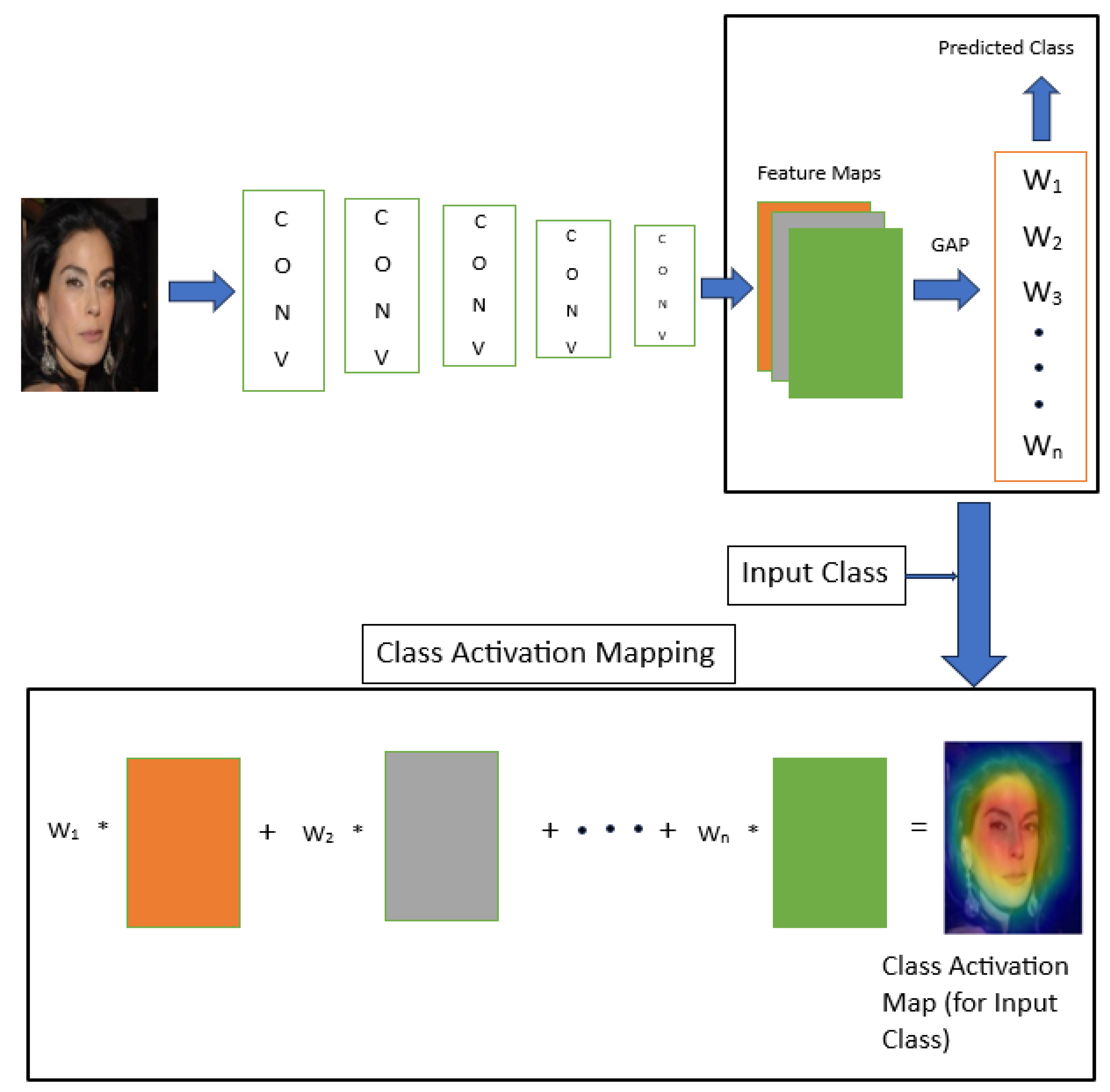
Class Activation Mapping (CAM) [3] highlights discriminative image regions by projecting the weights from the final, fully connected layer onto convolutional feature maps. This technique has been foundational in classifying images and is described in detail in Section 3. The Scaled Directed Divergence (SDD) technique, based on CAM, is used in this work to explain face recognition in Section 4. Gradient-weighted Class Activation Mapping (Grad-CAM) [7] extends CAM by incorporating gradient information, which helps identify important image regions associated with specific classes. Grad-CAM enhances class-specific localization by leveraging gradients from the final convolutional layers. Guided Grad-CAM, which combines Grad-CAM and Guided Backpropagation, offers high-resolution, class-discriminative visualizations.

3. Methodology and Algorithm

In this section, we describe the Class Activation Maps (CAMs) [3] and Scaled Directed Divergence (SDD) [8]. We use the SDD technique for our experiments on visual explainability. The SDD technique uses CAMs and is suitable for scenarios with overlapping classes, which is mentioned in Section 1.

3.1. Class Activation Maps

The main goal of Class Activation Maps (CAMs) is to highlight the regions of an image that are most influential for the decision of a CNN model. CAMs are useful for visually explaining the model’s focus areas.

This approach involves tracing the predicted class score back to the preceding convolutional layer to generate CAMs. These maps serve to accentuate regions in the input image that are specifically relevant to the identified class, showcasing discriminative features.

The last convolutional layer in CNN captures features significant for the prediction of the CNN model. These features are used to generate CAMs for the respective classes. The weighted sum of the feature maps is computed to generate CAMs. The CAM generation procedure is explained in Figure 1.

Following the terminology and notations from Zhou et al. [3], let softmax be the final output layer. For a test image, $f_k(x,y)$ is the activation of unit k at spatial location $(x,y)$ in the last convolutional layer. Then, the global average pooled result $F_k$ for unit k is ${\sum }_{x,y}{f}_k(x,y)$. The input for the softmax ($S_c$) for the target class c is ${\sum }_k{w}_k^c{F}_k$. The target class refers to the specific class label for which the model’s attention or activation map is generated, highlighting the image regions that contribute most to the model’s prediction of that class. Here, $w_k^c$ represents the weight corresponding to class c for unit k. Basically, the significance of $F_k$ for class c is recognized by $w_k^c$. From $F_k={\sum }_{x,y}{f}_k(x,y)$, the class score $S_c$ can be written as follows [3]:

$$S_c=\sum _k{w}_k^c\sum _{x,y}{f}_k(x,y)=\sum _{x,y}\sum _k{w}_k^c{f}_k(x,y).$$

(1)

The CAM $M_c$ for class c is [3]

$$M_c(x,y)=\sum _k{w}_k^c{f}_k(x,y).$$

(2)

Here, $M_c(x,y)$ is the spatial element at grid $(x,y)$.

3.2. Scaled Directed Divergence (SDD)

Scaled Directed Divergence (SDD) [8] is a visual explainability technique based on CAMs. This technique is useful for the narrow/specific localization of relevant features (important to the CNN model for its prediction) of an input image compared to traditional CAMs.

Considering a multi-class model of $i+1$ classes, let $S=\{x_o,\dots \dots ,x_i\}$ be the set of CAMs. Let $T\left(t\right)=S\backslash \left\{x_t\right\}$ be the set of CAMs where the target class (the class for which SDD CAM is generated) CAM $x_t$ is removed from set S. Then, the SDD CAM for target class t is defined as follows [8]:

$$CA{M}_{SDD}^t=e^{\alpha (x_{t}F-{\sum }_{kϵT\left(t\right)}{x}_k)}.$$

(3)

We have improved the SDD technique by updating the scaling factor F and parameter $\alpha$. The target class CAM is scaled by F (where F = $\left|S\right|$ ∗ (average mean absolute value of all CAMs except target class CAM / mean absolute value of target class CAM); the minimum value of F is S and the maximum value is 50) before computing the divergence values between the target CAM and other CAMs. Parameter $\alpha$ (where $\alpha =0.2+(stddev\left(CA{M}_{SDD}\right)/(stddev\left(CA{M}_{SDD}\right)+1))\ast 0.2$) amplifies or decreases the divergence values to be exponentiated. The set of CAMs S only needs to contain the target CAM and CAMs with significant overlap. An overview of the SDD technique is shown in Figure 2.

4. Explainable Face Recognition

Our experiment is divided into two parts: (1) using SDD for explaining the face recognition model’s results, and (2) evaluation of SDD results. We first describe two face recognition models and use SDD to visually explain their results (Section 4.1 and Section 4.2).

4.1. Face Recognition Model—1

We use the state-of-the-art AdaFace model [17] for face recognition. The AdaFace model is ResNet100, which is pre-trained on the WebFace12M [18] face dataset. For the face classification task, the pre-trained AdaFace model is fine-tuned on the FaceScrub dataset [11] (a public dataset). The FaceScrub dataset is a high-quality resource for face recognition research, offering several advantages in terms of diversity and data integrity:

• Extensive Coverage: Comprising 43,148 face images of 530 celebrities (265 male and 265 female), FaceScrub provides a substantial number of images per individual. This extensive coverage enhances the dataset’s utility for training and evaluating face recognition models.
• Diverse Real-World Data: The images were collected from various online sources, including news outlets and entertainment websites, capturing subjects in uncontrolled environments. This diversity introduces variations in pose, lighting, and expression, which are crucial for developing robust face recognition systems.
• Rigorous Data Cleaning Process: To ensure data quality, FaceScrub employs an automated cleaning approach that detects and removes irrelevant or mislabeled images. This process is complemented by manual verification, resulting in a dataset that is both large and accurate.

These attributes make FaceScrub a valuable dataset for advancing face recognition technologies, providing researchers with a rich and diverse set of images for model training and evaluation.

So, there are a total of 530 classes (each person is a class). Among the 530 classes, there are 265 male classes (23,216 images) and 265 female classes (19,932 images). We divide the dataset into train, validation, and test sets with a ratio of 80/10/10. So there are 34,099 training images, 4555 validation images, and 4494 test images. The AdamW optimizer is used for fine-tuning the model. The learning rate is 0.005, and the number of epochs is 20. The StepLR learning rate scheduler is used where step_size = 10 and gamma = 0.1. The training time is around 1 h and 10 min. The overall test accuracy of the model is 96.33%. We have used NVIDIA RTX A2000 GPU for training and testing the model. The driver version is 525.125.06 with CUDA version 12.0. The available memory of the GPU is 12 GB.

Visual Explanation of Face Recognition

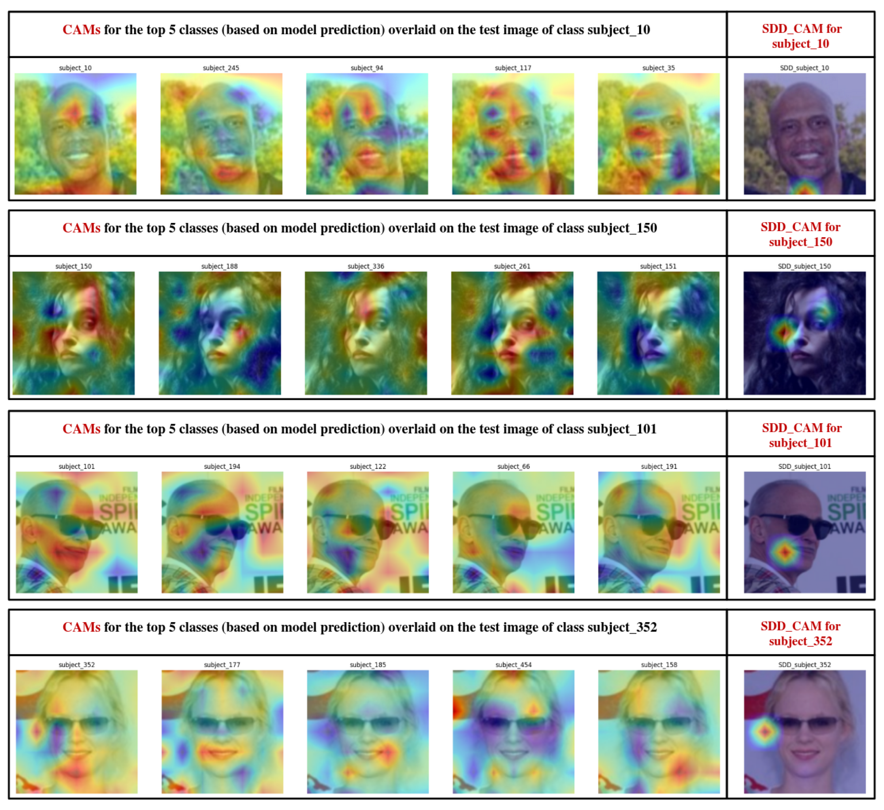
Here, we visually explain the prediction of the face recognition model. We describe the fine localization of the most relevant face features (considered significant by the model), which visually explains the prediction of the CNN model. We consider four test images of four different classes (subject_4, subject_120, subject_63, and subject_134) that belong to the test set.

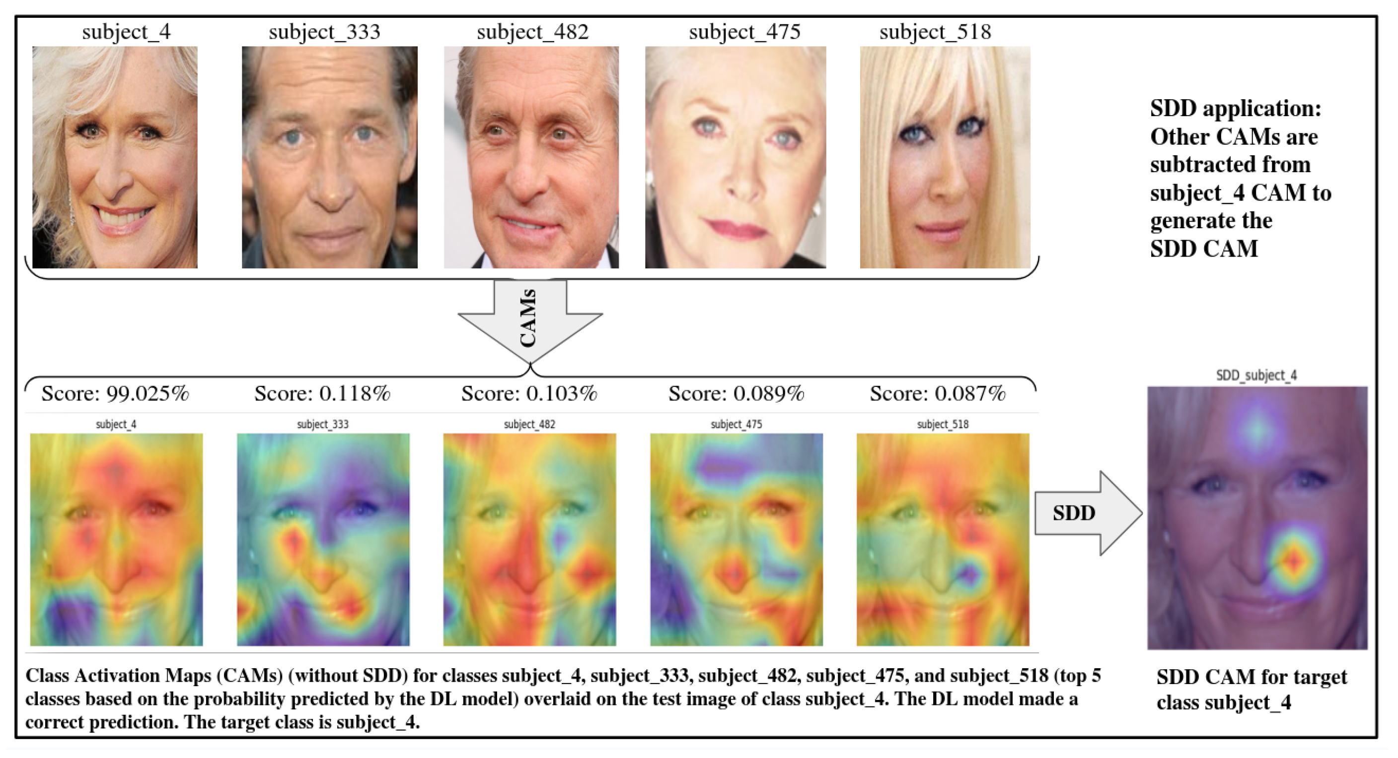
In Figure 3, the class of the test image is subject_4, which is predicted correctly by the face model. All the CAMs are overlaid on the test image of class subject_4. The target class is subject_4. For the SDD method, the top five classes (based on the probability predicted by the model) are considered. In the bottom row, the first five CAMs (from the left) are generated for the top five classes. The top row shows the sample images of the classes for which CAMs are generated. There is significant overlap among the CAMs of these classes. The last CAM (in the bottom row) is generated using SDD for target class subject_4, in which very narrow/specific localization (compared to the traditional CAM of class subject_4) of the most relevant face features is shown. The SDD CAM highlights the most important features of class subject_4 (with respect to the other four classes) for the correct prediction of the model.

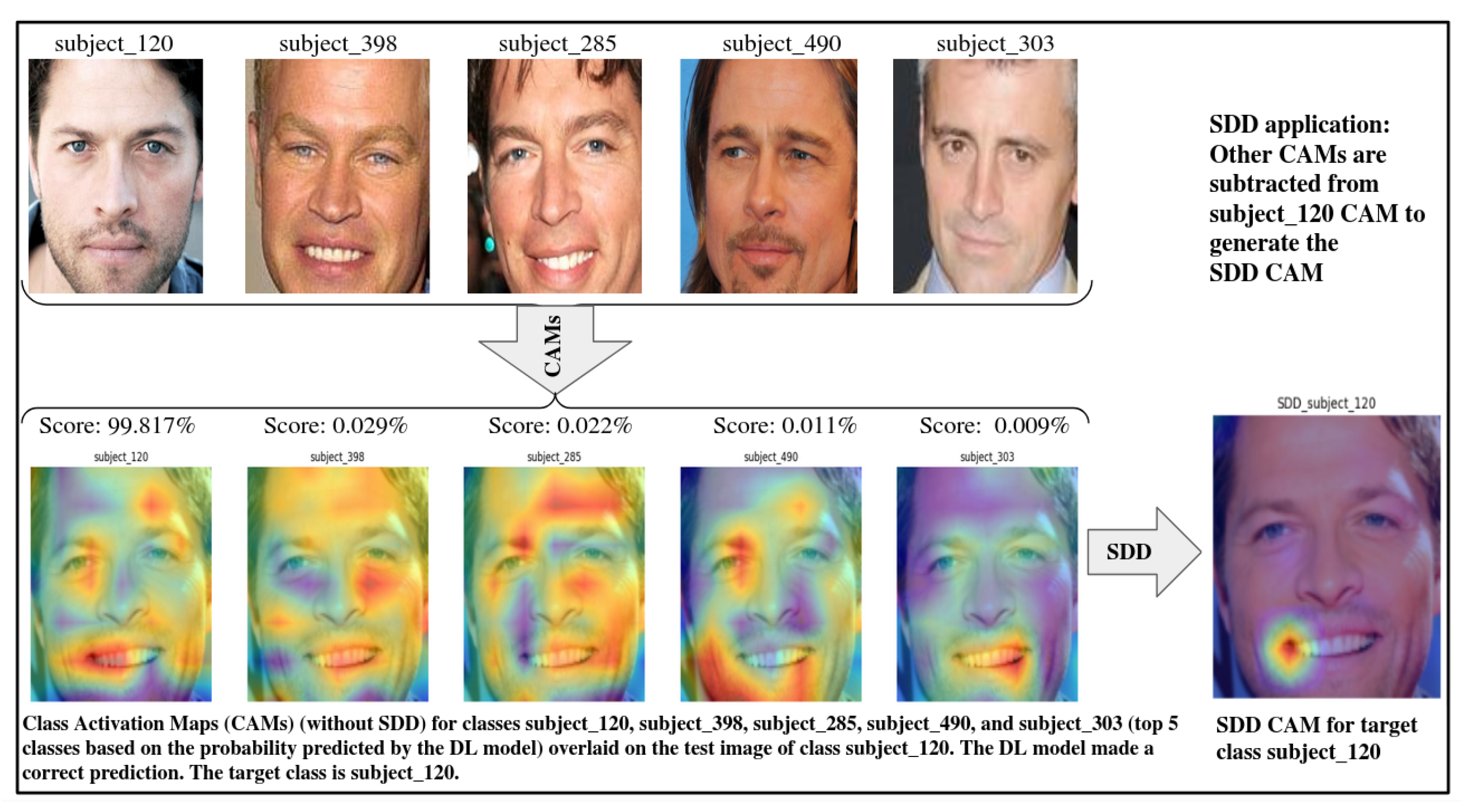
In Figure 4, the class of the test image is subject_120. The face model correctly predicted the class of the test image. Like the previous example, the CAMs are overlaid on the test image. The target class is subject_120. Same as before, the top five classes are considered for implementing the SDD method. The last CAM (in the bottom row) is generated using SDD for target class subject_120, in which very narrow/specific localization (compared to the traditional CAM of class subject_120) of the most relevant face features is shown. The SDD CAM highlights the most important features of class subject_120.

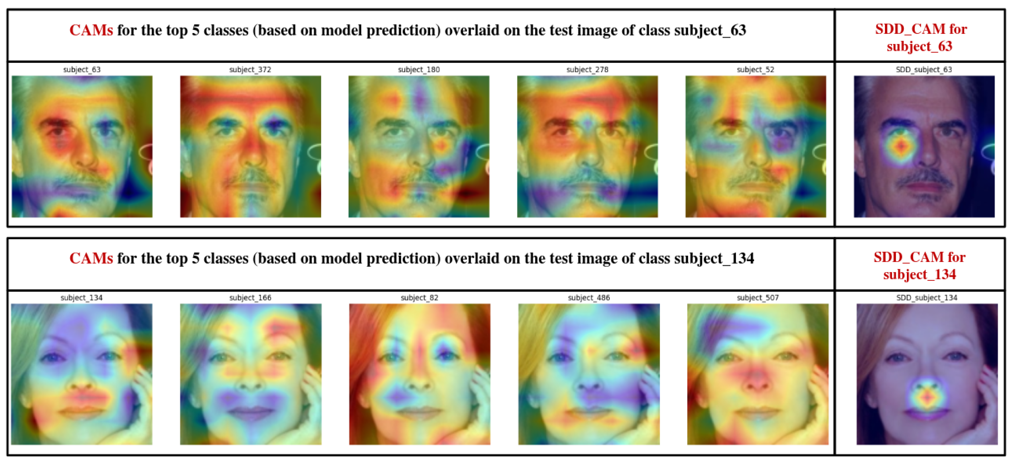
In Figure 5, two similar examples are shown. In the top row, the test image belongs to class subject_63 and is predicted correctly by the model. And in the bottom row, the test image belongs to class subject_134 and is predicted correctly by the model. In both cases, the top five classes (based on model prediction) are considered for the SDD method. The last column shows the SDD CAMs for classes subject_63 and subject_134, respectively.

4.2. Face Recognition Model—2

We use the same pre-trained AdaFace model, which is fine-tuned on a face dataset of 500 classes. This dataset is sampled from the CASIA-WebFace dataset [12] (a public dataset). The CASIA-WebFace is another high-quality and diverse dataset used for face recognition research. In the sampled dataset, there are a total of 500 classes (each person is a class). Among the 500 classes, there are both male and female classes. We divide the dataset into train, validation, and test sets with a ratio of 80/10/10. So there are 38,313 training images, 5046 validation images, and 4990 test images. The hyperparameters are the same as described in Section 4.1. The training time is around 1 h and 18 min. The overall test accuracy of the model is 81.86%.

Visual Explanation of Face Recognition

In this section, we show the same kind of examples for the face recognition model described above (as we showed earlier) in Figure 6. We have generated SDD CAMs for four test images. All the test images are predicted correctly by the model.

5. Evaluation of the Visual Explanation

In this section, we evaluate the visual explanations generated by the Scaled Directed Divergence method for the face recognition model. We use the deletion-and-retention evaluation scheme [19]. The deletion method evaluates the effectiveness of the visual explanations by removing the most important regions of an image identified by the explanation map and measuring the model’s confidence drop (a higher drop is better). In the case of the retention method, evaluation is performed by retaining the most significant regions of an image identified by the explanation map and measuring the model’s confidence drop (a lower drop is better).

5.1. Deletion

During deletion, we remove the top 20% values of the SDD CAM by replacing them with 0. We remove the top 20% values to demonstrate the impact of the most important regions highlighted in the SDD CAM. However, consider that the top 20% values removes more areas than highlighted in the SDD CAM. This is because the extra regions are also included in the top 20% values of the SDD CAM (though they are not highlighted).

Figure 7 shows an example of the deletion scheme. To compare with the important regions of the SDD CAM, we remove random areas of the same dimension (we call it random CAM). When certain regions of a test image are removed/covered, the prediction confidence of the face recognition model drops. When SDD CAM regions are removed/covered, the confidence drop should be higher. On the other hand, when random regions are removed/covered, the confidence drop should be lower.

For example, for a test image, the original confidence of the model is 99% (for the top class). When SDD CAM regions are removed, the confidence is 70% (for the original top class). So the confidence drop is 20%. When random regions are removed, the confidence should be higher than 70% and the confidence drop should be lower than 20%. This is because SDD CAM regions are more important for the prediction of the model than random regions. This hypothesis may not apply to all the test images, but it should be true for most of the test images. Therefore, we calculate the average confidence drop for the whole test set (4494 images) of the FaceScrub dataset as well as for the test set (4990 images) of the sampled CASIA-WebFace dataset, removing/covering the SDD CAM regions (making the top 20% values of the SDD CAM 0 as it demonstrates the impact properly). Also, we calculate the average confidence drop after removing/covering random regions of the same dimension.

Another metric to evaluate the SDD CAM results is the change in prediction. In many cases, the prediction of the model changes due to removing/covering certain areas of the test image. For deletion, the prediction change percentage for the whole test dataset should be higher in the case of SDD CAMs. In the case of random CAMs, the prediction change percentage should be lower. For the deletion method and the FaceScrub test set, the average confidence drop for SDD CAMs is 62.33%, whereas the average confidence drop for random CAMs is 42.50%. The prediction change percentage for SDD CAMs is 51.36%, whereas for random CAMs, the prediction change percentage is 29.73%. The results are shown in

Table 1. Performance comparison between SDD CAM and random CAM using the deletion method on the FaceScrub (4494 test images) and CASIA-WebFace (4990 test images) datasets.

Dataset	Metric	SDD CAM	Random CAM
FaceScrub	Average Confidence Drop	62.33%	42.50%
	Prediction Change Percentage	51.36%	29.73%
CASIA-WebFace	Average Confidence Drop	45.05%	26.83%
	Prediction Change Percentage	60.40%	37.90%

. For the CASIA-WebFace test set, the average confidence drop for SDD CAMs is 45.05%, whereas the average confidence drop for random CAMs is 26.83%. The prediction change percentage for SDD CAMs is 60.40%, whereas for random CAMs, the prediction change percentage is 37.90%. For both evaluation metrics—(1) Average Confidence Drop and (2) Prediction Change Percentage—and for both datasets, the explanations generated by SDD CAM outperform those of random CAM. This means that SDD CAM highlights more relevant image regions, leading to a greater drop in model confidence and more frequent prediction changes when those regions are removed/covered.

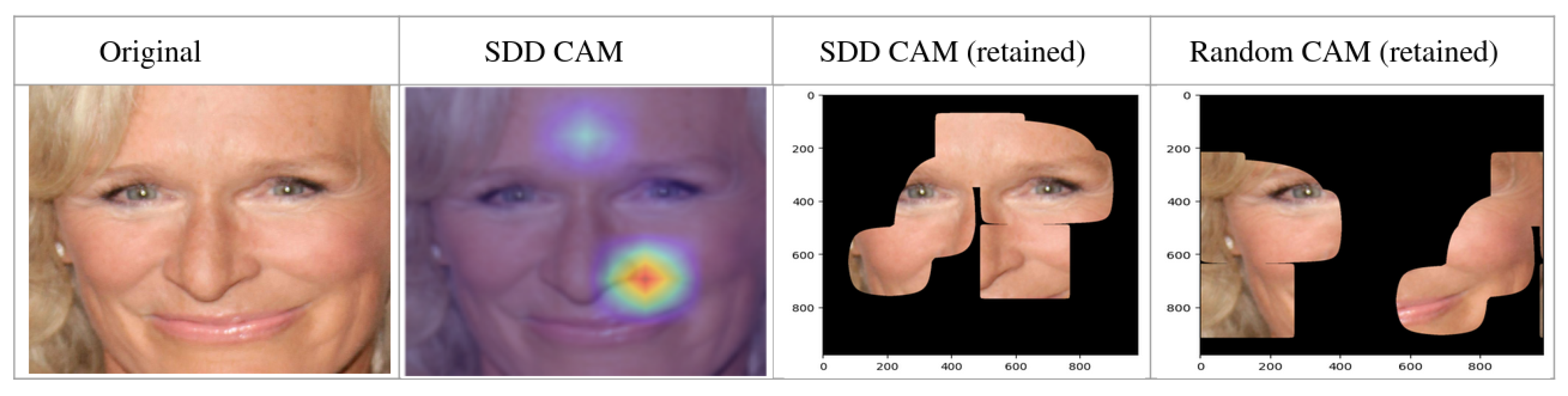
5.2. Retention

In the retention method, only those regions are retained that are removed/covered in the deletion method. Figure 8 shows an example of the retention scheme.

As only certain regions are retained, the prediction confidence of the model drops significantly in both the SDD CAM and random CAM cases. However, when the SDD CAM regions are retained, the confidence drop should be lower as the SDD CAM regions are the most relevant regions to the model. When random CAM regions are retained, the confidence drop should be higher, as these regions are not that significant in general. Also, the prediction change percentage should be lower for the SDD CAM than for the random CAM. In the case of the FaceScrub test set, the average confidence drop for the retention method is 69.43% for SDD CAMs. For random CAMs, the average confidence drop is 82.21% which is higher compared to the average drop for SDD CAMs. The prediction change percentage for SDD CAMs is 57.68% using the retention method. For random CAMs, the prediction change percentage is 79.93%, which is much higher. The results are shown in

Table 2. Performance comparison between SDD CAM and random CAM using the retention method on the FaceScrub (4494 test images) and CASIA-WebFace (4990 test images) datasets.

Dataset	Metric	SDD CAM	Random CAM
FaceScrub	Average Confidence Drop	69.43%	82.21%
	Prediction Change Percentage	57.68%	79.93%
CASIA-WebFace	Average Confidence Drop	46.30%	61.95%
	Prediction Change Percentage	59.98%	84.99%

. In the case of the CASIA-WebFace test set, the average confidence drop is 46.30% for SDD CAMs. For random CAMs, the average confidence drop is 61.95%. The prediction change percentage is 59.98% for SDD CAMs and 84.99% for random CAMs. The evaluation results clearly show that SDD CAM provides more effective explanations compared to random CAM.

5.3. Discussion

The SDD results show that the most relevant regions of a face that a deep learning model considers for making its prediction/decision can be localized very specifically (in a very narrow manner compared to the traditional CAM) using the SDD technique. The SDD explanations are evaluated using the deletion-and-retention scheme (Section 5). The evaluation results validate that the SDD CAM highlights the most important regions of a test image, which the face recognition model considers for its prediction. For the target class, the face features are determined with respect to other classes.

While the SDD technique is introduced effectively as a means to enhance class-discriminative localization, a comparison with traditional CAM in terms of computational efficiency and implementation complexity further supports its utility. Traditional CAM is computationally efficient and simple to implement, as it only requires a forward pass and access to the final convolutional feature maps and class weights. SDD builds on this framework by introducing additional steps, and specifically, by generating CAMs for non-target classes and computing the scaled divergence. Although this adds some computational overhead due to multiple forward passes or class-specific CAM generation, the implementation remains relatively straightforward within the same architectural pipeline. The additional cost is justified by the substantial improvement in localization precision and interpretability, particularly in class-overlapping or fine-grained scenarios. Thus, SDD strikes a practical balance between ease of integration and improved explanation quality, making it a compelling choice over a traditional CAM. With the GPU, it takes around 1.5 s to generate a SDD CAM from the CAMs of similar classes.

The face features highlighted in SDD CAMs are significant to the face recognition model for making its prediction. Such insight can be beneficial for explaining the behavior of deep learning-based face recognition models and increasing their transparency. Also, it will enhance trust in the decisions of the DL-based face recognition systems and can be used to improve their performance.

6. SDD Adaptability

SDD is method-agnostic and can serve as a refinement or alternative within the CAM family of techniques. It can be extended to work with other attribution maps by applying the SDD formulation over a set of such maps. In this section, we generate SDD Score-CAMs instead of SDD CAMs to demonstrate the SDD technique’s adaptability.

6.1. SDD Score-CAM

SDD Score-CAM is based on Score-CAM [13]. Score-CAM (Score-Weighted Class Activation Mapping) is a gradient-free visual explanation method proposed to improve the interpretability of CNNs. Unlike gradient-based techniques such as Grad-CAM, which rely on backpropagated gradients to assess the importance of activation maps, Score-CAM leverages the model’s prediction scores directly. Specifically, Score-CAM generates attention maps by first extracting activation maps from a chosen convolutional layer, then upsampling and normalizing them to create spatial masks. These masks are individually applied to the input image to form masked inputs, which are fed forward through the model to obtain class-specific confidence scores. The contribution of each activation map is quantified based on the score it yields, and the final class activation map is produced by a weighted combination of these maps using the corresponding scores as weights. This gradient-independent approach reduces noise and enhances the reliability of the visual explanations, making Score-CAM more robust and architecture-agnostic for interpreting CNN decisions.

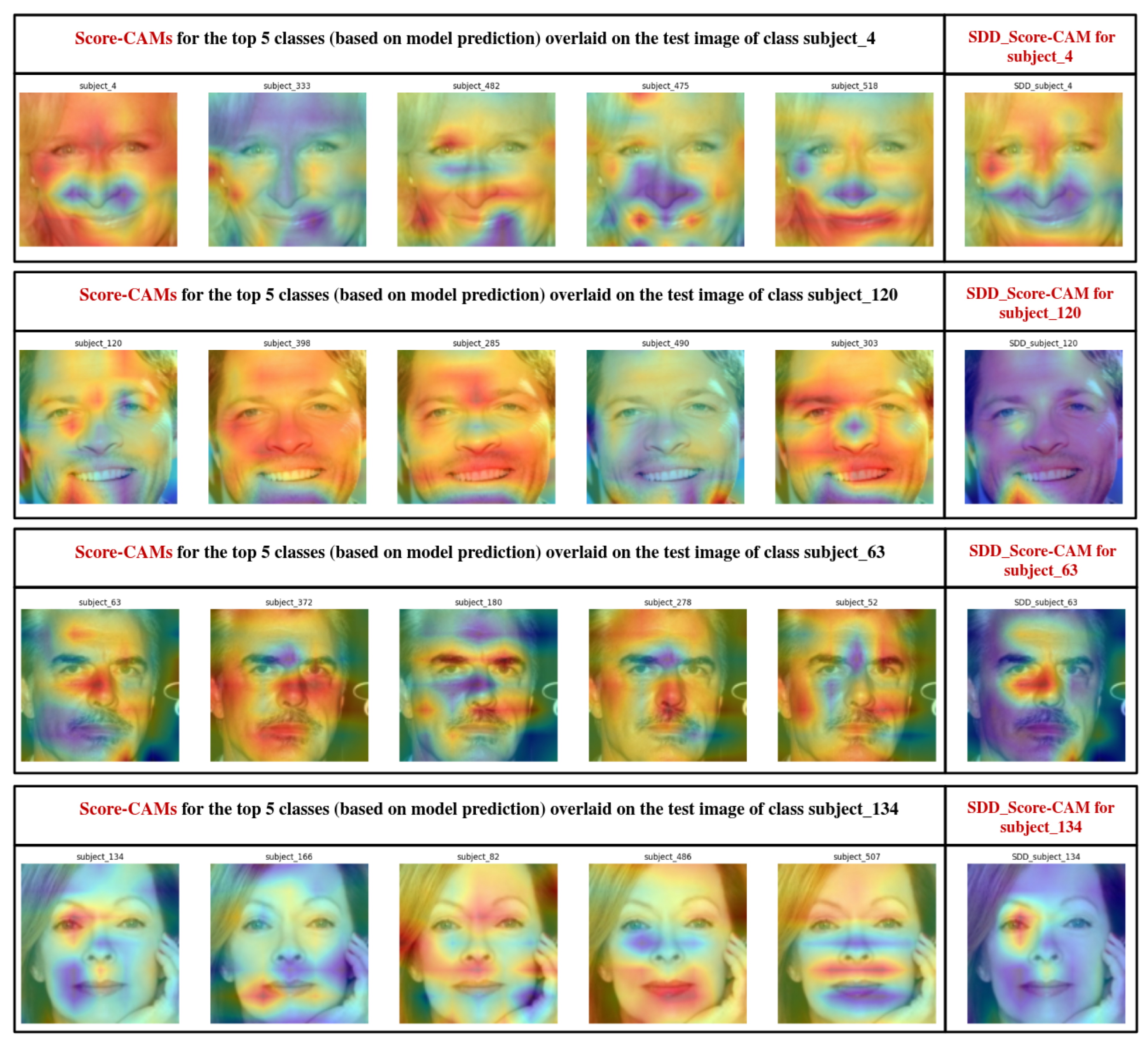
The details of the SDD framework described in Section 3.2 remain the same for generating SDD Score-CAM. Instead of a set of CAMs, a set of Score-CAMs is used to generate the SDD Score-CAM for the target class. Four examples are shown in Figure 9 for the test images of the FaceScrub dataset. In the first row, a test image of class subject_4 is considered for the SDD Score-CAM implementation. The model correctly predicted the class of the test image. Score-CAMs are generated for the top five classes (based on model prediction) and overlaid on the test image. The target class is subject_4. The last image in the row shows the SDD Score-CAM for class subject_4. Similarly, in the second row, a test image of class subject_120 is considered (correct prediction by the model). Score-CAMs are generated for the top five classes and overlaid on the test image. The last image in the row shows the SDD Score-CAM for the target class subject_120. Two more similar examples are shown in the third and fourth rows for a test image of class subject_63 (correct prediction by the model) and a test image of class subject_134 (correct prediction by the model), respectively. For the test images of the CASIA-WebFace dataset, SDD Score-CAMs are generated in Figure 10.

6.2. Evaluation of SDD Score-CAM Results

To evaluate the SDD Score-CAM results, we use the same deletion-and-retention method described in Section 5. We use the same two evaluation metrics: (1) Average Confidence Drop and (2) Prediction Change Percentage.

During deletion, we remove the top 20% values of the SDD Score-CAM, and we remove random areas of the same dimension (random CAM) to compare with the most important regions of the SDD Score-CAM. For the deletion method and the FaceScrub test set, the average confidence drop for SDD Score-CAMs is 39.17%, whereas the average confidence drop for random CAMs is 13.66%. The prediction change percentage for SDD Score-CAMs is 29.33%, whereas for random CAMs, the prediction change percentage is 7.85%. The results are shown in

Table 3. Performance comparison between SDD Score-CAM and random CAM using the deletion method on the FaceScrub (4494 test images) and CASIA-WebFace (4990 test images) datasets.

Dataset	Metric	SDD Score-CAM	Random CAM
FaceScrub	Average Confidence Drop	39.17%	13.66%
	Prediction Change Percentage	29.33%	7.85%
CASIA-WebFace	Average Confidence Drop	45.48%	11.44%
	Prediction Change Percentage	61.30%	20.84%

. For the CASIA-WebFace test set, the average confidence drop for SDD Score-CAMs is 45.48%, whereas the average confidence drop for random CAMs is 11.44%. The prediction change percentage for SDD Score-CAMs is 61.30%, whereas for random CAMs, the prediction change percentage is 20.84%. From the evaluation results, it is evident that SDD Score-CAM explanations are better than those of random CAM.

Only the top 20% of the SDD Score-CAM values are retained during the retention process. For the random CAM, these retained regions are shifted randomly. For the retention method and the FaceScrub test set, the average confidence drop for SDD Score-CAMs is 86.69%, which is lower than the average confidence drop for random CAMs (89.22%). The prediction change percentage for SDD Score-CAMs is lower (89.99%) than that for random CAMs (97.82%). In the case of CASIA-WebFace test set, the average confidence drop for SDD Score-CAMs is 54.39% (lower than the average confidence drop for random CAMs—66.79%). The prediction change percentage for SDD Score-CAMs is lower (70.60%) than that for random CAMs (96.33%). A lower average drop and prediction change are better for the retention method, which shows the effectiveness of SDD Score-CAM explanations. The results are shown in

Table 4. Performance comparison between SDD Score-CAM and random CAM using the retention method on the FaceScrub (4494 test images) and CASIA-WebFace (4990 test images) datasets.

Dataset	Metric	SDD Score-CAM	Random CAM
FaceScrub	Average Confidence Drop	86.69%	89.22%
	Prediction Change Percentage	89.99%	97.82%
CASIA-WebFace	Average Confidence Drop	54.39%	66.79%
	Prediction Change Percentage	70.60%	96.33%

.

6.3. Discussion

Despite traditional CAM being considered less precise than methods like Score-CAM, our results show that SDD-CAM, based on traditional CAM, outperforms SDD Score-CAM in deletion and retention evaluations. This is because traditional CAM inherently leverages class-specific weights from the final, fully connected layer, producing activation maps that are already focused on class-relevant features. When combined with SDD, these maps become even more discriminative by suppressing overlapping evidence from other classes. In contrast, Score-CAM, while generally strong for localization, generates broader activation maps that do not benefit as much from the SDD subtraction process. As a result, SDD CAM tends to highlight more compact and class-unique regions, which leads to a higher confidence drop and prediction change during deletion, and a lower drop and prediction change during retention, both of which indicate stronger explanation quality.

Another aspect is the computational efficiency. SDD Score-CAM combines the strengths of Score-CAM with the class-discriminative power of the SDD framework, but it comes with increased computational cost and implementation complexity. Unlike a traditional CAM, which requires only a single forward pass, Score-CAM involves multiple forward passes—one for each activation map masked input—to compute class-specific importance weights. Integrating SDD into this process further increases the load by requiring Score-CAM generation for non-target classes to perform the divergence-based subtraction. As a result, SDD Score-CAM is computationally more intensive, especially when applied to multi-class settings or high-resolution images. With the GPU, it takes around 27 s to generate a SDD Score-CAM from the Score-CAMs of similar classes. Despite these challenges, SDD Score-CAM can be beneficial in cases where broad localization is preferred.

7. Conclusions

This paper visually explains deep learning-based face recognition using an effective localization technique Scaled Directed Divergence. The experiments show that traditional CAMs perform broad localization of relevant face features and are unsuitable in the case of overlapping classes. The Scaled Directed Divergence technique based on CAM can perform very narrow/specific localization of the face features relevant to a deep learning-based face recognition model for making its prediction/decision. The visual explanations generated by the SDD technique are evaluated using the deletion-and-retention scheme. The evaluation results validate the effectiveness of the SDD technique in localizing the most significant face features. Also, the SDD technique is a flexible framework which can be used based on other CAM methods as well, such as Score-CAM. The evaluation results show that SDD Score-CAM may not be as effective as SDD CAM when very narrow/specific localization is preferred. Still, SDD Score-CAM provides narrower localization than Score-CAM. These visual explanations will increase the transparency and trustworthiness of existing and new deep learning-based face recognition models. The predictions/decisions of the face recognition models will be more acceptable to the end-users with proper explanations. Also, this can be used to improve the performance of the models by indicating the flaws and biases.