Research on Multi-Agent Collaborative Scheduling Planning Method for Time-Triggered Networks

Abstract

Time-triggered Ethernet combines time-triggered and event-triggered communication, and is suitable for fields with high real-time requirements. Aiming at the problem that the traditional scheduling algorithm is not effective in scheduling event-triggered messages, a message scheduling algorithm based on multi-agent reinforcement learning (MADDPG, Multi-Agent Deep Deterministic Policy Gradient) and a hybrid algorithm combining SMT (Satisfiability Modulo Theories) solver and MADDPG are proposed. This method aims to optimize the scheduling of event-triggered messages while maintaining the uniformity of time-triggered message scheduling, providing more time slots for event-triggered messages, and reducing their waiting time and end-to-end delay. Through the designed scheduling software, in the experiment, compared with the SMT-based algorithm and the traditional DQN (Deep Q-Network) algorithm, the new method shows better load balance and lower message jitter, and it is verified in the OPNET simulation environment that it can effectively reduce the delay of event-triggered messages.

1. Introduction

With the development of Industry 4.0, critical fields, such as aerospace, medical monitoring, and financial trading, have raised higher demands for communication networks, including high reliability, strong real-time performance, and determinism [1]. Systems in these industries often require data exchange under strict time constraints to ensure operational safety and efficiency. However, traditional Ethernet, due to its “best-effort” transmission mechanism [2], struggles to provide sufficient reliability and deterministic services when facing large-scale, high-density information exchanges. Consequently, Time-Triggered Ethernet (TTE), a novel network technology combining time-triggered mechanisms with the flexibility of traditional Ethernet, has emerged [3]. By utilizing predefined scheduling tables, TTE guarantees reliable and time-deterministic message transmission, demonstrating broad application prospects.

The design philosophy of TTE lies in retaining the characteristics of traditional Ethernet while incorporating redundancy, fault tolerance, and clock synchronization mechanisms from time-triggered technology [4], thereby achieving deterministic and real-time information interaction between network nodes. In TTE, message scheduling is a critical factor in ensuring network performance [5]. Traditional scheduling algorithms, though capable of generating feasible solutions, exhibit limitations in optimizing event-triggered message scheduling, leading to significant delays and potential jitter for such messages.

To address TTE message scheduling challenges, researchers have proposed various algorithms. For example, Steiner et al. introduced a static scheduling table generation method based on Satisfiability Modulo Theories (SMT) [6], while Pozo et al. proposed a segmented solving strategy [7]. Trüb et al. adopted a linear programming (LP) approach to unify task and network resource scheduling [8]. Additionally, scheduling algorithms based on mixed-integer nonlinear programming (MINLP) [9] and genetic algorithms have been explored. Although these algorithms partially resolve scheduling issues, their effectiveness in optimizing event-triggered messages remains limited, particularly under increased network loads, where delays and jitter may escalate.

Multi-Agent Reinforcement Learning (MARL) has recently gained attention for its advantages in handling resource allocation problems in complex environments [10]. In TTE message scheduling, MARL enables agents to learn superior strategies that adapt to dynamic network conditions. For instance, Miyazaki et al. utilized the Multi-Agent Deep Deterministic Policy Gradient (MADDPG) to support collaborative transportation among industrial robots [11]; Lei et al. applied MADDPG to optimize smart grid resource allocation [12]; Jiang et al. extended it to multi-object tracking in computer vision [13]; Novati et al. explored its potential in automated turbulence model discovery [14]; Li et al. employed MARL for crowd simulation and multi-character control [15]. In domestic research, Zhao Cong et al. improved regional parking space allocation through MARL [16]; Yang et al. enhanced MADDPG for UAV swarm confrontation; Dong Lei et al. proposed a MARL-based solution for electro-thermal integrated energy system optimization [17] and Ye Lin et al. leveraged reinforcement learning agents to adjust grid-controllable resources for power system security.

1.1. Limitations of Existing Methods

SMT-Based Static Scheduling:

While Satisfiability Modulo Theories (SMT) solvers [7] can generate feasible schedules by strictly adhering to TTE constraints, they lack optimization capabilities. This results in densely packed TT message allocations, leaving minimal idle slots for RC/BE messages. Consequently, event-triggered messages experience high end-to-end delays and jitter under dynamic network loads [6].

Single-Agent Reinforcement Learning (DQN):

Deep Q-Network (DQN)-based approaches [12] attempt to optimize scheduling through trial-and-error learning. However, their single-agent architecture struggles to coordinate distributed TT messages in large-scale networks. For instance, in scenarios with 190 TT messages (Experiment 4), DQN’s training efficiency degrades by 0.37 compared to small-scale cases, leading to suboptimal load balancing and prolonged convergence times.

1.2. Proposed Approach

To overcome these limitations, we propose a Multi-Agent Deep Deterministic Policy Gradient (MADDPG)-based scheduling framework with two novel contributions:

Collaborative Multi-Agent Optimization:

Each TT message operates as an independent agent that dynamically negotiates scheduling offsets. By leveraging centralized critics to share global link load information (Section 3.2).

Hybrid SMT-MADDPG Initialization:

The initialization accelerates convergence while maintaining a 0.43 improvement in load balancing over pure SMT.

1.3. Key Advantages

Adaptive Scheduling: MADDPG agents dynamically adjust to network topology changes, outperforming static SMT schedules in scenarios with varying traffic loads (Section 4.3).

Scalability: Multi-agent coordination enables efficient scheduling in large-scale networks (Experiment 2), where DQN fails to converge.

2. Time-Triggered Network Scheduling Planning Model

In order to make TTE message scheduling more clear, this paper transforms the scheduling problem in time-triggered Ethernet into a mathematical form, and symbolically describes the topology information, message information, network configuration information, scheduling rules and scheduling schedule in time-triggered Ethernet.

2.1. Time Triggered Network Model

In TTE, message types include Time-Triggered (TT), Rate-Constrained (RC), and Best-Effort (BE) messages. As shown in Figure 1, during the scheduling planning of TTE network, all devices in the network topology and messages in the network participate in the scheduling.

For all kinds of information in time-triggered Ethernet, the following definitions are made:

• All nodes in the network are defined as $ND$, the end system is defined as $ES$, and the switch used for forwarding is defined as $SW$, $SW\in ND$ and $ES\in ND$;
• In time-triggered networks, all physical link sets are defined as P that any physical link p in the network belongs to a set P, that is $p\in P$, both ends of any physical link $p_i$ in the network are network nodes $(n{d}_j,n{d}_k)$, respectively, and the link $p_i$ uniquely corresponds to the combination of network nodes $(n{d}_j,n{d}_k)$;
• Because the network transmission of physical links uses the same medium, the network bandwidth is defined as $NET.bw$; $NET$ represents the network;
• A complete set of message transmission paths is a virtual link, which $VL$ represents the set of all virtual links. For any one $vl\in VL$, it can be represented by an ordered set of physical links p, that is $vl=\{p_1,p_2,p_3,p_4,\cdots ,p_n\}$, it represents a complete message transmission path;
• The set of all messages in the network is represented by $MF$, including all messages in the network.

2.2. Time-Triggered Network Scheduling Constraints

The constraint condition of a time-triggered network is the prerequisite to ensure the successful scheduling of messages. According to the time-triggered network communication scheduling, the schedule must satisfy the following constraints:

2.2.1. Basic Periodic Constraint

In the final generated scheduling result, for all messages with periodic characteristics, the final scheduling time should be after 0 and 0 and before the corresponding cycle end time.

2.2.2. One-Cycle Completion Constraint

The sending of TT messages in the network follows the periodic law, that is, the scheduling of each message should be completed in its own period. Assuming that the period of a message is 1ms, the whole process of transmission is completed at least once in one period of the message. However, in the actual situation, because of network delay, message jitter and other reasons, the message is not scheduled in the current cycle, and the time slot reserved in advance is also needed to ensure that the message scheduling can be performed normally when the time slot of the next cycle comes. In this model, the influence of propagation delay is ignored, and only transmission delay is considered.

2.2.3. Scheduling Time Sequence Constraint

This constraint requires the scheduling order of messages from the source system to the destination system, that is, the time sequence that any message needs to follow in the process of scheduling on a transmission path. This constraint is aimed at the message itself.

2.2.4. End to End Delay Constraint

When scheduling and planning, messages are sent from the source system to the destination system and pass through one or more switch devices in the middle. There should be a maximum tolerable delay in the whole transmission process, that is, the maximum time consumption should be limited to a certain range. In most cases, the end-to-end delay of a message is the period of the message.

Minimize End-to-End Delays of Event-Triggered Messages:

Reduce the average delay for Rate-Constrained (RC) and Best-Effort (BE) messages.

$$\mathrm{Objective}1:min\left({\displaystyle \frac{1}{N_{RC}}}{\sum }_{i=1}^{N_{RC}}E{D}_i^{RC}+{\displaystyle \frac{1}{N_{BE}}}{\sum }_{j=1}^{N_{BE}}E{D}_j^{BE}\right)$$

where $E{D}_i^{RC}$ and $E{D}_j^{BE}$ represent the end-to-end delay of the i-th RC and j-th BE message, respectively.

The message is sent from the source network node to the destination network node (as shown in Figure 2, the path es1-sw1-sw2-es4) after being transited by two switch devices. The total transmission delay calculation method is:

$$\begin{array}{cc}\hfill \forall m{f}_i\in MF,m{f}_i·delay\_all& =m{f}_i^{e{s}_1}·delay+m{f}_i^{s{w}_1}·delay+m{f}_i^{s{w}_2}·delay\hfill \\ & ={\displaystyle \frac{m{f}_i·length}{NET.bw}}+{\displaystyle \frac{m{f}_i·length}{NET.bw}}+{\displaystyle \frac{m{f}_i·length}{NET.bw}}\hfill \\ & =3\ast {\displaystyle \frac{m{f}_i·length}{NET.bw}}\hfill \end{array}$$

(1)

From the above, it can be seen that the time consumption of message transmission is related to the number of network nodes through which the message will pass, and the total transmission delay of the message is the sum of the transmission delays on each network node. The formula is expressed as follows:

$$\begin{array}{cc}\hfill \forall m{f}_i\in MF,m{f}_i·delay\_all& =m{f}_i^{e{s}_1}·delay+m{f}_i^{e{s}_2}·delay+\cdots +m{f}_i^{e{s}_k}·delay\hfill \\ & ={\displaystyle \frac{m{f}_{i}length}{NET.bw}}+{\displaystyle \frac{m{f}_{i}length}{NET.bw}}+\cdots +{\displaystyle \frac{m{f}_{i}length}{NET.bw}}\hfill \\ & =k\ast {\displaystyle \frac{m{f}_{i}length}{NET.bw}},k\in N+\hfill \end{array}$$

(2)

Therefore, the end-to-end delay of a message is closely related to the length of the message, the link bandwidth in the network, the number of network nodes it will experience, and the forwarding delay of the message in the switch.

2.3. Unique Challenges in TTE Scheduling

Novelty of MARL/MADDPG in TTE Scheduling: Unique Challenges and Innovations The application of Multi-Agent Reinforcement Learning (MARL) and Multi-Agent Deep Deterministic Policy Gradient (MADDPG) to Time-Triggered Ethernet (TTE) scheduling introduces distinct innovations tailored to address challenges absent in traditional applications like smart grids or robotic control. Below, we clarify the unique aspects of TTE scheduling and explain how the proposed MARL framework overcomes them.

1. Strict Real-Time Determinism

Challenge: TTE networks require deterministic message transmission with bounded end-to-end delays (e.g., sub-microsecond precision in aerospace systems).

Difference from Other Domains:

Smart Grids: Prioritize stability over strict timing.

Robot Control: Focus on collision avoidance and path planning, not nanosecond-level synchronization.

2. Hybrid Traffic Coexistence

Challenge: TTE integrates time-triggered (TT), rate-constrained (RC), and best-effort (BE) traffic, requiring simultaneous optimization of conflicting priorities.

Difference:

Smart Grids: Primarily handle continuous energy flow without sharp priority divisions.

Robot Swarms: Focus on homogeneous task allocation, not mixed-criticality scheduling.

3. Dynamic Network Scalability

Challenge: TTE networks must adapt to dynamic node additions/removals (e.g., plug-and-play avionics modules) while maintaining schedulability.

Difference:

Smart Grids: Infrastructure changes are rare and planned.

Robot Teams: Fixed team size during missions.

4. Complex Constraint Interdependencies

Challenge: TT messages have path-dependent constraints (e.g., sequential transmission across switches) and global hypercycle alignment.

Difference:

Smart Grids: Constraints are localized (e.g., voltage limits).

Robot Coordination: Constraints focus on spatial relationships, not temporal dependencies.

3. Message Scheduling Based on Multi-Agent Reinforcement Learning

We adopt the principle of centralized training and distributed execution, introduce centralized critic networks utilize global network information to guide the training of decentralized policy networks, and design the state space, action space, scheduling index and return function of the algorithm, and introduce the implementation process of the algorithm in detail, so that multiple agents can accumulate experience through continuous exploration and use the evaluation index to continuously update the algorithm model, so that the algorithm can obtain a better scheduling solution in the process of continuous training. In this paper, the scheduling problem in time-triggered Ethernet is combined with multi-agent reinforcement learning, and two message scheduling algorithms for time-triggered networks are proposed:

• Time-triggered network message scheduling and planning algorithm based on the MADDPG algorithm. The principle of centralized training and decentralized execution is adopted, and global information is introduced to guide algorithm training;
• A hybrid scheduling algorithm of MADDPG based on SMT experience initialization. The feasible solution obtained by the SMT mathematical algorithm is transformed into an initial experience to guide the algorithm in training, thus reducing the initial training burden of the MADDPG algorithm.

3.1. Message Scheduling Planning Model Based on Multi-Agent Reinforcement Learning

The scheduling model set in this paper is composed of Markov decision sextuples $<G,S,A,\pi ,H,R>$.

• Agent Set G: Each time-triggered (TT) message $m_i\in {\mathcal{MF}}_{TT}$ is modeled as an agent $g_i\in G$. Each agent is responsible for making scheduling decisions for its own message across all required links along its virtual path.
• State S: The global state S represents the current scheduling occupation of all physical links in the network. Formally,

  $$S=\{{\mathrm{Slot}}_{p,t}\mid p\in \mathcal{P},t\in [0,H)\}$$

  where ${\mathrm{Slot}}_{p,t}\in \{0,1\}$ indicates whether the time slot t on the physical link p is occupied (1) or free (0), and H is the scheduling hyperperiod. This provides the agent with visibility into available transmission slots along the path.
• Action A: The action $a_i$ of the agent $g_i$ is to select a feasible offset time $o_i$ from a discretized candidate set:

  $$A_i=\{o_i\in [0,H)\mid \mathrm{offset}\mathrm{of}\mathrm{first}\mathrm{transmission}\mathrm{frame}\mathrm{of}{m}_i\}$$
  $A_i$ determines the starting time of message $m_i$’s periodic transmission. The agent’s action implicitly determines frame placements across all links in the message’s virtual link path.
• Policy $\pi$: Each agent has a stochastic policy ${\pi }_i(o_i\mid s_i)$, mapping observed local state $s_i$ (e.g., link availability along the path) to a probability distribution over actions (offsets). The joint policy is $\pi =\{{\pi }_1,\cdots ,{\pi }_N\}$.
• Interaction H (Policy iteration function): The learning framework follows the MADDPG setup with centralized training and decentralized execution. A global critic $Q_i(S,A)$ observes all agent actions and the global state to compute gradients for each actor policy ${\pi }_i$. During execution, each agent uses only its local state $s_i$ for decision making.

3.2. Scheduling Planning Method Based on MADDPG Algorithm

3.2.1. Elements of the MADDPG Scheduling Algorithm for Time-Triggered Network Scheduling Planning

1. State design of dispatching planning

When planning and scheduling messages, the performance of successful scheduling is that the scheduling results of all messages meet the scheduling constraints of the network. The message status of successful one-time scheduling is shown in Figure 3 below, which shows the message frame scheduling of three TT messages TT0, TT1 and TT2 on the link sent from network node A to network node B. In Figure 4, the message frames scheduled by TT0 and TT1 collide, and the message frames scheduled by TT2 and TT3 also collide, indicating that the scheduling is a failed scheduling.

2. Action design of dispatching planning

Message planning in time-triggered networks divides all the scheduling actions of messages into multiple message frames on different links. In the system, each message agent performs actions based on the corresponding policies. Because messages will transit through one or more switches during transmission, message agents will perform actions to select scheduling time for many times, and all the actions performed by each message agent must meet the constraint requirements.

3. Design of Return Function for Dispatching Planning

The priority of messages in the scheduling plan is TT>RC>BE. However, for the final scheduling result, the reward function should not only satisfy the success of TT message scheduling, but also consider the load balance of the scheduling result. When planning, we should try our best to prevent the message scheduling from being very closely arranged. On the premise of meeting the scheduling constraints of TT messages, we must also leave enough time slices for other messages to ensure that event-triggered messages can be sent as soon as possible when they need to be sent, so as to prevent large delay or jitter caused by too long waiting time.

Maximize Load Balancing Across Network Paths:

Ensure uniform distribution of idle gaps between TT messages to accommodate RC/BE traffic.

$$\mathrm{Objective}2:min\left(PL{B}_{ALL}\right)=min\left({\displaystyle \frac{1}{M}}{\sum }_{k=1}^{M}PL{B}_k\right)$$

where $PL{B}_k=\sqrt{{\displaystyle \frac{1}{n^{p_k}}}{\sum }_{j=1}^{n^{p_k}}{\left(ga{p}_j^{p_k}-{\overline{GAP}}^{p_k}\right)}^2}$, representing the load imbalance of the k-th path.

As shown in Figure 5 below, this figure shows the message scheduling situation on a certain path in the network. In this scheduling situation, TT messages are distributed in a scattered way, which is beneficial for better scheduling event-triggered messages and preventing event-triggered messages from causing large delays or jitters due to too long a waiting time.

The scheduling load balance index of TT messages on a certain path $p_i$ in the network can be expressed:

$$PL{B}_{p_i}=\sqrt{\sum _{i=1}^n{\left(ga{p}_j^{p_i}-{\overline{GAP}}^{p_i}\right)}^2/n^{p_i}}$$

(3)

where $PL{B}_{p_i}$ represents the load balance of path $p_i$, $ga{p}_j^{p_i}$ represents the length of j-th idle gap in path $p_i$, ${\overline{GAP}}^{p_i}$ represents the average length of the idle gap in the path $p_i$, and $n^{p_i}$ represents the number of idle gaps on the path $p_i$.

In the network, the scheduling time gap of message frames on a path determines the load situation on the path, as shown in Figure 6, which is the load balance of TT message scheduling in a super cycle on a certain path.

The load balance of global network scheduling can be expressed by the average value of scheduling load balance indicators of TT messages of each path $p_i$:

$$PLB\_ALL=\sum _{i=1}^m\left(PL{B}_i\right)/m$$

(4)

where $PLB\_ALL$ represents the load balance of all paths in the network, m represents the number of paths in the network, and $PL{B}_i$ represents the load balance of the i-th path.

Based on the above two evaluation index formulas, the load balance of all paths in the network can be used as the evaluation index of message scheduling under the premise of ensuring the success of scheduling.

There is no priority order among TT messages, but with the progress of message scheduling, it is more difficult to choose a strategy for messages with post-scheduling, because the selection range of messages with post-scheduling is too small due to improper strategy of previous messages, so in the training process, with the progress of message scheduling, the punishment for scheduling failure should be gradually reduced.

$$\begin{array}{cc}& R=\left\{\begin{array}{cc}\lambda {\displaystyle \frac{\mathrm{C}}{PLB\_ALL}},\hfill & \mathrm{All}\mathrm{message}\mathrm{scheduling}\mathrm{ends}\hfill \\ & \\ \eta {\displaystyle \frac{i}{M}},\hfill & \mathrm{The}\mathrm{i}-\mathrm{th}\mathrm{message}\mathrm{was}\mathrm{dispatched}\mathrm{successfully}.\hfill \\ & \\ -1+\eta {\displaystyle \frac{i}{M}},\hfill & \mathrm{The}\mathrm{i}-\mathrm{th}\mathrm{message}\mathrm{scheduling}\mathrm{failed}.\hfill \\ \end{array}\right.\hfill \\ & s.t.\left\{\begin{array}{cc}\lambda \in (0,1]\hfill & \\ \mathbb{C}\in {\mathbb{N}}^{\ast }\hfill & \\ \eta \in (0,1]\hfill & \\ i\in [1,M]\hfill \end{array}\right.\hfill \end{array}$$

(5)

The meaning and motivation of each component are described as follows:

• $\lambda$ ($\in (0,1]$): Controls the weight of the global reward term. It reflects the importance of achieving a well-balanced overall schedule once all messages are placed. A lower $\lambda$ reduces sensitivity to global balance, while a higher $\lambda$ emphasizes system-wide optimization.
• C ($\in {\mathbb{N}}^{+}$): A scaling factor that amplifies the global reward value and prevents vanishing gradients when ${\mathrm{PLB}}_{\mathrm{ALL}}$ is large. It does not affect convergence direction, but it affects learning speed.
• $\eta$ ($\in (0,1]$): The local scheduling reward coefficient. It provides intermediate feedback for successful message placements during partial scheduling, encouraging agents to make progress even before global completion.
• ${\displaystyle \frac{i}{M}}$: The normalized scheduling order of message i, where M is the total number of messages. This value increases over time, meaning earlier agents receive higher penalties if they fail. This design encourages earlier agents to act cautiously and leave more scheduling flexibility for later agents.
• ($-1+\eta ·{\displaystyle \frac{i}{M}}$): This gradually increasing penalty discourages poor decisions by early agents, which have a larger influence on downstream feasibility. Later agents receive milder penalties for failure, acknowledging their more constrained decision space.

Hyperparameter Selection

The hyperparameters $\lambda$, $\eta$, and C are selected through empirical tuning based on scheduling success rate, convergence stability, and message delay metrics in simulated environments. The following values were found effective:

In summary, the reward function design encourages agents to schedule their messages both successfully and cooperatively, while optimizing the overall time slot distribution to reduce delay and jitter for non-TT traffic.

3.2.2. Scheduling Algorithm Flow Based on MADDPG

1. Algorithm description

The MADDPG algorithm adopts the principle of centralized training and distributed execution, so it is suitable for a complex multi-agent environment. The MADDPG algorithm allows the Critic, who can observe all the information, to guide the training for each Actor. The critic can observe all the information in the whole world and guide the corresponding actors to optimize their strategies, but the actors who can only observe local information take action when the application is executed.

There is a message agent in the MADDPG algorithm. The policy of the message agent is expressed as ${\pi }_i$, the policy parameter is expressed as ${\theta }_i$, the policy set of the message agent is expressed as $\pi ={\pi }_1,{\pi }_2,{\pi }_3,\cdots ,{\pi }_N$, and the policy parameter set is expressed as $\pi ={\theta }_1,{\theta }_2,{\theta }_3,\cdots ,{\theta }_N$. All expected returns of message agents are expressed as follows:

$$J\left({\theta }_i\right)=\mathbb{E}\left[R_i\right]={\mathbb{E}}_{s-{\rho }^{\pi },{\alpha }_i-{\pi }_{{\theta }_i}}\left[\sum _{t=0}^{\infty }{\gamma }^t{r}_{i,t}\right]$$

(6)

where $\mathbb{E}\left[R_i\right]$ represents all expected returns of the ith message agent, and $r_{i,t}$ represents the return value of the message agent i at time t.

The policy gradient of each message agent for a random policy can be expressed as follows:

$${\nabla }_{{\theta }_i}=\mathbb{E}\left[{\nabla }_{{\theta }_i}ln\left(a_i\mid o_i\right)·Q_i^{\mu }\left(s,a_1,\cdots a_N\right)\right]$$

(7)

where $a_i$ represents the action of the message agent based on a random strategy, $o_i$ represents the observation value of the message agent, $Q_i^{\mu }\left(s,a_1,\cdots a_N\right)$ represents the value function of the agent based on a deterministic strategy, and S refers to the observation vector, that is, the state.

In the formula, $Q_i^{\mu }\left(s,a_1,\cdots a_N\right)$ is a global function, including its own state and the action $\left[a_1,a_2,a_3\cdots ,a_N\right]$ of all message agents. The policy network of message agents not only knows the changes of their own agents, but also knows the actions of other message agents.

The action value $a_i$ of the message agent i in the network based on a deterministic policy is as follows:

$$a_i={\mu }_i\left(o_i\right)+N_t$$

(8)

where ${\mu }_i\left(o_i\right)$ represents the deterministic strategy output by the strategy network of the agent i when observing the value $o_i$, and $N_t$ represents the action of the agent i based on the deterministic strategy ${\mu }_i$.

The formula for updating the expected return strategy network is as follows:

$${\nabla }_{{\theta }_i}J\left({\mu }_i\right)={\mathbb{E}}_{s,\mathrm{a}\sim \mathrm{D}}\left[{\nabla }_{{\theta }_i}{\mu }_i\left(a_i\mid o_i\right){\nabla }_{a_i}{Q}_i^{\mu }\left(s,a_1,\cdots a_N\right){|}_{a_i={\mu }_i\left(o_i\right)}\right]$$

(9)

where D represents the experience pool for storing all message agents, ${\mu }_i$ represents the deterministic strategy of the agent i, $a_i$ represents the actions of the agent i based on the deterministic strategy ${\mu }_i$, and $Q_i^{\mu }\left(s,a_1,\cdots a_N\right)$ represents the value function of the agent i based on the deterministic strategy ${\mu }_i$.

$Q_i^{\mu }$ establishes a value function for each agent, and its updating method draws lessons from TD-error mode and target network thought in DQN. The updated formula for evaluating the network is as follows:

$$L\left({\theta }_i\right)={\mathbb{E}}_{s,a,r,s^{\prime }}\left[{\left(Q_i^{\mu }\left(s,a_1,\cdots ,a_N\right)-y\right)}^2\right],y=r_i+\gamma Q_i^{{\mu }^{\prime }}(s^{\prime },a_1^{\prime },\cdots ,a_n^{\prime }){|}_{a_j^{\prime }={\mu }_j^{\prime }\left(o_j\right)}$$

(10)

where $L\left({\theta }_i\right)$ represents the loss function of the evaluation network, y represents the action value function, ${\mu }^{\prime }$ is $\left[{\mu }_1^{\prime },{\mu }_2^{\prime },{\mu }_3^{\prime },...,{\mu }_N^{\prime }\right]$, and $\gamma$ represents the discount factor, $\gamma \in [0,1]$.

In the above formula, the algorithm can estimate the strategies of other message agents. ${\widehat{\mu }}_{{\varphi }_i^j}$ represents the functional approximation of the i-th message agent to the j-th message agent strategy ${\mu }_j$. The loss cost function is expressed as follows:

$$L\left({\varphi }_i^j\right)=-{\mathbb{E}}_{o_j,a_j}\left[ln{\widehat{\mu }}_{{\varphi }_i^j}\left(a_j\mid o_j\right)+\lambda H({\widehat{\mu }}_{{\varphi }_i^j})\right]$$

(11)

where ${\widehat{\mu }}_{{\varphi }_i^j}$ represents the functional approximation of the i-th agent to the j-th agent strategy ${\mu }_j$, and $H({\widehat{\mu }}_{{\varphi }_i^j})$ represents the entropy of the strategy.

By reducing the cost function, the approximation $\widehat{y}$ of other agent strategies is obtained, and its calculation formula is expressed as follows:

$$\widehat{y}=r_i+\gamma {\overline{Q}}_i^{{\mu }^{\prime }}(s^{\prime },{\widehat{a}}_i^{\prime 1},{\widehat{a}}_i^{\prime 2},{\widehat{a}}_i^{\prime 3},\cdots ,{\widehat{a}}_i^{\prime N}){|}_{{\widehat{a}}_i^{\prime }={\widehat{\mu }}_i^{\prime }\left(o_i\right)}$$

(12)

The goal of training is to improve the return $J\left({\mu }_i\right)$ of the strategic network and reduce the loss $L\left({\theta }_i\right)$ of the evaluation network. The updated formulas are as follows:

$${\theta }_i\leftarrow {\theta }_i+\alpha {\nabla }_{{\theta }_i}J\left({\mu }_i\right),{\theta }_i\leftarrow {\theta }_i-\alpha {\nabla }_{{\theta }_i}L\left({\theta }_i\right).$$

(13)

where $\alpha$ represents the learning rate of the strategic network, that is, the update rate of the strategic network and the evaluation network in the network.

The update formula of the target network is as follows:

$${\theta }_i^{\prime }\leftarrow \tau {\theta }_i+(1-\tau ){\theta }_i^{\prime }$$

(14)

where $\tau$ represents the target network update rate $\tau \in [0,1)$.

When updating the network, the data of the same moment are randomly obtained from the experience pool of the message agent, and the new experience $<S,A,S^{\prime },R>$ is obtained by splicing them. Input S’ into the target strategy network of the ith message agent to obtain action A’, then input A’ and S’ into the target evaluation network of the ith message agent together to obtain the target Q value estimated at the next moment, and calculate the target Q value at the current moment according to the formula.

$$y_i=r_i+\gamma Q^{\prime }(s_{i+1},{\mu }^{\prime }(s_{i+1}\mid Q^{{\mu }^{\prime }})|{\theta }^{Q^{\prime }})$$

(15)

In the execution stage, the message agent relies on the optimized policy network to guide the agent’s strategy, inputs the local observation $o_i$, and outputs the scheduling action through the operation of the policy network. After each action selection, it is necessary to judge whether the action meets the constraint conditions. If not, it will give a negative return value and return to re-schedule. When all messages are successfully scheduled, the result scheduling schedule is obtained.

3.3. MADDPG Hybrid Scheduling Algorithm Based on SMT Empirical Initialization

3.3.1. Theoretical Basis of SMT Technology

The Satisfiability Modulo Theories (SMT) solver generates feasible schedules by resolving constraints in first-order logic. While SMT alone cannot optimize load balancing, its deterministic solutions provide reliable initial schedules for MADDPG training. By converting SMT solutions into initial experiences, we reduce the exploration burden of MADDPG agents and accelerate convergence.

The SMT solver will first convert all variables in the SMT formula into identifiable variables, and judge whether the formula can be established. If it is, it will carry out the corresponding assignment behavior. During this whole process, a search tree is constructed through the DPLL (Davis–Putnam–Logemann–Loveland) algorithm to continuously assign values, and the termination condition is to obtain a feasible solution or the solver displays no solution.

(1). Rationale for Using SMT Solver as Initial Experience

1. Guaranteed Generation of Feasible Solutions

The SMT (Satisfiability Modulo Theories) solver rigorously enforces all hard constraints of TTE networks (e.g., periodicity and end-to-end deadlines), ensuring the generated schedules are feasible and safe. This provides reinforcement learning (RL) agents with a conflict-free starting point, avoiding frequent constraint violations during early-stage random exploration, which could destabilize training or prevent convergence.

2. Accelerated Convergence

Random exploration in RL (especially in multi-agent settings) is inherently inefficient. By pre-populating the experience replay buffer with SMT solutions: Reduce ineffective exploration: Agents avoid wasting time in invalid action spaces (e.g., conflicting time slots).

High-Quality Demonstrations: SMT solutions, though suboptimal, comply with basic scheduling rules, providing structured prior knowledge. Experiments show SMT initialization reduces training steps by 0.58.

3. Mitigation of Cold-Start Issues

In TTE scheduling, the action space grows exponentially with network scale (e.g., 190 TT messages correspond to ∼${10}^{15}$ possible scheduling combinations). SMT’s deterministic solutions guide agents toward practical policy directions, eliminating fully random cold starts.

(2). Integration Methodology of SMT and MADDPG

1. Conversion of SMT Solutions and Experience Buffer Initialization

Step 1: Generate a static schedule table $\{m{f}_i.offset\}$ using the SMT solver, ensuring all constraints are satisfied.

Step 2: Convert SMT solutions into MADDPG experience tuples $(s,a,r,s^{\prime })$:

State s: Current network load and link utilization.

Action a: SMT-assigned $m{f}_i.offset$

Reward r: Initial reward calculated using $R_{load}$ and $R_{step}$.

Step 3: Pre-fill the experience replay buffer D with $N_{SMT}$ samples (e.g., $D={10}^4$ ).

2. Hybrid Training Strategy

Phase 1 (Pre-training): For the first $K_{pretrain}$ steps (e.g.,K = 5000), update network parameters using only SMT experiences to stabilize Critic’s state-action value estimation.

Phase 2 (Exploitation-Exploration Balance): In subsequent training, sample SMT experiences with probability $p_{\mathrm{SMT}}$ and new explorations with 1 − $p_{\mathrm{SMT}}$. $p_{\mathrm{SMT}}$ linearly decay (e.g., from 0.5 to 0.1) to reduce dependency on prior knowledge.

3. Dynamic Experience Weight Adjustment

To enhance diversity, add Gaussian noise perturbations to SMT solutions:

$${\tilde{a}}_i=a_i^{\mathrm{SMT}}+ϵ,ϵ\sim \mathcal{N}(0,{\sigma }^2)$$

where $\sigma$ decreases with training steps (e.g., from 0.1 $T_{hyper}$ to 0.01 $T_{hyper}$), gradually phasing out reliance on SMT.

3.3.2. Completion of Initialization

The SMT-generated schedule is decomposed into experience tuples $(s,a,r,s^{\prime })$ and prefilled into the replay buffer D:

1. State Encoding

Global State s: Link utilization ${\mathrm{LinkLoad}}_k$ and queued RC/BE messages ${\mathrm{QueuedRC}/\mathrm{BE}}_k$.

Local Observation $o_i$: Message period $T_i^{\mathrm{period}}$, hop count ${\mathrm{hops}}_i$, and current hypercycle time.

2. Action Extraction

Extract SMT-assigned offsets ${\mathrm{offset}}_i^{\mathrm{SMT}}$ as actions $a_i$.

3. Reward Calculation

Load Balancing Reward:

$$R_{\mathrm{load}}=\lambda ·{\displaystyle \frac{C}{PL{B}_{ALL}^{\mathrm{SMT}}}}$$

where $PL{B}_{ALL}^{\mathrm{SMT}}$ is the global load imbalance metric of the SMT solution.

Scheduling Success Reward:

$$R_{\mathrm{success}}=\eta ·{\displaystyle \frac{i}{M}}$$

Assumes all messages are scheduled without collisions.

4. Experience Construction

Each TT message’s scheduling decision generates an experience tuple:

$$D_{\mathrm{SMT}}\leftarrow (s,\{a_1^{\mathrm{SMT}},\cdots ,a_N^{\mathrm{SMT}}\},\{r_1,\cdots ,r_N\},s^{\prime })$$

Note: The next state $s^{\prime }$ is derived by simulating the SMT schedule’s impact on link utilization and message queues.

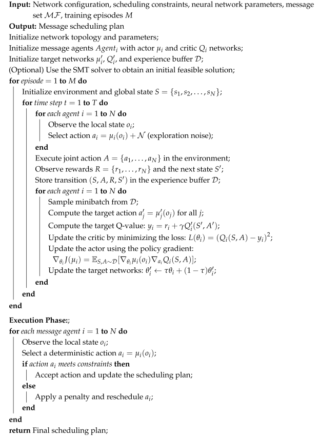
3.3.3. Hybrid Scheduling Algorithm Flow Based on SMT and MADDPG

Multi-agent reinforcement learning is a method of reinforcement learning, and its essence is to explore and try to learn through multiple agents. Therefore, giving some initial experience guidance to agents is conducive to improving training results and speeding up training efficiency. In the MADDPG algorithm, the initial stage of agent training is inefficient in message planning because there is no experience guidance, which leads to a slow execution rate and long consumption time of the algorithm. SMT’s mathematical algorithm has high efficiency in solving message scheduling, but the solution obtained by this algorithm is only feasible, and there is a problem in that it cannot be optimized. Therefore, the feasible solution obtained by SMT mathematical algorithm is taken as the initial accumulated experience of algorithm training, and the scheduling schedule obtained by SMT mathematical algorithm is transformed into the weights in MADPG algorithm, and the weight ratio is adjusted based on the effect of algorithm training, and the obtained basic solution is used to guide MADPG algorithm training.

In the algorithm flow, firstly, the network configuration information, network scheduling constraint parameters and neural network parameters are initialized, and at the same time, the message cluster needs to be initialized. After that, the messages to be scheduled and the conditions to be met are combined into the corresponding formula, and the formula is input into the solver to obtain a feasible solution. Finally, the solution is used as the initial weight value of the algorithm training, and the weight ratio is adjusted based on the effect of the algorithm training.

In the training stage, each message is explored according to the current state S and the strategy selection action a; after each action selection, it is necessary to judge whether the action meets the constraint conditions, and if not, give a negative return value and return to re-schedule; if yes, the reward value r and the state $S^{\prime }$ at the next moment are observed after the action is executed, and the experience vectors $(s,a,s^{\prime },r)$ are stored in the experience pool D to update the state S; by sampling the data in the empirical area D randomly in small batches, and updating the critic network with the sampled data and the loss minimization function, and updating the actor network with the sampled data and the strategic gradient function; after the training is completed, it is necessary to reset the training environment to prevent the next training from being affected by the training results; based on the training effect of the algorithm, the training times of the algorithm are determined.

In the execution stage, the message agent relies on the optimized policy network to guide the agent’s policy network, inputs the local observation $o_i$, and outputs the scheduling action through the operation of the policy network. After each action selection, it is necessary to judge whether the action meets the constraint conditions; if not, it will give a negative return value and restart the message scheduling. After all messages are successfully scheduled, the scheduled result is obtained.

The algorithm flow is described as follows (Algorithm 1):

3.4. Constraint Enforcement in Training and Testing

To ensure that the scheduling process satisfies the constraints defined in Section 2.2 namely periodicity, transmission sequence, and end-to-end delay, we adopt a hybrid enforcement strategy that combines action validation with reward feedback.

During Training (Exploration Phase):

• When an agent selects an action (i.e., chooses an offset time), the action is tentatively applied to the environment.
• All constraints are then checked:
  • Periodicity constraint: Verifies that all message instances fit within their periods.
  • Transmission sequence constraint: Ensures that on each message’s path, downstream links are scheduled after upstream links.
  • End-to-end delay constraint: Calculates the total propagation delay and ensures it is within the allowable limit.
• If the chosen action violates any constraint, the environment rejects the action, gives a negative reward, and the agent is required to reselect an action. This mimics a rescheduling mechanism.
• If the action is feasible, it is accepted and added to the schedule, and a positive or neutral reward is returned depending on success or partial progress.

During Testing (Execution Phase):

• Agents make deterministic decisions using the learned policy network (i.e., select the best offset).
• Each action is immediately checked for constraint satisfaction before being committed to the schedule.
• If the action fails, a retry is triggered using backup rules or heuristic fallback (e.g., greedy slot selection). If the retry fails, the scheduling instance is marked as infeasible.

This approach ensures that constraint violations are not silently ignored, and agents learn both from success and failure during training. The constraint check and feedback mechanism plays a critical role in shaping the reward function landscape and guiding convergence to feasible and efficient scheduling policies.

Algorithm 1:Multi-Agent Message Scheduling Algorithm Based on MADDPG

4. Experimental Verification and Analysis of Algorithm

The main purpose of this paper is to study the feasibility of message scheduling algorithm, so in this experiment, we do not consider the failure of the network due to the failure of network nodes, the redundant processing mechanism in case of failure, and the multi-channel network topology, so the network topology in the experiment is all single-channel network topology. In the network topology, the end system, the switch and the physical link are the same model, and the virtual link, the period and the length of the message to be scheduled are all generated randomly, and the network bandwidth in the environment is set to 1000 Mbps. Among them, the period of time-triggered messages is taken as 1 ms, 2 ms, 4 ms, 8 ms, 16 ms and 32 ms. The bandwidth allocation interval of RC messages is uniformly set to 1 ms. In order to simulate the real network environment, all RC and BE messages are randomly set in the simulation experiment.

Table 1. Time triggered Ethernet message situation table.

Message Number	Message Type	Source Node	Destination Node	Message Period (ms)	Message Length (byte)
1	TT	es0	es5	1	128
2	TT	es0	es3	8	300
3	TT	es2	es6	16	256
···	···	···	···	···	···
5	RC	es3	es6	lack	512
6	RC	es5	es4	lack	200
···	···	···	···	···	···
13	BE	es8	es10	lack	1024
14	BE	es9	es2	lack	100
···	···	···	···	···	···

shows examples of messages.

4.1. Experimental Environment and Performance Metrics

In the previous article, the time-triggered Ethernet message scheduling algorithm is described. After that, the TTE network simulation model based on the OPNET (Optimized Network Engineering Tools) network simulation platform is used to verify the message scheduling algorithm in the simulation network environment. In this experiment, the correctness and efficiency of the proposed method are verified by comparing it with the mathematical solution algorithm based on SMT, and the DQN (Deep Q-Network) algorithm, based on traditional reinforcement learning, is represented by DQN. In all the experiments, the DQN algorithm based on traditional reinforcement learning is represented by DQN, the scheduling algorithm based on MADPG is represented by MADPG, and the hybrid scheduling algorithm based on SMT experience is represented by SMT-MADDPG.

At present, the traditional scheduling algorithm can only obtain a feasible solution for scheduling, but the scheduling effect of event-triggered messages is poor, which will cause a large delay. Therefore, the research goal of this paper is to consider the load balance of scheduling results on the premise of meeting the success of TT message scheduling, and try to prevent the message scheduling from being very tightly arranged in planning, so as to obtain a better solution for event-triggered message scheduling.

Another index of experimental verification is to calculate the end-to-end delay of RC and BE messages in the network for different algorithms in the OPNET network simulation environment.

The total end-to-end delay of RC messages in the network can be expressed by the average end-to-end delay of each RC message:

$$ED\_AL{L}^{RC}=\sum _{i=1}^S\left(E{D}_i^{RC}\right)/S$$

(16)

where $ED\_AL{L}^{RC}$ represents the total end-to-end delay of RC messages in the whole network, S represents the number of RC messages in the network, and $E{D}_i^{RC}$ represents the end-to-end delay of the ith RC message.

The total end-to-end delay of BE messages in the network can be expressed by the average end-to-end delay of each BE message:

$$ED\_AL{L}^{BE}=\sum _{j=1}^W\left(E{D}_j^{BE}\right)/W$$

(17)

where $ED\_AL{L}^{BE}$ represents the total end-to-end delay of BE messages in the whole network, W represents the number of BE messages in the network, and $E{D}_j^{BE}$ represents the end-to-end delay of the j-th BE message.

According to the above two formulas, when the scheduling result has a solution, the total end-to-end delay of RC and BE messages in the message scheduling result is taken as the final index to judge the scheduling result.

In this experiment, there are four groups. The first two groups of experiments have the same network topology, which is the A380 switching architecture topology, but the number of messages is different, and the numbers are Experiment 1 and Experiment 2, respectively. The network topology of the last two groups of experiments is an extended star network topology, and the number of messages is also different, with the numbers being Experiment 3 and Experiment 4, respectively.

4.2. Extended Evaluation Metrics

In addition to the average end-to-end delay and load balance metrics already described, the following additional evaluation indicators are introduced to comprehensively assess the performance of different scheduling algorithms:

• Jitter of RC/BE Messages: Jitter is defined as the variation in the end-to-end delay of a message type. Specifically, for RC and BE messages, we compute both the maximum delay difference and the standard deviation:

  $${\mathrm{Jitter}}_{RC}=max\left(D_{RC}\right)-min\left(D_{RC}\right),{\sigma }_{RC}=\mathrm{std}\left(D_{RC}\right)$$
  Lower jitter implies more consistent message delivery, which is crucial in real-time and critical systems.
• Computation Time: The total time required by each algorithm to produce a complete feasible schedule, measured in seconds. This metric reflects algorithmic efficiency and practicality in real deployment.
• Feasibility Rate: For a fixed scheduling time window (e.g., 5 s), the percentage of scheduling attempts that successfully generate a valid schedule. This measures robustness under time constraints.
• (Optional) Training Convergence Steps: For MARL-based methods, we record the number of episodes required for training loss and reward to stabilize. This indicates training efficiency.

These additional metrics provide deeper insights into each algorithm’s consistency, efficiency, and robustness beyond average-case performance.

4.3. A380 Switching Architecture Topology Environment

The first network topology in this experiment uses A380 switching architecture topology.

The experimental network topology is shown in Figure 7, which consists of 8 switches, 16 end systems and 31 physical links.

4.3.1. Experiment 1

In MADDPG, the learning rate of the Actor network needs to be higher than that of the Critic network to avoid premature convergence of the strategy. According to the following empirical formula: ${\alpha }_{\mathrm{actor}}=2\times {\alpha }_{\mathrm{critic}}$.

In the experiment, Critic network uses ${\alpha }_{\mathrm{critic}}$ = 0.375, so ${\alpha }_{\mathrm{actor}}$ = 0.75.

The discount factor should reflect the timeliness requirements of event-triggered messages. Assuming that the maximum tolerated delay of the BE message is ${\tau }_{\max }$ = 10 ms, then $\gamma =e^{-{\displaystyle \frac{T_{\mathrm{step}}}{{\tau }_{\max }}}}=e^{-{\displaystyle \frac{1\mathrm{ms}}{10\mathrm{ms}}}}\approx 0.905$ (Take $\gamma$ = 0.85 to enhance short-term rewards.)

In Experiment 1, there are 84 TT messages, and the total hop count of the messages passing through the switch is 272 hops. The hypercycle of the messages in the network is 8000 us, so 1037 message frames are generated in a hypercycle. At the same time, the network also contains 313 RC messages and 295 BE messages. The training times of the algorithm are set to 50,000 times, the learning efficiency A is set to 0.75, the attenuation factor R is set to 0.85, and the network update rate is set to 0.2. All the above parameters are set by debugging in the experiment.

Figure 8 shows the local load balance of TT message scheduling on a certain link when four methods are successfully scheduled. As can be seen from the figure, the scheduling algorithm based on SMT closely arranges all TT messages together, and the scheduling algorithm based on DQN disperses TT messages, while the scheduling algorithms based on MADPG and SMT-MADDPG have better load balance than the scheduling algorithms based on SMT and DQN.

From

Table 2. Experiment 1: Load balance value of scheduling results of four algorithms.

Algorithm Name	SMT	DQN	MADDPG	SMT-MADDPG
Load balance value	447.23	351.09	264.47	253.93

, it can be seen that the load balance value of the scheduling results of the algorithm based on multi-agent reinforcement learning is obviously better than that of the scheduling algorithms based on SMT and DQN. In this experiment, the load balance of the scheduling algorithm based on SMT is the worst because the algorithm can only find the feasible solution of scheduling, and does not pay attention to the balance of scheduling messages, which is only related to the network topology environment. The scheduling method based on DQN is second; the effect based on MADDPG is basically the same as that based on SMT-MADDPG.

As can be seen from Figure 9 and Figure 10 and

Table 3. Experiment 1: The results of four algorithms show the end-to-end delay mean of RC and BE messages.

Algorithm Name	SMT	DQN	MADDPG	SMT-MADDPG
Average total delay of RC messages/us	7079.73	6715.398	6463.93	6436.541
Average total delay of BE messages/us	7328.473	6741.175	6509.499	6379.999

, the scheduling algorithm based on multi-agent reinforcement learning has a significantly lower delay in scheduling RC and BE messages than the scheduling algorithm based on SMT and DQN. In this experiment, the message delay based on SMT is the largest. Because of the limitation of the SMT algorithm itself, it only seeks a feasible solution, so it will not actively leave time slots for RC and BE messages. The scheduling algorithm based on DQN is second; the scheduling algorithm based on SMT-MADDPG has the lowest delay for RC and BE in this experiment.

4.3.2. Experiment 2

In Experiment 2, the size of messages in the network is improved. There are 162 TT messages in the network, and the total hop count of messages transferred through the switch is 532 hops. The hypercycle of messages in the network is 16,000 us, so 2035 scheduling message frames are generated in a hypercycle. At the same time, the network also contains 407 RC messages and 389 BE messages. The training times of the algorithm are set to 100,000 times, the learning efficiency A is set to 0.75, the attenuation factor R is set to 0.85, and the network update rate T is set to 0.2. All the above parameters are set by debugging in the experiment.

As can be seen from Figure 11, the scheduling algorithm based on SMT only obtains feasible solutions, and arranges TT messages relatively closely together; the scheduling algorithm based on DQN is more discrete than that based on SMT. The scheduling algorithm based on multi-agent reinforcement learning is better than the SMT-based scheduling algorithm and the DQN-based scheduling algorithm in the load balance of message scheduling results.

Table 4. Experiment 2: Load balance value of scheduling results of four algorithms.

Algorithm Name	SMT	DQN	MADDPG	SMT-MADDPG
Load balance value	512.48	396.35	282.85	285.61

records the global message load of the different scheduling methods. In Table 4, it can be seen that the load balance value of scheduling results based on multi-agent reinforcement learning algorithm is obviously better than that based on SMT and DQN. In this experiment, the load balance based on the SMT scheduling algorithm is the worst. The method based on DQN is the second; the scheduling algorithm based on MADDPG performs best in load balancing.

As can be seen from Figure 12 and Figure 13 and

Table 5. Experiment 2 The results of four algorithms show the end-to-end delay mean of RC and BE messages.

Algorithm Name	SMT	DQN	MADDPG	SMT-MADDPG
Average total delay of RC messages/us	9655.802	8909.369	8547.994	8620.129
Average total delay of BE messages/us	10,094.38	9219.712	8960.095	9031.741

, the scheduling algorithm based on multi-agent reinforcement learning has a significantly lower scheduling delay for RC and BE messages than that based on SMT and DQN, and the message delay based on SMT is the largest in this experiment. The scheduling algorithm based on MADDPG has the lowest delay for RC and BE in this experiment.

4.4. Extended Star Network Topology Environment

The extended star network topology is centered with multiple switches connected, and then connected to multiple end systems. The extended star network in this experiment consists of 16 end systems, 4 switches and 20 physical links. The extended star network topology is shown in Figure 14.

4.4.1. Experiment 3

In Experiment 3, there are 90 messages to be scheduled in the network, and the total number of hops of messages transferred through the switch is 231. The hypercycle of messages in the network is 16,000 us, so 996 scheduling message frames are generated in one hypercycle. At the same time, the network also contains 297 RC messages and 302 BE messages. The training times of the algorithm are set to 80,000 times, the learning efficiency A is set to 0.75, the attenuation factor R is set to 0.85, the network update rate T is set to 0.2, and the parameters are set by debugging.

Figure 15 shows the local load balancing of TT message scheduling by different algorithms on a link under the premise of successful scheduling. According to the analysis of the above figure, the TT messages obtained by the SMT-based scheduling algorithm are closely arranged; the scheduling algorithm based on DQN distributes TT messages more discretely; the scheduling algorithm based on multi-agent reinforcement learning is superior to the SMT-based scheduling algorithm and the DQN-based scheduling algorithm in the load balance of message scheduling results.

As can be seen from

Table 6. Experiment 3 Load balance value of scheduling results of four algorithms.

Algorithm Name	SMT	DQN	MADDPG	SMT-MADDPG
Load balance value	1472.65	683.91	354.26	342.87

, the load balancing of the scheduling algorithm based on SMT-MADDPG is the best in this experiment. For the average load of each sub-link in the scheduling slot, the load balance value of the scheduling algorithm based on multi-agent reinforcement learning is close, which is better than that of the scheduling algorithm based on SMT and DQN.

As can be seen from Figure 16 and Figure 17 and

Table 7. Experiment 3: The results of four algorithms show the end-to-end delay mean of RC and BE messages.

Algorithm Name	SMT	DQN	MADDPG	SMT-MADDPG
Average total delay of RC messages/us	20,167.78	19,127.4	18,466.39	18,357.35
Average total delay of BE messages/us	30,982.99	29,100.03	28,365.02	28,151.77

, the scheduling algorithm based on multi-agent reinforcement learning has a significantly lower delay in scheduling RC and BE messages than the scheduling algorithm based on SMT and DQN, and the message delay based on SMT is the largest in this experiment. The algorithm based on MADDPG is at the same level as that based on SMT-MADDPG, and the scheduling algorithm based on SMT-MADDPG has the lowest delay for RC and BE in this experiment.

4.4.2. Experiment 4

In Experiment 4, there are 190 TT messages in the network, and the total number of hops of messages passing through the switch is 516, and the hypercycle of messages in the network is 32,000 us, so 6,929 message frames are generated in one hypercycle. At the same time, the network also contains 399 RC messages and 410 BE messages. The training times of the algorithm are set to 150,000 times, the learning efficiency A is set to 0.75, the attenuation factor R is set to 0.85, and the network update rate T is set to 0.2. All the above parameters are set by debugging in the experiment.

As shown in Figure 18 above, the scheduling algorithm based on SMT arranges TT messages closely. The scheduling algorithm based on DQN arranges TT messages in a scattered way; the scheduling algorithm based on multi-agent reinforcement learning is superior to the scheduling algorithm based on SMT and the scheduling algorithm based on DQN in the case of uniform message scheduling.

As can be seen from

Table 8. Experiment 4: Load balance value of scheduling results of four algorithms.

Algorithm Name	SMT	DQN	MADDPG	SMT-MADDPG
Load balance value	975.30	515.39	378.50	361.52

, the load balancing of the scheduling algorithm based on SMT-MADDPG is the best in this experiment. For the average load of each sub-link in the scheduling time slot, the load balance value of the scheduling algorithm based on multi-agent reinforcement learning is similar, which is better than that of the scheduling algorithm based on SMT and DQN.

As can be seen from Figure 19 and Figure 20 and

Table 9. Experiment 4: The results of four algorithms show the end-to-end delay mean of RC and BE messages.

Algorithm Name	SMT	DQN	MADDPG	SMT-MADDPG
Average total delay of RC messages/us	41,301.09	38,667.44	37,533.56	37,412.93
Average total delay of BE messages/us	55,452.75	52,454.93	51,079.61	50,564.32

, the scheduling algorithm based on multi-agent reinforcement learning has a significantly lower delay in scheduling RC and BE messages than the scheduling algorithm based on SMT and DQN, and the message delay based on SMT is the largest in this experiment. The algorithm based on MADDPG is at the same level as that based on SMT-MADDPG, and the scheduling algorithm based on SMT-MADDPG has the lowest delay for RC and BE in this experiment.

5. Conclusions

In this paper, a message scheduling algorithm based on multi-agent reinforcement learning (MADDPG) is proposed. Through centralized training and distributed execution, combined with a global information guidance strategy network training, the scheduling of event-triggered messages is optimized. This paper also introduces the SMT mathematical method to accelerate the convergence of the MADDPG algorithm and form a hybrid algorithm. Experiments show that the algorithm achieves better load balancing compared with SMT and DQN algorithms under the A380 switching architecture and extended star network topology. In addition, the TTE message scheduling planning software is developed to verify the effectiveness of the algorithm. Future work will focus on improving algorithm efficiency, optimizing TT message distribution, and enhancing adaptability in different network environments.

References

1. Obermaisser, R. Time-Triggered Communication; CRC Press: Boca Raton, FL, USA, 2012; Volume 19. [Google Scholar]
2. Calabrese, M.; Curbo, J.; Falco, G. A Software Defined Networking Architecture for Time Triggered Ethernet in Space Systems. In Proceedings of the 2024 IEEE International Conference on Wireless for Space and Extreme Environments (WiSEE), Daytona Beach, FL, USA, 16–18 December 2024; IEEE: Piscataway, NJ, USA, 2024; pp. 207–212. [Google Scholar]
3. Kopetz, H.; Bauer, G. The time-triggered architecture. Proc. IEEE 2003, 91, 112–126. [Google Scholar] [CrossRef]
4. Kopetz, H.; Grunsteidl, G. TTP-A time-triggered protocol for fault-tolerant real-time systems. In Proceedings of the FTCS-23 the Twenty-Third International Symposium on Fault-Tolerant Computing, Toulouse, France, 22–24 June 1993; IEEE: Piscataway, NJ, USA, 1993; pp. 524–533. [Google Scholar]
5. Li, Z.; Wan, H.; Pang, Z.; Chen, Q.; Deng, Y.; Zhao, X.; Gao, Y.; Song, X.; Gu, M. An enhanced reconfiguration for deterministic transmission in time-triggered networks. IEEE/ACM Trans. Netw. 2019, 27, 1124–1137. [Google Scholar] [CrossRef]
6. Steiner, W. An evaluation of SMT-based schedule synthesis for time-triggered multi-hop networks. In Proceedings of the 2010 31st IEEE Real-Time Systems Symposium, San Diego, CA, USA, 30 November–3 December 2010; IEEE: Piscataway, NJ, USA, 2010; pp. 375–384. [Google Scholar]
7. Pozo, F.; Rodriguez-Navas, G.; Hansson, H. Methods for large-scale time-triggered network scheduling. Electronics 2019, 8, 738. [Google Scholar] [CrossRef]
8. Trüb, R.; Giannopoulou, G.; Tretter, A.; Thiele, L. Implementation of partitioned mixed-criticality scheduling on a multi-core platform. ACM Trans. Embed. Comput. Syst. (TECS) 2017, 16, 1–21. [Google Scholar] [CrossRef]
9. Xuan, Z.; Xiong, H.; Feng, H. Hybrid partition-and network-level scheduling design for distributed integrated modular avionics systems. Chin. J. Aeronaut. 2020, 33, 308–323. [Google Scholar]
10. Rashid, T.; Samvelyan, M.; De Witt, C.S.; Farquhar, G.; Foerster, J.; Whiteson, S. Monotonic value function factorisation for deep multi-agent reinforcement learning. J. Mach. Learn. Res. 2020, 21, 1–51. [Google Scholar]
11. Miyazaki, K.; Matsunaga, N.; Murata, K. Formation path learning for cooperative transportation of multiple robots using MADDPG. In Proceedings of the 2021 21st International Conference on Control, Automation and Systems (ICCAS), Jeju, Republic of Korea, 12–15 October 2021; IEEE: Piscataway, NJ, USA, 2021; pp. 1619–1623. [Google Scholar]
12. Lei, W.; Wen, H.; Wu, J.; Hou, W. MADDPG-based security situational awareness for smart grid with intelligent edge. Appl. Sci. 2021, 11, 3101. [Google Scholar] [CrossRef]
13. Jiang, M.; Hai, T.; Pan, Z.; Wang, H.; Jia, Y.; Deng, C. Multi-agent deep reinforcement learning for multi-object tracker. IEEE Access 2019, 7, 32400–32407. [Google Scholar] [CrossRef]
14. Novati, G.; de Laroussilhe, H.L.; Koumoutsakos, P. Automating turbulence modelling by multi-agent reinforcement learning. Nat. Mach. Intell. 2021, 3, 87–96. [Google Scholar] [CrossRef]
15. Li, C.; Fussell, L.; Komura, T. Multi-agent reinforcement learning for character control. Vis. Comput. 2021, 37, 3115–3123. [Google Scholar] [CrossRef]
16. Zhao, C.; Zhang, X.; Li, X.; Du, Y. Intelligent delay matching method for parking allocation system via multi-agent deep reinforcement learning. China J. Highw. Transp. 2022, 35, 261–272. [Google Scholar]
17. Dong, L.; Liu, Y.; Qiao, J.; Wang, X.; Wang, C.; Pu, T. Optimal dispatch of combined heat and power system based on multi-agent deep reinforcement learning. Power Syst. Technol. 2021, 45, 4729–4738. [Google Scholar]
Figure 1. Time triggered network topology.
Electronics 14 02575 g001
Figure 2. Hybrid topology.
Electronics 14 02575 g002
Figure 3. Schematic diagram of scheduling success status.
Electronics 14 02575 g003
Figure 4. Schematic diagram of scheduling failure state.
Electronics 14 02575 g004
Figure 5. Schematic diagram of TT, RC and BE scheduling results.
Electronics 14 02575 g005
Figure 6. Link load.
Electronics 14 02575 g006
Figure 7. A380 network topology architecture.
Electronics 14 02575 g007
Figure 8. Local load balancing diagram of messages of different algorithms on a link.
Electronics 14 02575 g008
Figure 9. In experiment 1, the end-to-end delay of RC messages in the simulation environment is analyzed.
Electronics 14 02575 g009
Figure 10. In experiment 1, the end-to-end delay of BE messages in the simulation environment is analyzed.
Electronics 14 02575 g010
Figure 11. Load balance diagram of different algorithms at the moment of transmission on a link.
Electronics 14 02575 g011
Figure 12. In Experiment 2, the end-to-end delay of RC messages in the simulation environment is analyzed.
Electronics 14 02575 g012
Figure 13. In experiment 2, the end-to-end delay of BE messages in the simulation environment is analyzed.
Electronics 14 02575 g013
Figure 14. Extended star network topology environment diagram.
Electronics 14 02575 g014
Figure 15. Load balance diagram of different algorithms at the moment of transmission on a link.
Electronics 14 02575 g015
Figure 16. In Experiment 3, the end-to-end delay of RC messages in the simulation environment is analyzed.
Electronics 14 02575 g016
Figure 17. In Experiment 3, the end-to-end delay of BE messages in the simulation environment is analyzed.
Electronics 14 02575 g017
Figure 18. Load balance diagram of different algorithms at the moment of transmission on a link.
Electronics 14 02575 g018
Figure 19. In Experiment 4, the end-to-end delay of RC messages in the simulation environment is analyzed.
Electronics 14 02575 g019
Figure 20. In Experiment 4, the end-to-end delay of BE messages in the simulation environment is analyzed.
Electronics 14 02575 g020