
Explainable AI Models for IoT-Based Shaft Power Prediction and Comprehensive Performance Monitoring

 , , , , ,
Abstract
1. Introduction
- Pioneering the application of explainable machine learning algorithms for shaft power prediction, shedding light on the decision-making process and enhancing transparency in model outputs.
- Applying explainable AI methods to offer a deeper understanding of how shaft power predictions affect fuel usage and emissions. This contributes to more transparent and actionable insights for monitoring and controlling emissions, thereby improving environmental compliance and performance tracking.
- Pioneering the use of machine learning algorithms to predict shaft power and optimize operational parameters, which helps in reducing fouling rates by maintaining consistent and efficient engine performance. This approach aids in minimizing the frequency and impact of fouling-related maintenance, thereby enhancing vessel efficiency.
- Conducting a comprehensive comparative analysis between machine learning methods and current industry practices for shaft power prediction, offering insights into the potential improvements and advancements achievable through novel approaches.
- The recommended method can be embedded in a system that enables real-time monitoring of shaft power and performance parameters. Additionally, the system can promptly alert operators to anomalies or deviations from expected performance, allowing for quick intervention and correction.
2. Related Work

| Literature | Methods | Prediction |
|---|---|---|
| [20] | LR | Shaft Power |
| [18] | XGBoost | Ship Propulsion Power |
| [15] | ANN | Shaft Power |
| [16] | ANN | Shaft Power |
| [22] | MLR | Fuel Consumption |
| [23] | LGBM | Fuel Consumption |
| [21] | Ensemble NN, ANN | Shaft Power |
| [24] | ANN | Shaft Power |
| [25] | SVM | Misalignment defects detection |
| [26] | MLR, DT, K-NN ANN, RF | Shaft Power |
| [27] | RNN, CNN | Power Output of Turbines |
| [28] | RF | Shaft Power |
| [29] | MLR, Ridge, LASSO SVR, Tree-Based Algorithms. | Fuel Consumption |
| [30] | ANN, GPR | Fuel Consumption |
| [31] | ANN, MLR | Fuel Consumption |
| [17] | CNN | Hull Form Performance |
| [32] | ANN | Ship Speed Fuel Consumption |
| [33] | SVM, RFR, ETR, ANN | Fuel Consumption |
3. Tools and Methods
3.1. Dataset
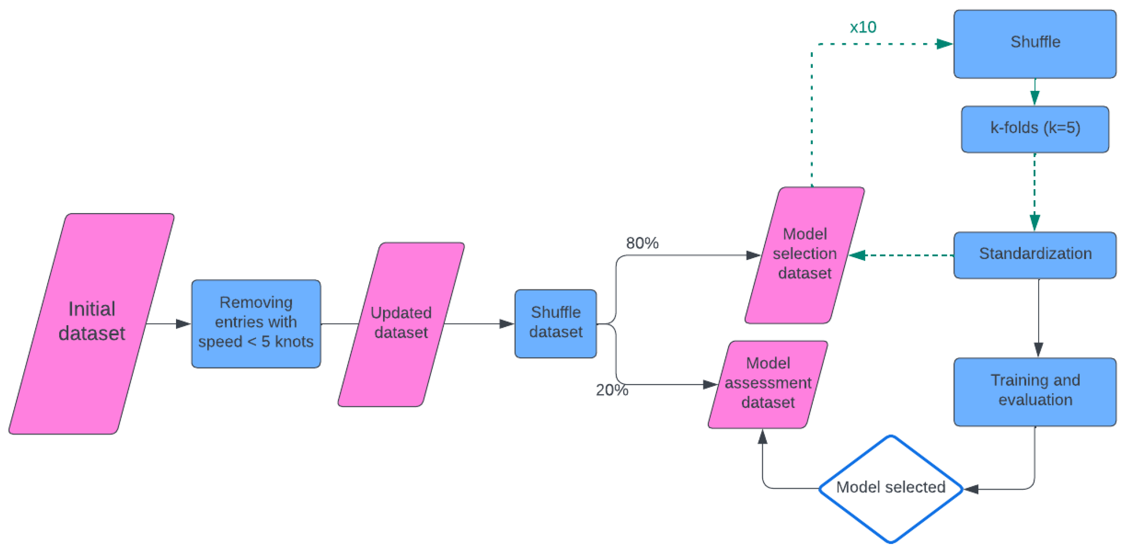
3.2. Methodology
3.3. Standardization
3.4. Machine Learning Algorithms
3.4.1. k-Nearest Neighbors
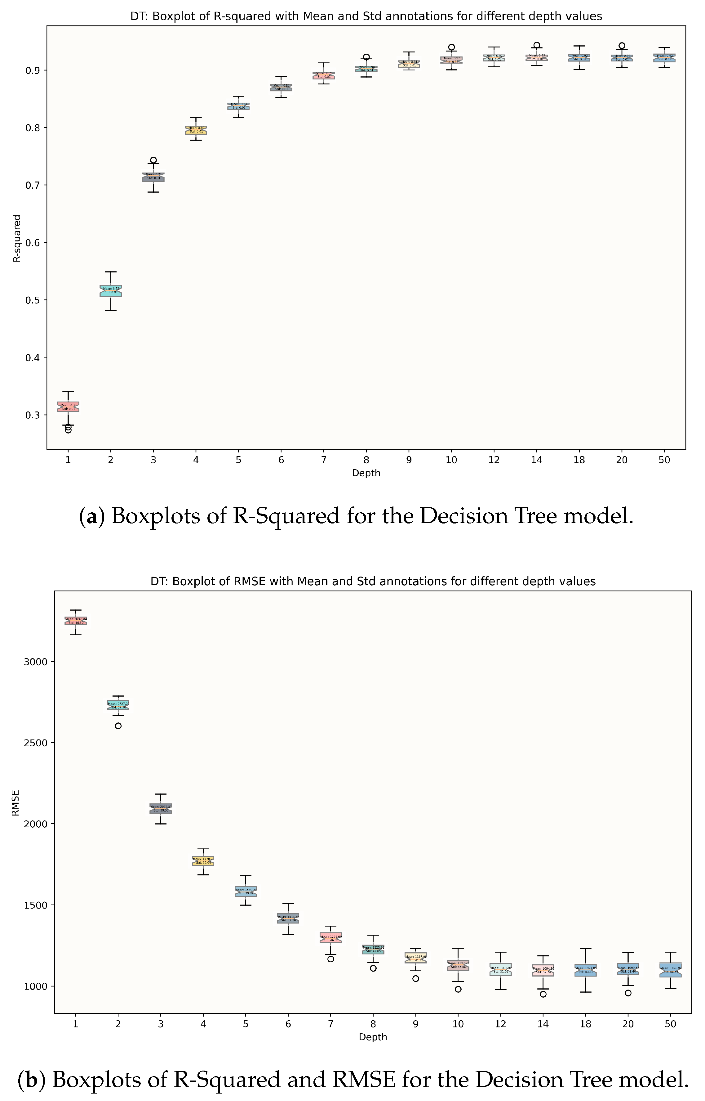
3.4.2. Decision Trees
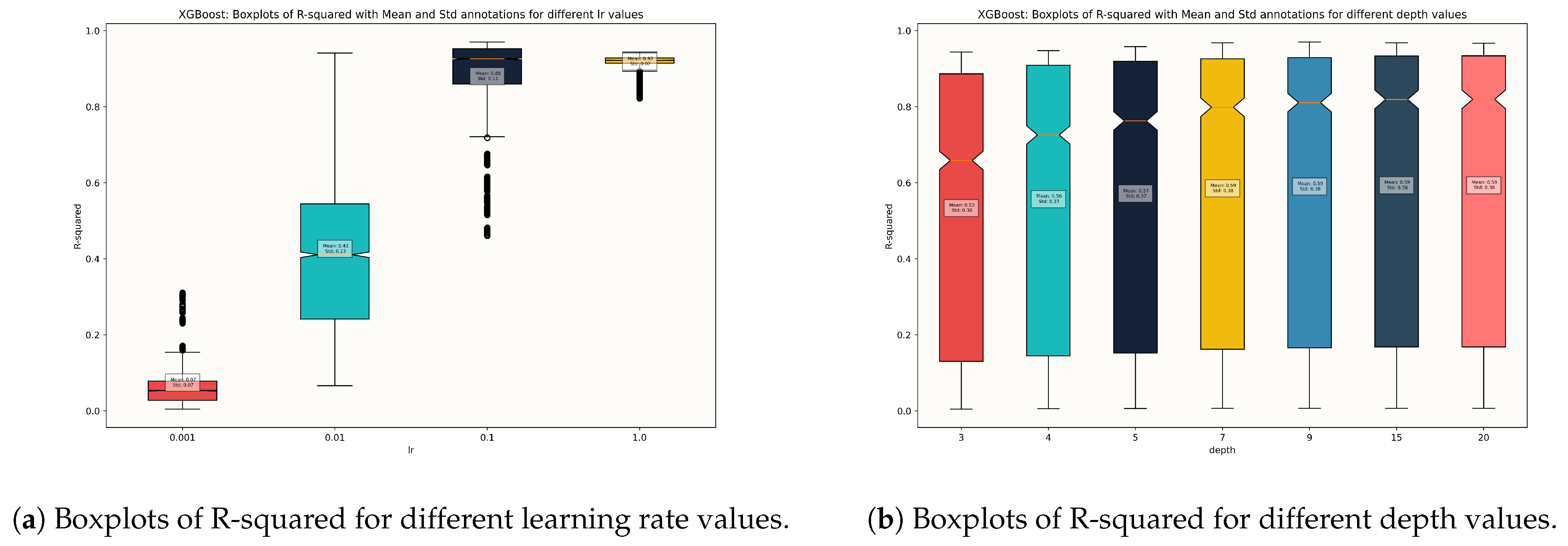
3.4.3. XGBoost
3.5. SHapley Additive exPlanations (SHAP)
3.6. Emissions Estimation Methodology
- is the estimated emission output (e.g., CO2, NOx),
- is the emission factor specific to the pollutant and fuel type (e.g., gCO2/kWh),
- is the total power output of the main engine during the operation period (in kWh).
- shaftpower is the average shaft power delivered by the engine during the voyage (in kW),
- workingtime is the total engine operating time over the analyzed period (in hours).
4. Results
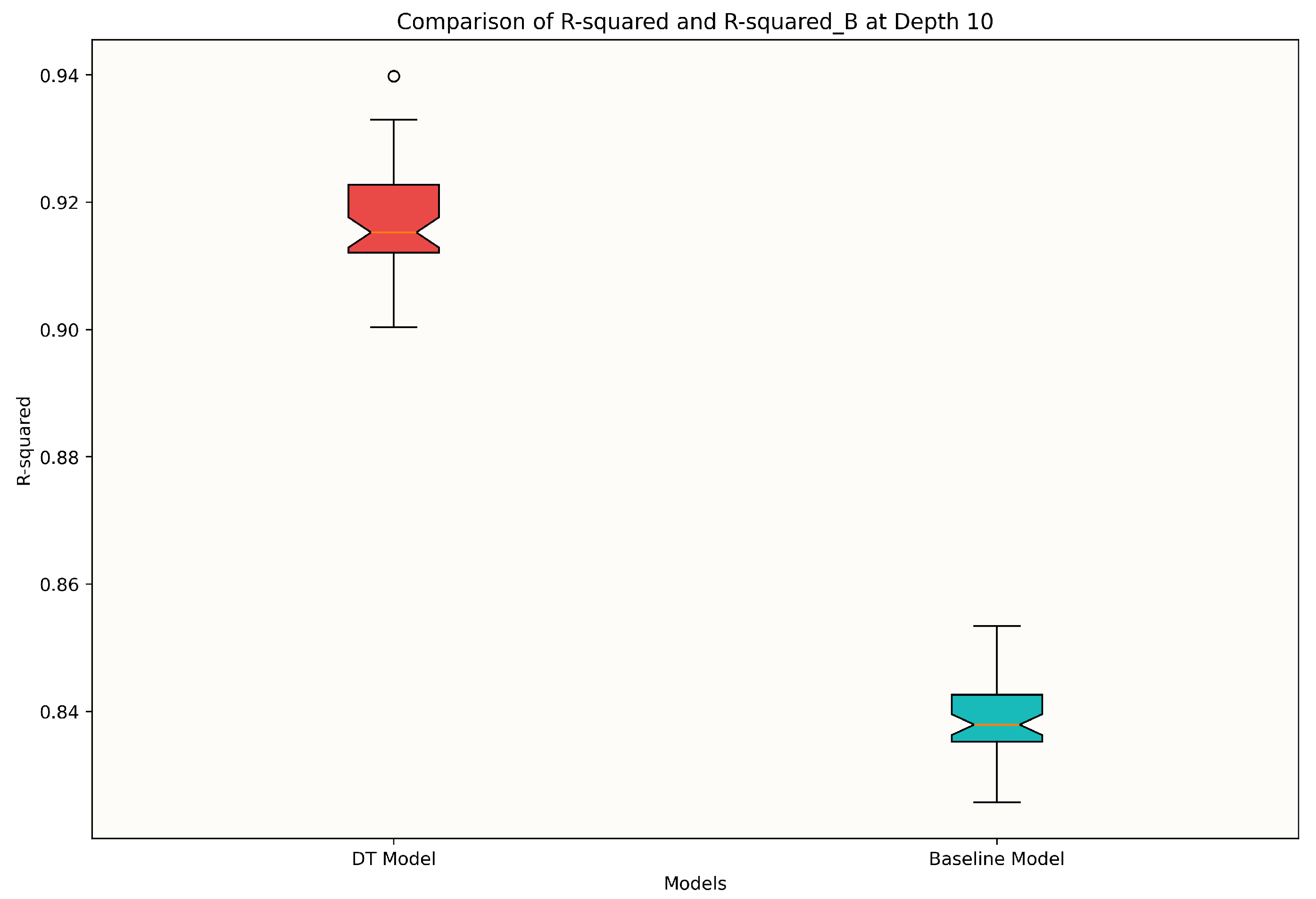
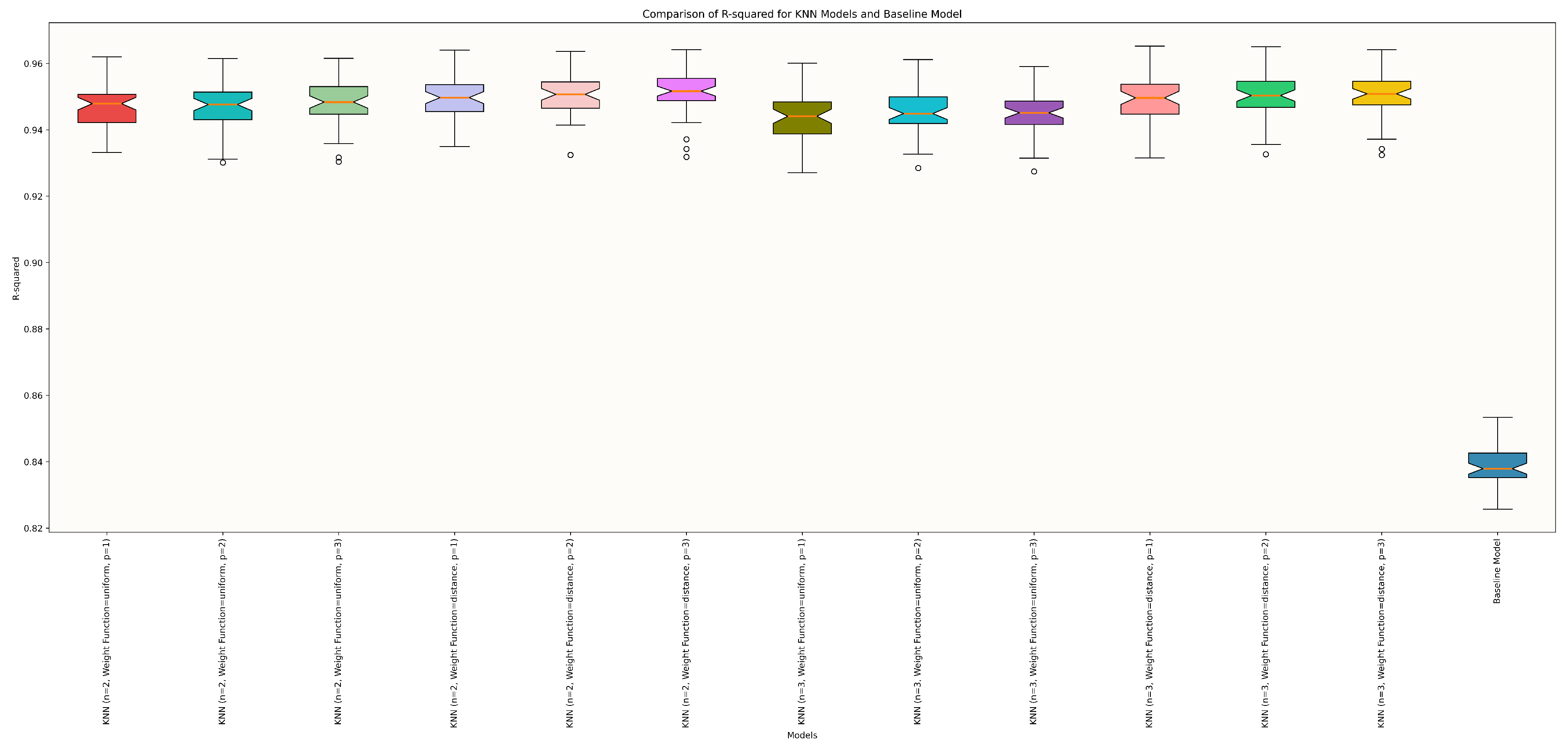
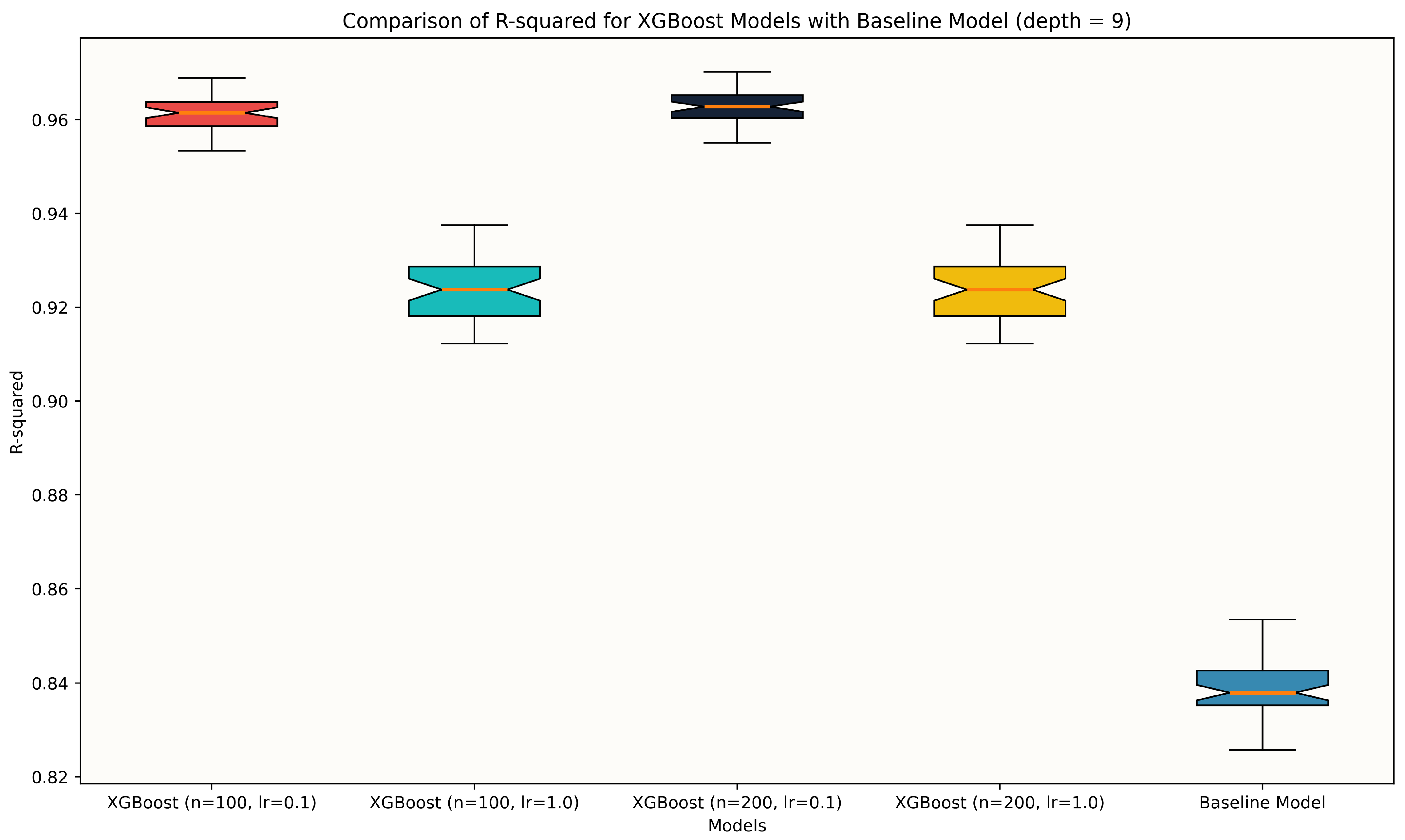
4.1. Model Selection
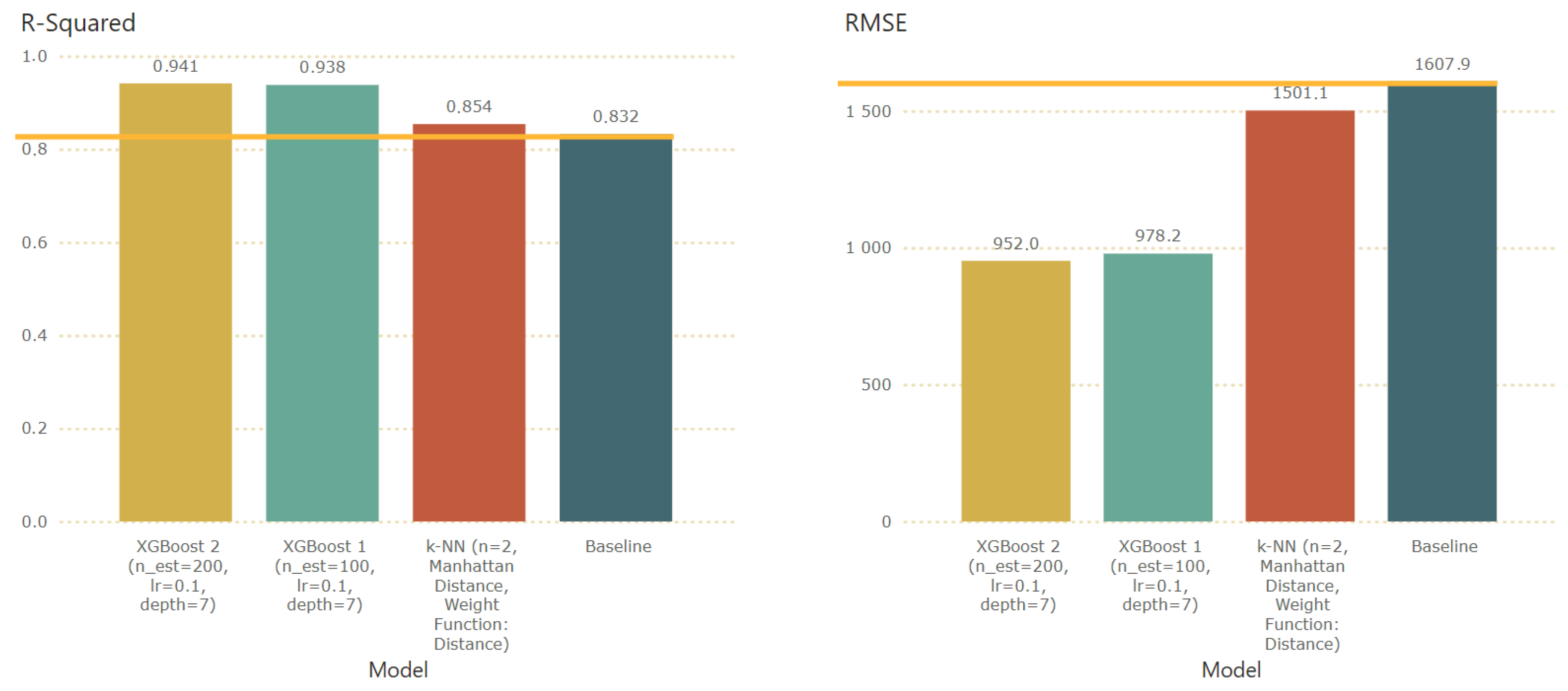
4.2. Model Assessment
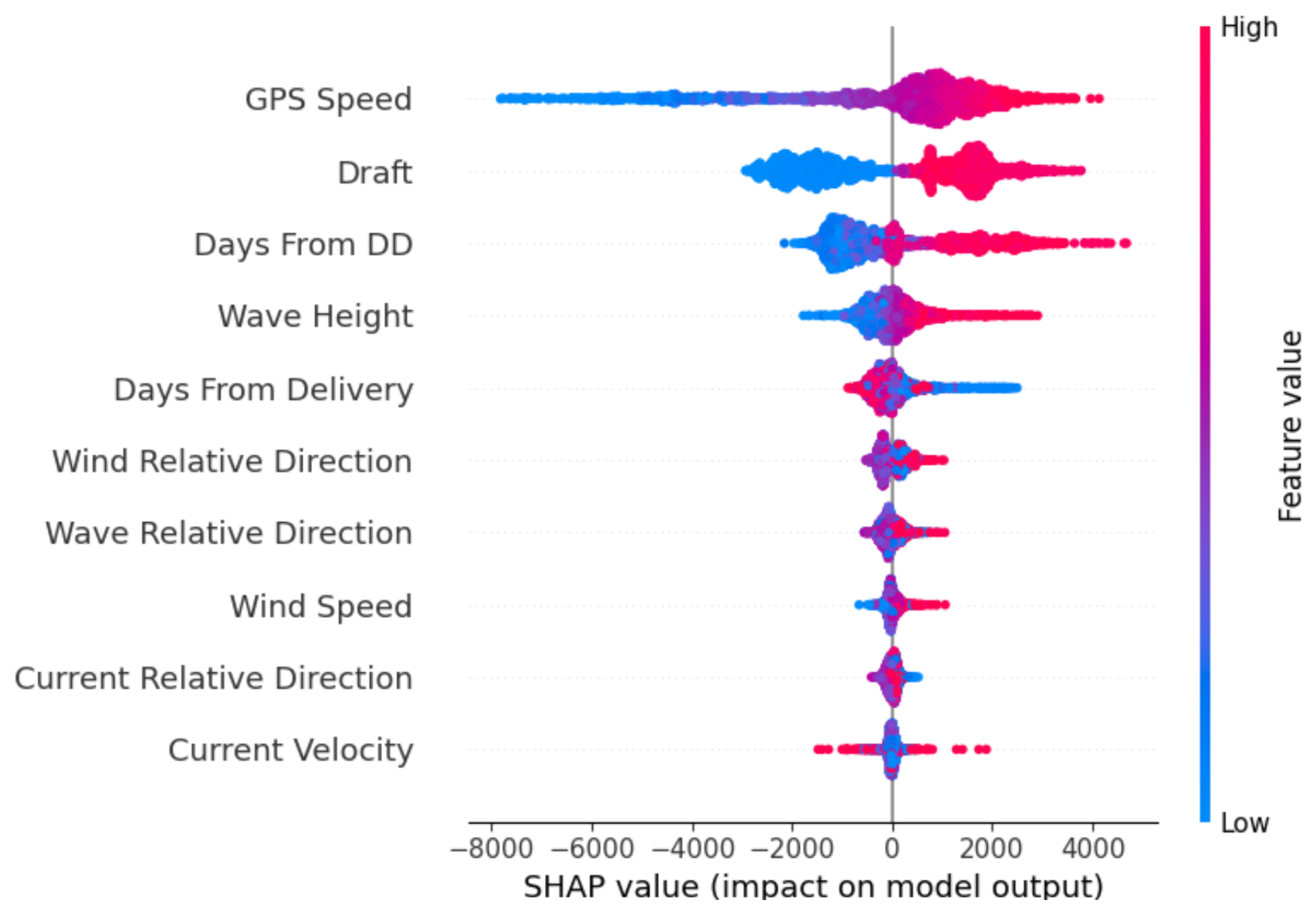
4.3. Explainable Machine Learning with SHAP Framework
5. Discussion
6. Conclusions
Author Contributions
Funding
Data Availability Statement
Conflicts of Interest
Abbreviations
| AI | Artificial Intelligence |
| ANN | Artificial Neural Network |
| API | Application Programming Interface |
| DT | Decision Tree |
| EU | European Union |
| EU ETS | European Union Emissions Trading System |
| IMO | International Maritime Organization |
| IoT | Internet of Things |
| k-NN | k-Nearest Neighbors |
| ML | Machine Learning |
| NN | Neural Network |
| RF | Random Forest |
| RMSE | Root Mean Square Error |
| SHAP | SHapley Additive exPlanations |
| SVM | Support Vector Machine |
| VLCC | Very Large Crude Carrier |
| XAI | Explainable Artificial Intelligence |
| XGBoost | eXtreme Gradient Boosting |
References
- European Commision. Reducing Emissions from the Shipping Sector; European Commision: Brussels, Belgium, 2023. [Google Scholar]
- International Maritime Organization (IMO). 2023 IMO Strategy on Reduction of GHG Emissions from Ships; International Maritime Organization (IMO): London, UK, 2023. [Google Scholar]
- International Maritime Organization (IMO). 2021 Guidelines on the Shaft/Engine Power Limitation System to Comply with the EEXI Requirements and Use of a Power Reserve; International Maritime Organization (IMO): London, UK, 2021. [Google Scholar]
- Gupta, P.; Rasheed, A.; Steen, S. Ship performance monitoring using machine-learning. Ocean Eng. 2022, 254, 111094. [Google Scholar] [CrossRef]
- Fahrnholz, S.F.; Caprace, J.D. A machine learning approach to improve sailboat resistance prediction. Ocean Eng. 2022, 257, 111642. [Google Scholar] [CrossRef]
- Aizpurua, J.I.; Knutsen, K.E.; Heimdal, M.; Vanem, E. Integrated machine learning and probabilistic degradation approach for vessel electric motor prognostics. Ocean Eng. 2023, 275, 114153. [Google Scholar] [CrossRef]
- Panagiotakopoulos, T.; Filippopoulos, I.; Filippopoulos, C.; Filippopoulos, E.; Lajic, Z.; Violaris, A.; Chytas, S.P.; Kiouvrekis, Y. Vessel’s trim optimization using IoT data and machine learning models. In Proceedings of the 2022 13th International Conference on Information, Intelligence, Systems & Applications (IISA), Corfu, Greece, 18–20 July 2022; pp. 1–5. [Google Scholar] [CrossRef]
- Guo, B.; Gupta, P.; Steen, S.; Tvete, H.A. Evaluating vessel technical performance index using physics-based and data-driven approach. Ocean Eng. 2023, 286, 115402. [Google Scholar] [CrossRef]
- Graf von Westarp, A. A new model for the calculation of the bunker fuel speed–consumption relation. Ocean Eng. 2020, 204, 107262. [Google Scholar] [CrossRef]
- Filippopoulos, I.; Panagiotakopoulos, T.; Skiadas, C.; Triantafyllou, S.M.; Violaris, A.; Kiouvrekis, Y. Live Vessels’ Monitoring using Geographic Information and Internet of Things. In Proceedings of the 2022 13th International Conference on Information, Intelligence, Systems & Applications (IISA), Corfu, Greece, 18–20 July 2022; pp. 1–7. [Google Scholar] [CrossRef]
- Liu, S.; Papanikolaou, A.; Shang, B. Regulating the safe navigation of energy-efficient ships: A critical review of the finalized IMO guidelines for assessing the minimum propulsion power of ships in adverse conditions. Ocean Eng. 2022, 249, 111011. [Google Scholar] [CrossRef]
- Li, X.; Sun, B.; Jin, J.; Ding, J. Ship speed optimization method combining Fisher optimal segmentation principle. Appl. Ocean Res. 2023, 140, 103743. [Google Scholar] [CrossRef]
- Hua, R.; Yin, J.; Wang, S.; Han, Y.; Wang, X. Speed optimization for maximizing the ship’s economic benefits considering the Carbon Intensity Indicator (CII). Ocean Eng. 2024, 293, 116712. [Google Scholar] [CrossRef]
- Issa, M.; Ilinca, A.; Martini, F. Ship Energy Efficiency and Maritime Sector Initiatives to Reduce Carbon Emissions. Energies 2022, 15, 7910. [Google Scholar] [CrossRef]
- Delgado-Currín, R.; Calderon-Munoz, W.R.; Elicer-Cortos, J.C. Artificial Neural Network Model for Estimating the Pelton Turbine Shaft Power of a Micro-Hydropower Plant under Different Operating Conditions. Energies 2024, 17, 3597. [Google Scholar] [CrossRef]
- Kriezis, A.C.; Sapsis, T.; Chryssostomidis, C. Predicting Ship Power Using Machine Learning Methods. In Proceedings of the SNAME Maritime Convention, Houston, TX, USA, 27–29 September 2022. [Google Scholar] [CrossRef]
- Kim, Y.C.; Kim, K.S.; Yeon, S.; Lee, Y.Y.; Kim, G.D.; Kim, M. Power Prediction Method for Ships Using Data Regression Models. J. Mar. Sci. Eng. 2023, 11, 1961. [Google Scholar] [CrossRef]
- Lang, X.; Wu, D.; Mao, W. Comparison of supervised machine learning methods to predict ship propulsion power at sea. Ocean Eng. 2022, 245, 110387. [Google Scholar] [CrossRef]
- Valchev, I.; Coraddu, A.; Kalikatzarakis, M.; Geertsma, R.; Oneto, L. Numerical methods for monitoring and evaluating the biofouling state and effects on vessels hull and propeller performance: A review. Ocean Eng. 2022, 251, 110883. [Google Scholar] [CrossRef]
- Kim, H.S.; Roh, M.I. Interpretable, data-driven models for predicting shaft power, fuel consumption, and speed considering the effects of hull fouling and weather conditions. Int. J. Nav. Archit. Ocean Eng. 2024, 16, 100592. [Google Scholar] [CrossRef]
- Radonjic, A.; Vukadinovic, K. Application of ensemble neural networks to prediction of towboat shaft power. J. Mar. Sci. Technol. 2015, 20, 64–80. [Google Scholar] [CrossRef]
- Hajli, K.; Rönnqvist, M.; Dadouchi, C.; Audy, J.F.; Cordeau, J.F.; Warya, G.; Ngo, T. A fuel consumption prediction model for ships based on historical voyages and meteorological data. J. Mar. Eng. Technol. 2024, 23, 439–450. [Google Scholar] [CrossRef]
- Le, T.T.; Sharma, P.; Pham, N.D.K.; Le, D.T.N.; Van Vang Le, S.M.O.; Rowinski, L.; Tran, V.D. Development of comprehensive models for precise prognostics of ship fuel consumption. J. Mar. Eng. Technol. 2024, 23, 451–465. [Google Scholar] [CrossRef]
- Parkes, A.; Sobey, A.; Hudson, D. Physics-based shaft power prediction for large merchant ships using neural networks. Ocean Eng. 2018, 166, 92–104. [Google Scholar] [CrossRef]
- Lee, Y.E.; Kim, B.K.; Bae, J.H.; Kim, K.C. Misalignment detection of a rotating machine shaft using a support vector machine learning algorithm. Int. J. Precis. Eng. Manuf. 2021, 22, 409–416. [Google Scholar] [CrossRef]
- Laurie, A.; Anderlini, E.; Dietz, J.; Thomas, G. Machine learning for shaft power prediction and analysis of fouling related performance deterioration. Ocean Eng. 2021, 234, 108886. [Google Scholar] [CrossRef]
- Sun, L.; Liu, T.; Xie, Y.; Zhang, D.; Xia, X. Real-time power prediction approach for turbine using deep learning techniques. Energy 2021, 233, 121130. [Google Scholar] [CrossRef]
- Kim, D.; Handayani, M.P.; Lee, S.; Lee, J. Feature Attribution Analysis to Quantify the Impact of Oceanographic and Maneuverability Factors on Vessel Shaft Power Using Explainable Tree-Based Model. Sensors 2023, 23, 1072. [Google Scholar] [CrossRef] [PubMed]
- Uyanık, T.; Karatuğ, Ç.; Arslanoğlu, Y. Machine learning approach to ship fuel consumption: A case of container vessel. Transp. Res. Part D Transp. Environ. 2020, 84, 102389. [Google Scholar] [CrossRef]
- Hu, Z.; Jin, Y.; Hu, Q.; Sen, S.; Zhou, T.; Osman, M.T. Prediction of fuel consumption for enroute ship based on machine learning. IEEE Access 2019, 7, 119497–119505. [Google Scholar] [CrossRef]
- Kim, Y.R.; Jung, M.; Park, J.B. Development of a fuel consumption prediction model based on machine learning using ship in-service data. J. Mar. Sci. Eng. 2021, 9, 137. [Google Scholar] [CrossRef]
- Moreira, L.; Vettor, R.; Guedes Soares, C. Neural network approach for predicting ship speed and fuel consumption. J. Mar. Sci. Eng. 2021, 9, 119. [Google Scholar] [CrossRef]
- Gkerekos, C.; Lazakis, I.; Theotokatos, G. Machine learning models for predicting ship main engine Fuel Oil Consumption: A comparative study. Ocean Eng. 2019, 188, 106282. [Google Scholar] [CrossRef]
- Filippopoulos, I.; Stamoulis, G. Collecting and using vessel’s live data from on board equipment using “Internet of Vessels (IoV) platform” (May 2017). In Proceedings of the 2017 South Eastern European Design Automation, Computer Engineering, Computer Networks and Social Media Conference (SEEDA-CECNSM), Kastoria, Greece, 23–25 September 2017; pp. 1–6. [Google Scholar] [CrossRef]
- Kiouvrekis, Y.; Gkirtzou, K.; Zikas, S.; Kalatzis, D.; Panagiotakopoulos, T.; Lajic, Z.; Papathanasiou, D.; Filippopoulos, I. An Explainable Machine Learning Approach for IoT-Supported Shaft Power Estimation and Performance Analysis for Marine Vessels. Future Internet 2025, 17, 264. [Google Scholar] [CrossRef]
- Kreitner, J. Heave, pitch, and resistance of ships in a seaway. Trans. R. Inst. Nav. Archit. 1939, 87. [Google Scholar]
- ISO 15016:2015; Ships and Marine Technology—Guidelines for the Assessment of Speed and Power Performance by Analysis of Speed Trial Data. The International Organization for Standardization: Geneva, Switzerland, 2015.
- Beyer, K.; Goldstein, J.; Ramakrishnan, R.; Shaft, U. When Is “Nearest Neighbor” Meaningful? In Database Theory—ICDT’99, Proceedings of the 7th International Conference, Jerusalem, Israel, 10–12 January 1999; Beeri, C., Buneman, P., Eds.; Springer: Berlin/Heidelberg, 1999; pp. 217–235. [Google Scholar]
- Rokach, L.; Maimon, O. Decision Trees. In Data Mining and Knowledge Discovery Handbook; Maimon, O., Rokach, L., Eds.; Springer: Boston, MA, USA, 2005; pp. 165–192. [Google Scholar] [CrossRef]
- Chen, T.; Guestrin, C. XGBoost: A Scalable Tree Boosting System. In Proceedings of the 22nd ACM SIGKDD International Conference on Knowledge Discovery and Data Mining, New York, NY, USA, 13–17 August 2016; pp. 785–794. [Google Scholar] [CrossRef]
- Lundberg, S.M.; Lee, S.I. A unified approach to interpreting model predictions. In Proceedings of the 31st International Conference on Neural Information Processing Systems, Red Hook, NY, USA, 4–9 December 2017; pp. 4768–4777. [Google Scholar]
- International Maritime Organization (IMO). Fourth IMO GHG Study 2020—Full Report and Annexes; International Maritime Organization (IMO): London, UK, 2020; Available online: https://wwwcdn.imo.org/localresources/en/OurWork/Environment/Documents/Fourth%20IMO%20GHG%20Study%202020%20-%20Full%20report%20and%20annexes.pdf (accessed on 10 May 2025).
- Colin Cameron, A.; Windmeijer, F.A. An R-squared measure of goodness of fit for some common nonlinear regression models. J. Econom. 1997, 77, 329–342. [Google Scholar] [CrossRef]
- Hyndman, R.J.; Koehler, A.B. Another look at measures of forecast accuracy. Int. J. Forecast. 2006, 22, 679–688. [Google Scholar] [CrossRef]


Disclaimer/Publisher’s Note: The statements, opinions and data contained in all publications are solely those of the individual author(s) and contributor(s) and not of MDPI and/or the editor(s). MDPI and/or the editor(s) disclaim responsibility for any injury to people or property resulting from any ideas, methods, instructions or products referred to in the content. |
© 2025 by the authors. Licensee MDPI, Basel, Switzerland. This article is an open access article distributed under the terms and conditions of the Creative Commons Attribution (CC BY) license (https://creativecommons.org/licenses/by/4.0/).
Share and Cite
Zikas, S.; Gkirtzou, K.; Filippopoulos, I.; Kalatzis, D.; Panagiotakopoulos, T.; Lajic, Z.; Papathanasiou, D.; Kiouvrekis, Y. Explainable AI Models for IoT-Based Shaft Power Prediction and Comprehensive Performance Monitoring. Electronics 2025, 14, 2561. https://doi.org/10.3390/electronics14132561
Zikas S, Gkirtzou K, Filippopoulos I, Kalatzis D, Panagiotakopoulos T, Lajic Z, Papathanasiou D, Kiouvrekis Y. Explainable AI Models for IoT-Based Shaft Power Prediction and Comprehensive Performance Monitoring. Electronics. 2025; 14(13):2561. https://doi.org/10.3390/electronics14132561
Chicago/Turabian StyleZikas, Sotiris, Katerina Gkirtzou, Ioannis Filippopoulos, Dimitris Kalatzis, Theodor Panagiotakopoulos, Zoran Lajic, Dimitris Papathanasiou, and Yiannis Kiouvrekis. 2025. "Explainable AI Models for IoT-Based Shaft Power Prediction and Comprehensive Performance Monitoring" Electronics 14, no. 13: 2561. https://doi.org/10.3390/electronics14132561
APA StyleZikas, S., Gkirtzou, K., Filippopoulos, I., Kalatzis, D., Panagiotakopoulos, T., Lajic, Z., Papathanasiou, D., & Kiouvrekis, Y. (2025). Explainable AI Models for IoT-Based Shaft Power Prediction and Comprehensive Performance Monitoring. Electronics, 14(13), 2561. https://doi.org/10.3390/electronics14132561