Abstract
The adoption of Machine Learning Operations (MLOps) has grown rapidly as organisations seek to streamline the development and deployment of machine learning (ML) models. A core concept in MLOps workflows is the ML pipeline, consisting of a sequence of tasks representing the various stages of the ML lifecycle, such as data preprocessing, model training, and evaluation. As these tasks have different resource requirements and computational demands, using heterogeneous computing environments has become important. However, to exploit this heterogeneity, it is essential to map each task within a pipeline to the right machine. This paper introduces a modular and flexible placement system for ML pipelines that automatically allocates tasks to the most suitable machines in order to reduce execution and waiting times. Although designed to support custom placement strategies, the system employs a two-phase strategy: pipeline scheduling and task placement. During the scheduling phase, the Shortest Job First (SJF) algorithm determines the execution order of the pipelines. In the task placement phase, a heuristic-based method is used to assign tasks to machines. Experimental evaluations across a range of ML models and datasets demonstrate that the proposed system significantly outperforms baseline methods and the Kubernetes default scheduler. It achieved reductions of up to 68% in total execution time, and over 80% in average waiting time. Moreover, the system also demonstrates efficient pipeline dispatching in scenarios where multiple pipelines are submitted for execution. These results highlight the system’s potential to improve resource utilisation and accelerate ML model development in heterogeneous environments.
1. Introduction
The use of Machine Learning (ML)-based applications and solutions is now integral to addressing a wide array of contemporary challenges, transforming numerous fields. For instance, ML models are critical for diagnosing diseases from medical images in healthcare [1] and for enabling perception in autonomous driving [2]. Furthermore, their impact is seen in the financial sector for identifying fraudulent transactions [3] and in e-commerce for powering personalised recommendation systems [4]. To meet the increasing demand for these ML-powered solutions, it is crucial to accelerate the development and deployment of ML models. In recent years, Machine Learning Operations (MLOps) [5] has emerged as a popular approach for automating and streamlining the entire ML lifecycle, from model development to production deployment.
A crucial component of an MLOps workflow is the ML pipeline, which comprises a series of tasks performed in a specific order to build, train, and evaluate a model. As this phase is frequently the most time-consuming and computationally demanding part of the workflow, accelerating the execution of these pipelines becomes crucial. One effective approach to achieve this is to leverage the heterogeneity of modern computing environments, which feature diverse machines with varying computational capabilities.
However, heterogeneous computing environments introduce a new challenge: determining how to assign each task in the ML pipeline to the appropriate machine in order to minimise overall execution time [6]. Currently, ML engineers often manually assign these tasks, a process that is time-consuming and prone to errors [7]. When performing this task manually, users frequently misjudge the computational requirements of certain tasks, leading to either underutilisation of available resources or increased execution times.
In the context of MLOps, where the primary goal is to automate and streamline the ML lifecycle, manually assigning tasks is not a long-term solution. Current MLOps platforms primarily focus on providing integrated environments and tools to assist ML engineers in developing and deploying ML models, but fail to address the challenge of task placement in heterogeneous computing environments. Although this is a relatively new research area, researchers have identified the difficulty of efficiently managing computing resources as one of the key obstacles facing practical MLOps applications [8,9].
In this paper, we propose a modular and flexible placement system for ML pipelines in the context of MLOps. This system aims to assign each pipeline task to a suitable machine, with the goal of minimising the overall execution time and accelerating the development of ML models. Given that ML clusters are often shared environments, we also seek to reduce the waiting time experienced by each pipeline.
The remainder of this paper is organised as follows. Section 2 reviews existing approaches related to the problem addressed in this work. Section 3 provides the necessary background on heterogeneous computing and MLOps. Section 4 introduces the proposed solution, while Section 5 details its implementation. Section 6 presents the experimental results. Finally, Section 7 summarises the conclusions and outlines directions for future work.
2. Related Work
Despite the novelty of the problem, some authors have taken initial steps to mitigate the challenges of deploying ML pipelines in heterogeneous environments. These solutions vary in approach, but generally rely on heuristics, task profiling, and ML techniques.
For example, Refs. [10,11] estimated ML task execution times by profiling tasks on different devices using small data samples. After the estimation, Ref. [10] used a min-cost bipartite matching algorithm to assign tasks to devices, while Ref. [11] used a heuristic-based policy.
Following a slightly different approach, the authors in [12] made use of genetic algorithms to optimise the scheduling of ML tasks in heterogeneous environments. A chromosome contains multiple DNA fragments, each representing a node in the cluster. Within each DNA fragment, there are multiple genes, each representing an ML task to be scheduled. Through iterative crossover and mutation, the algorithm optimises task placement based on a fitness function that considers requirements of the ML task and the available nodes.
Focusing on reducing the overhead introduced by task profiling, some authors have proposed ML-based solutions. For instance, Ref. [7] used two supervised models: one to predict device suitability and another to estimate execution time, which feeds a heuristic task assignment algorithm. In contrast, the authors in [13] introduced an Reinforcement
Learning (RL) agent that captures task-resource interdependencies and optimises task assignment based on a reward function that considers task execution time. However as mentioned in [14], the results when using RF for task placement tend to degrade as the cluster size increases, as the environment becomes more complex to the agent.
Finally, also motivated by hardware heterogeneity and heterogeneous performance of ML workloads, Ref. [15] proposed Gavel, a cluster scheduler for Deep Learning (DL) jobs that can be deployed in heterogeneous environments. Gavel demonstrates how existing policies can be expressed as optimisation problems, and extends these policies to be heterogeneity-aware. It then uses a decoupled round-based scheduling mechanism to ensure that the computed optimal allocation is realised. While relevant, the work focused only on training jobs and considered heterogeneity solely in terms of Graphics Processing Units (GPUs), neglecting other ML pipeline stages.
To summarise each study, Table 1 presents the strategies proposed by the authors and their main limitations. The studies are sorted by publication date, with the most recent ones at the bottom.

Table 1.
Summary of the main strategies proposed in related work.
Despite the progresses, the existing studies still face several limitations that hinder their practical applicability. For instance, most existing methods focus only on training tasks, whereas a complete ML pipeline also includes data preprocessing, and model evaluation tasks. Task profiling techniques suffer from scalability issues, and supervised ML-based methods require high-quality training data, which is often scarce, reducing their robustness. Furthermore, the majority of the proposed solutions only consider a limited set of ML models, for instance DL models, disregarding the wide variety of ML algorithms available.
In summary, to the best of our knowledge, research on the scheduling and placement of ML pipelines in heterogeneous environments, especially within the context of MLOps, remains limited. Most practical implementations rely on the default placement strategies of the underlying frameworks, which often employ general-purpose algorithms that are not optimised for the specific requirements of ML workloads. Furthermore, the existing research studies primarily offer potential solutions or exploratory paths, without delivering a comprehensive, practical approach that can be readily applied. This gap underscores the need for further investigation and development of effective solutions for optimising the execution of ML pipelines in heterogeneous environments.
3. Background
To address the presented challenge with a novel approach, it is essential to first establish a comprehensive understanding of the two key areas relevant to this study: heterogeneous computing and MLOps. The following subsections offer an overview of these domains, emphasising their relevance to the context of this work.
3.1. Heterogeneous Computing
Heterogeneous computing refers to a system that uses multiple types of processing devices, for example Central Processing Units (CPUs), GPUs, Application-Specific Integrated Circuits (ASICs), Field-Programmable Gate Arrays (FPGAs), and others. Each type of hardware excels at different tasks, and by integrating them within a single system, workloads can be assigned to the most suitable processing unit for improved efficiency.
Unlike homogeneous computing, which relies on identical processing cores, heterogeneous computing provides several advantages, including improved performance, energy efficiency, scalability, and adaptability.
At its core, heterogeneous computing refers to a single physical machine, commonly called a heterogeneous system, that incorporates various types of processors. However, in practical applications, this concept often extends to a cluster of interconnected machines, known as nodes. These nodes are linked via a high-speed network, and each can have distinct hardware and software configurations. For instance, Figure 1 illustrates a basic heterogeneous cluster consisting of eight nodes with varying capabilities.
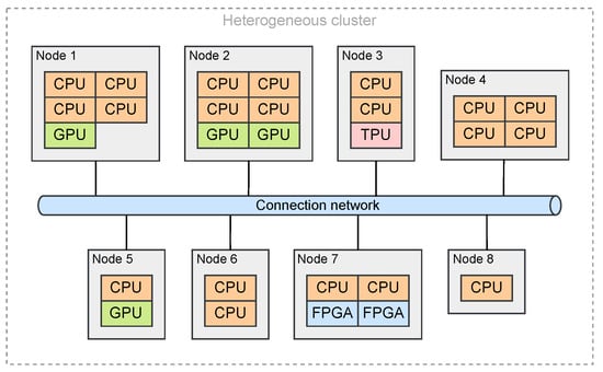
Figure 1.
Simple representation of a heterogeneous cluster. Adapted from [16].
This diversity is especially advantageous for ML workloads, since we can design nodes that are optimised for specific tasks, such as data preprocessing, model training, or inference. By designing nodes to these specific tasks and assigning them accordingly, the overall performance and efficiency of the ML workflow can be significantly enhanced. This approach also helps prevent overloading a single machine, even if it has multiple types of processing devices.
3.2. MLOps
MLOps consists of a combination of tools, processes, and practices that aim to automate and streamline the development, deployment, and maintenance of ML systems in production. At its core, MLOps applies the concepts of Development and Operations (DevOps) that are relevant to the ML field, and creates new practices exclusive to ML systems. The main objective of MLOps is to close the gap between data science teams, who focus on building and training models, and operations teams, who are responsible for ensuring the stability, scalability, and reliability of production systems.
As illustrated in Figure 2, the MLOps workflow consists of a sequence of well-defined stages that covers the full lifecycle of an ML model, from data acquisition to post-deployment monitoring. The workflow begins with data collection, also referred to as data ingestion, where raw data is gathered from various sources, such as relational databases, web APIs, or streaming platforms. After data is collected, it proceeds to the data preprocessing stage, where it is cleaned and transformed to be suitable for ML tasks. Common steps in this stage include handling missing values, normalising numerical features, encoding categorical variables, and identifying or removing outliers.
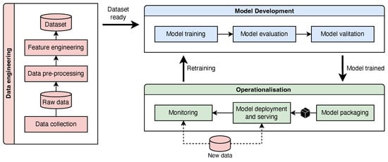
Figure 2.
MLOps workflow. Adapted from [17].
Following preprocessing, the next step is feature engineering. In this phase, relevant features are selected and extracted, new features may be created, and the dimensionality of the dataset is often reduced. The result of these data preparation steps is a refined dataset that is typically split into training, validation, and test sets for use in model development. Once the data is prepared, model training takes place. Here, an ML algorithm is applied to the training dataset to learn underlying patterns and relationships within the data.
After the model has been trained, it is evaluated using the test dataset to assess its performance. This evaluation includes calculating metrics such as accuracy, precision, recall, and F1 score. If the model achieves acceptable performance, it moves on to the validation phase. During validation, the model is compared against baseline models and previous versions to ensure it offers a meaningful improvement. If the validation results are positive, the model is then deployed to a production environment where it is used to make predictions on new, unseen data.
Once deployed, the model is continuously monitored to detect potential issues such as performance degradation, concept drift, or data drift. If such problems are identified, the model may need to be retrained using updated data and then redeployed to maintain performance standards.
To support the automation of the workflow, each stage from data collection to model validation is typically implemented as a modular and reusable component. These components are executed in a specific order, commonly referred to as an ML pipeline. A common approach in MLOps is to containerise each pipeline step using tools like Docker and to manage and orchestrate them with container orchestration systems. Existing MLOps platforms offer built-in tools to facilitate the orchestration and management of these pipelines.
4. Proposed Approach
While existing MLOps platforms offer valuable tools for implementing MLOps principles, they often lack robust support for efficiently executing ML pipelines in heterogeneous environments. Furthermore, as discussed in Section 2, few studies have addressed this issue, and none have proposed a practical solution that can be easily adopted in real-world scenarios.
To address this gap, we propose a modular and flexible placement system for ML pipelines. This system automatically assigns each pipeline task to a suitable machine to minimise the overall execution time and pipeline waiting time. Recognising the diverse nature of ML pipelines and the inherent heterogeneity of modern clusters, the system is also designed to be extensible and adaptable by enabling the integration of custom placement strategies.
Crucially, this system is not intended to replace existing MLOps platforms, which already provide essential and complex features. Instead, its objective is to augment them by offering currently lacking placement and scheduling capabilities.
4.1. Architecture
To enable seamless integration with existing MLOps platforms, the placement system is designed to operate as an independent, decoupled layer. This logical separation ensures broad compatibility, allowing the system to operate without requiring significant changes to the underlying platform.
Regarding the system’s architecture, it is designed to be modular, allowing for flexibility and extensibility. As shown in Figure 3, it comprises five core components: the Pipeline Manager, Node Manager, Data Manager, Model Estimator, and Placement Decision Unit. Each component has a well-defined role and collaborates with the others to achieve the desired placement and scheduling functionality.
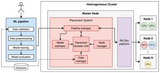
Figure 3.
Proposed solution architecture. The proposed system (red box) acts as an intermediary between the user and the MLOps platform (purple box). It receives an ML pipeline (blue box), which the Pipeline Manager breaks into individual tasks for analysis. Based on the solution components, the Placement Decision Unit determines an appropriate node for each pipeline task, as well as the execution order of the received pipelines. Finally, the Pipeline Manager delegates the pipeline to the MLOps platform, which executes it on the selected nodes.
As shown in Figure 3, the Pipeline Manager acts as the system’s entry point, enabling users to submit their ML pipelines for execution. It decomposes each pipeline into individual tasks and interacts with the Placement Decision Unit to identify the appropriate nodes for execution. Once the placement decisions are made, the Pipeline Manager triggers the execution of the pipelines and monitors their real-time progress.
The Node Manager is responsible for maintaining and retrieving up-to-date information about all nodes in the cluster, including their computational capabilities and current workload status. This information is crucial for informed decision making and is made available to the Placement Decision Unit.
The Data Manager handles the retrieval of input data characteristics for each pipeline, such as the dataset’s size on disk and its expected memory usage during execution. Complementing this, the Model Estimator estimates the computational complexity of models used in pipelines, quantified by the number of operations required for training and evaluation.
Finally, the Placement Decision Unit integrates all information supplied by the other components to determine the most suitable node for each task within a pipeline. In alignment with the objective of minimising pipeline waiting times, this unit not only selects appropriate nodes but also defines the execution order of the pipelines. As explained earlier, to ensure the system’s flexibility and adaptability, these scheduling and placement decisions are determined by a placement strategy, which can be customised to meet specific workloads and cluster characteristics.
Once pipelines are scheduled and their tasks assigned to nodes, the Pipeline Manager interacts with the MLOps platform to trigger their execution. The system itself does not execute the pipelines; instead, it supplies the necessary placement information to the platform, which remains responsible for orchestrating execution on the selected nodes.
As illustrated in Figure 4, the system’s modular architecture and loosely coupled components enable it to scale horizontally by deploying multiple instances of each module. This design promotes a clear separation of concerns, ensuring that no single component becomes a performance bottleneck as the number of pipelines increases. For example, to support a higher rate of pipeline submissions, multiple Pipeline Manager instances can be instantiated, each responsible for managing a subset of pipelines. The unique component that does not scale horizontally is the Placement Decision Unit, as it needs to maintain a global view of the pipelines to make informed placement decisions.
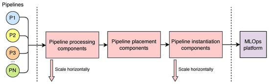
Figure 4.
Proposed solution scalability.
Another key enabler of this scalability is the architectural decision to delegate the execution of ML pipelines to an external MLOps platform. By offloading computationally intensive tasks, the placement system remains focused on the scheduling and placement process. This approach keeps the system lightweight and capable of efficiently processing a large number of placement requests.
While the modular architecture significantly contributes to scalability, actual performance also depends on implementation details. Therefore, Section 5 provides a more detailed discussion of the system’s scalability and robustness.
4.2. Placement Strategy
Although the system is designed to support the integration of custom placement strategies, in this work, we propose a specific strategy to demonstrate its potential and effectiveness. The strategy comprises two sequential phases: (i) pipeline scheduling and (ii) task placement.
In the first phase, the strategy determines the execution order of pipelines with the objective of minimising waiting time. In the second phase, each task within a pipeline is assigned to an appropriate node to reduce the overall pipeline execution time. Both phases are described in detail in the following subsections.
4.2.1. Pipeline Scheduling
In order to reduce waiting times, the system cannot execute the pipelines in the order they are received. For example, if a pipeline with a long execution time is received first, it may block the execution of other pipelines that could be completed quickly.
To overcome this issue, first, the system accumulates multiples pipelines during a certain period of time, defined as a time window. Once the window closes, the strategy sorts the pipelines based on their estimated execution length following the Shortest Job First (SJF) scheduling algorithm.
In the context of ML, accurately predicting the execution time of a pipeline is challenging due to variability in ML algorithms and the heavy dependence on hyperparameters, input data, and available hardware. To address this challenge, the strategy assumes the length of a pipeline as the sum of the number of operations required for each task in the pipeline. This approach is based on the assumption that the execution time of a task is proportional to the number of operations it performs.
The calculation of the number of operations performed by training and evaluation tasks is derived from model parameters, data characteristics, and, most importantly, the theoretical computational complexity of the ML algorithms used. Although current ML libraries are highly optimised, and the actual number of operations may be inferior to the theoretical one, obtaining the total number of operations from the theoretical complexity of the algorithms is a reasonable approximation for effective scheduling.
4.2.2. Pipeline Task Placement
Once the execution order is established, the second phase involves assigning each task to a suitable node within the heterogeneous cluster. Since the task placement problem is known to be NP-hard [18], the proposed strategy does not aim to compute an optimal solution, as this would be computationally expensive and unsuitable for real-time placements. Instead, a heuristic-based approach is employed to find a sufficiently good solution within a short time frame.
To simplify the strategy, the approach assumes three possible types of tasks in a pipeline: data preprocessing, model training, and model evaluation. Data preprocessing tasks include typical operations such as data validation, cleaning, transformation, and dataset splitting. Model training tasks involve the training of ML models on the training dataset, while model evaluation tasks assess the performance of the trained models on the test dataset.
While the majority of preprocessing tasks are usually lightweight and do not require significant compute resources when compared to training tasks, their success is highly dependent on the capacity of a node to handle the input data. If the selected node does not have enough memory to load and process the data, all the subsequent tasks in the pipeline will fail. To mitigate this risk, the proposed strategy selects a node for data preprocessing tasks based on the size of the input data and the available memory on each node. Specifically, it selects a node whose available memory exceeds the size of the input data plus an additional margin to account for overhead.
In the case where multiple nodes meet the memory requirements for a preprocessing task, the strategy selects the one with the lowest current load. The current load of a node is defined as the number of tasks assigned to that node at the time of placement. This approach helps to balance the workload across the cluster and avoid overloading any single node.
For model training and evaluation tasks, the strategy assumes that the heterogeneous nodes in the cluster are organised into groups that reflect their processing capabilities. Using these groups, the strategy selects the appropriate node for each task using a model-to-group mapping, which is defined as a set of rules that specify which models can be executed on which groups of nodes. Each rule consists of three components: the model type, the task type (training or evaluation), and the group of nodes that can execute the model.
During task placement, if multiple nodes satisfy the model-to-group mapping criteria, the strategy selects the node with the lowest current load. If none of these nodes have sufficient memory to accommodate the input data, the strategy defaults to a fallback node. The fallback node is defined as the node within the cluster that possesses the lowest load while also having adequate memory to handle the input data.
A common behaviour of popular cluster orchestration tools, such as Kubernetes, is to start executing a workload as soon as it is submitted. In the context of ML pipelines, if multiple pipelines are submitted concurrently, they may start executing simultaneously, potentially resulting in multiple tasks being assigned to the same node. This can lead to resource contention and degraded performance, particularly for training tasks, which tend to be the most resource-intensive.
To ensure that different pipelines do not compete for the same resources, the system forces each node to execute a single task at a time. However, a limitation of this approach is that some nodes assigned to a pipeline may remain idle while waiting for a task on another node to complete. To mitigate this problem, the placement strategy attempts to minimise the number of distinct nodes assigned to the tasks within a pipeline, as long as the nodes have the required resources available and fulfil the model-to-group mapping criteria. This allows multiple pipelines to run simultaneously without competing for the same resources.
To summarise the task placement process, Algorithm 1 outlines the main steps involved. In a scenario where two pipelines are submitted, each comprising a preprocessing task followed by a training task, the proposed strategy begins by sorting the pipelines according to their estimated length, following the SJF algorithm. The strategy then iteratively processes each pipeline and its associated tasks to determine appropriate node assignments. For preprocessing tasks, it filters available nodes based on memory capacity and selects the least-loaded node capable of handling the input data. For training tasks, the strategy retrieves candidate nodes according to the model-to-group mapping and filters them based on memory capacity. If any of these nodes were already assigned to the pipeline being processed, it selects the least-loaded node among them; otherwise, it chooses the least-loaded node from the full candidate set. If no suitable nodes are found, a fallback node is selected. Finally, the strategy updates the task-to-node assignment map and increments the load of the selected node to reflect the new assignment.
| Algorithm 1 Pipeline task placement base algorithm. | |
| Input: P List of sorted pipelines using the SJF algorithm | |
| Input: N List of cluster nodes | |
| Input: M Model-to-group mapping (model and task type to node groups) | |
| Output: A Assignment map of tasks to nodes for each pipeline | |
| 1: | |
| 2: | ▹ Load of each node (number of tasks assigned) |
| 3: | ▹ Current pipeline being processed |
| 4: | ▹ Current task being processed |
| 5: | ▹ Candidate nodes for task t |
| 6: | ▹ Node groups from model-to-group mapping |
| 7: | ▹ Nodes already assigned to pipeline p |
| 8: | ▹ Nodes already assigned to pipeline p that meet the mapping |
| 9: | ▹ Node selected for task t |
| 10: | |
| 11: for each p in P do | |
| 12: | |
| 13: for each t in p do | |
| 14: if is preprocessing then | |
| 15: ← filter_by_sufficient_memory(N, ) | |
| 16: ← least_loaded_node(, L) | |
| 17: else | |
| 18: ← get_groups_from_mapping(M, , ) | |
| 19: ← get_nodes_from_groups(N, ) | |
| 20: ← filter_by_sufficient_memory(, ) | |
| 21: ← nodes_assigned_to_pipeline(p) | |
| 22: ← intersection(, ) | |
| 23: if is not empty then | |
| 24: ← least_loaded_node(, L) | |
| 25: else | |
| 26: ← least_loaded_node(, L) | |
| 27: end if | |
| 28: end if | |
| 29: if is null then | |
| 30: ← get_fallback_node(N, , ) | |
| 31: end if | |
| 32: node | ▹ Assign task t from pipeline p to node |
| 33: | ▹ Increment node load |
| 34: end for | |
| 35: end for | |
| 36: | |
| 37: return A | |
As stated in Section 4.1, the placement component was not designed for horizontal scalability. This could become a bottleneck for the execution of the proposed approach. However, there are two critical operations within the proposed approach: sorting the pipelines by their estimated length and employing the heuristic (described in Algorithm 1). Sorting the pipelines has an algorithmic complexity of . Regarding the heuristic, it contains a main loop that iterates through all pipelines, followed by a nested loop that iterates through all stages of each pipeline. Other operations are nearly constant time, as they primarily involve quick look-ups to filter nodes based on various criteria. Therefore, the algorithmic complexity can be approximated by the number of pipelines waiting to be placed (disregarding the pipeline stages, which are mostly fixed at four or five). This leads to a linear complexity of . Although the heuristic could potentially become a bottleneck, the low algorithmic complexity of these critical operations confirms the low overhead of the proposed method.
5. Implementation
Building upon the conceptual framework, we implemented the proposed placement system to validate its practical feasibility. This section provides a detailed explanation of the implementation, covering the definition and submission of ML pipelines, the estimation of pipeline execution lengths, and the allocation of tasks across available nodes. The source code for this implementation is publicly available at: https://github.com/pedro535/ml-pipeline-placement (accessed on 15 May 2024).
5.1. Pipeline Definition and Submission
As discussed in Section 3, an ML pipeline consists of a sequence of tasks executed in a defined order. Each pipeline can be represented as a Directed Acyclic Graph (DAG), where nodes correspond to individual tasks and edges represent dependencies between them.
To promote modularity and task reuse, the implemented system requires each task to be encapsulated within a standalone Python file. These files include not only the core task logic but also any necessary libraries and dependencies. To further support modularity, each task must be implemented as a Python 3 function, allowing it to be easily imported and reused across different pipelines.
Once individual tasks are implemented, they are grouped to form a pipeline. Similar to task definition, the pipeline itself is also defined in a separate Python file where the previously defined tasks are imported as standard Python modules. To simplify the pipeline definition process, we developed a Python package, which provides intuitive abstractions for defining pipelines. With this package, it is possible to define input and output data paths, task-specific parameters, and also the execution order of tasks, thereby constructing a DAG that accurately reflects task dependencies.
In order to provide relevant information about the pipeline and the input data used to the system, along with the task files, the user must also provide a pipeline metadata file. This consists of a JSON file that contains information about the input data, such as the number of samples and features, as well as the data types of each feature. The metadata file is essential for estimating the memory requirements of the pipeline tasks, which is crucial for the task placement process.
The implemented package also provides a submission utility function for pipeline submission. This function sends all pipeline task files, the pipeline definition file, and the metadata file to the placement system, which exposes an Representational State Transfer (REST) API that listens for incoming submissions. Following this approach, submitting a pipeline is straightforward, since we only need to execute the pipeline definition script like any Python script. Figure 5 illustrates the definition and submission process of a pipeline.
Figure 5.
Overview of the pipeline definition and submission process. Each task is implemented as a Python function in a separate file. The pipeline definition file imports these task functions, specifies their parameters, and defines their execution order, forming a DAG. Executing the pipeline script triggers the submission process, sending the pipeline to the placement system.
5.2. Pipeline Scheduling
As previously noted, to schedule the received pipelines, the proposed placement strategy employs the SJF scheduling policy, where the length of a pipeline is defined as the total number of operations across all tasks within the pipeline.
For tasks involving model training and evaluation, the number of operations is estimated based on the model type, model-specific parameters, the size of the training or test dataset, and the worst-case time complexity of the model. In the current implementation, the system includes five different estimators corresponding to the following model types: Logistic Regression (LR), Decision Tree (DT), Random Forest (RF), Support Vector Machine (SVM), and Neural Networks (NNs).
Although the literature provides slightly inconsistent definitions of the worst-case time complexity for each model type, we have chosen to adopt the definitions that are most widely accepted. Summarised in Table 2, each time complexity is expressed as a function of the number of training samples n, the number of features m, and the model-specific parameters.
Table 2.
Worst-case time complexity for traditional ML algorithms.
Unlike traditional ML models, the time complexity of NNs depends heavily on architectural factors, such as the number and type of layers. Consequently, it is not possible to derive a universal expression for estimating computational complexity. To address this, we estimate the number of Floating Point Operations (FLOPs) required for training and inference based on the network architecture’s specific characteristics.
The number of operations O required to train a NN can be estimated using the following expression:
where and represent the number of operations performed during a single forward and backward pass, respectively. The total number of passes over the training data, , can be computed as the product of the number of epochs and the number of training examples.
During the backward pass, each layer must compute the gradient with respect to its weights as well as the error gradient with respect to its inputs, to propagate the error backward. Each computation requires a number of operations roughly equivalent to those performed during the forward pass. Consequently, several studies [22,23,24] have found the backward-to-forward FLOP ratio to be approximately stable, with a value of 2:1 being a reasonable approximation [25,26].
Letting R denote the backward-to-forward FLOP ratio, the total number of operations can, thus, be approximated as:
Replacing the ratio R with 2, we can simplify the expression to:
In terms of model inference, the process is much simpler, since it only requires a single forward pass through the network. Therefore, the number of operations required for inference can be expressed as:
where is the number of samples in the test set used for model evaluation.
Finally, to calculate the number of operations for a single forward pass we sum the FLOPs of each layer in the network. Table 3 summarises the expressions used to obtain the FLOPs of fully connected and convolutional layers [27]. In this estimation, the operations of other layer types (e.g., pooling, activation functions, etc.) are not included, as their computational cost is typically negligible compared to that of fully connected and convolutional layers [28].
Table 3.
Expressions to calculate FLOPs for fully connected and convolutional layers.
5.3. Pipeline Task Placement
As outlined in Section 4, the criteria for placing data preprocessing tasks differ from those for model training and evaluation. Data preprocessing tasks are assigned to the least loaded nodes that possess sufficient memory to accommodate the input data, while model training and evaluation tasks are placed according to model-to-group mapping rules.
To estimate the memory required for data preprocessing tasks, the implemented strategy starts by calculating the number of bytes occupied by a single sample in the input dataset. For tabular datasets, this estimation is based on the data types of each feature and the number of bytes required to store each data type. For image datasets, the estimate is derived from the image dimensions, the number of channels, and the data type of the image pixels. The memory usage per sample is then multiplied by the total number of samples to compute the overall memory required for the dataset. To perform this estimation, the involved parameters must be provided by the user in the pipeline metadata file, which is submitted alongside the pipeline.
For training and evaluation tasks, the model-to-group mapping rules are specified in a JSON file, which defines each model type alongside the corresponding node groups on which it should be executed. As previously mentioned, these rules are not universal and should be adapted to the specific characteristics of the cluster and the workloads it is expected to handle.
For this study, the mapping rules were primarily obtained by dividing the complexity of the ML algorithms in three categories that reflect their training complexity: low, medium, and high. The low category includes the algorithms whose training complexity goes from to . The medium category includes algorithms with training complexity greater than and up to . Finally, the high category includes algorithms with training complexity greater than .
Based on the categorisation of the algorithms and the node groups considered for this study (detailed in Section 6), the model-to-group mapping was defined as follows: the low algorithms were assigned to the low and medium groups, the medium algorithms were assigned to the medium and high-CPU groups, and the high algorithms were assigned to the high-CPU and high-GPU groups. For evaluation tasks, which are less computationally intensive than training tasks, each algorithm was mapped to the next lower node group or groups, accordingly.
The mapping rules resulted from this categorisation are summarised in Table 4.
Table 4.
Node groups selected for each model type.
In heterogeneous clusters that include GPU nodes, training NNs is typically significantly faster on GPUs than on CPUs. Consequently, strictly following the least-loaded node policy for such tasks may not yield optimal performance. To address this, when multiple pipelines that benefit from GPU acceleration are submitted, the implemented strategy prioritises queuing the training tasks on GPU nodes, rather than assigning them to available CPU nodes.
To prevent excessive queuing, which could delay pipeline execution or overload the GPU nodes, the system allows for the specification of a maximum number of tasks that may be queued for execution on GPU nodes. Once this threshold is reached, any additional tasks are assigned according to the least-loaded node policy, regardless of whether they benefit from GPU acceleration. This strategy balances the advantages of GPU acceleration with the need to maintain efficient resource utilisation and prevent bottlenecks in pipeline execution.
While this approach is expected to improve execution and waiting times, it may introduce trade-offs in terms of energy consumption. GPUs typically consume significantly more energy than traditional CPUs, particularly under high computational loads. As a result, prioritising GPU usage for accelerated tasks may lead to increased overall energy consumption in the cluster. Nevertheless, the primary focus of this work was to optimise pipeline execution and waiting times, and the energy implications of this strategy were not a primary concern.
5.4. Pipeline Execution
As outlined in Section 4, once the received pipelines have been scheduled and assigned to cluster nodes, the system initiates their execution using an MLOps platform. In this implementation, the placement system leverages Kubeflow, which is a Kubernetes-native MLOps platform that provides essential containerisation and orchestration capabilities for ML pipelines. The system interacts with Kubeflow via its API, explicitly specifying the nodes on which each task should be executed.
The pipelines are executed in the order determined by the scheduling phase, starting with the least complex and progressing to the most complex. The system only triggers the execution of a pipeline once all the required nodes are available. If at least one of the required nodes is unavailable, the pipeline is added to a waiting queue.
To monitor the progress of running pipelines and detect when nodes become available, the system periodically queries the Kubeflow API. This API not only enables the triggering of pipeline execution but also provides real-time status updates for each task. These updates allow the system to track task progress and identify when execution is complete.
5.5. System Scalability and Robustness
As outlined in the previous section, the placement system consists of multiple loosely coupled components, each with clearly defined responsibilities. This modular and flexible architecture enables high scalability, as individual components can be scaled independently based on workload demands.
Beyond its architectural scalability, the implemented system benefits from the capabilities of the underlying MLOps platform, Kubeflow. Built on top of Kubernetes, Kubeflow inherits Kubernetes’ ability to scale horizontally. As the number of pipelines increases, additional nodes can be added to the cluster to accommodate the increased workload, allowing the system to handle larger-scale deployments effectively.
Regarding robustness, the system is designed to adapt to the dynamic nature of heterogeneous clusters, where nodes may be added, removed, or become temporarily unavailable. Before each placement operation, the system queries the Kubernetes API to identify currently available nodes and retrieve their specifications. If a node is unavailable due to failure or connectivity issues, it is excluded from the placement process, ensuring that tasks are only scheduled on operational nodes. This enhances the system’s overall fault tolerance and reliability.
If a node fails during pipeline execution, the implemented system is able to detect this failure through both the Kubernetes API and the Kubeflow API. However, as this implementation focuses primarily on pipeline placement and scheduling, automatic rescheduling mechanisms for failed tasks were not implemented. Instead, the system relies on the built-in fault-tolerance features of the underlying MLOps platform to manage task failures and retries.
In summary, the modular architecture and the clear separation between the placement system and the underlying MLOps platform contribute significantly to the scalability and robustness of the proposed solution. Furthermore, the system’s awareness of the cluster’s current state and the status of ongoing tasks enables it to dynamically adapt to environmental changes, ensuring reliable and efficient pipeline execution.
6. Evaluation
To evaluate the performance of the proposed solution, we conducted a series of experiments in which multiple ML pipelines were submitted under two different scenarios. To assess the impact of our approach, we also implemented several baseline strategies for comparison. The following subsections detail the experimental setup, the baseline methods, the ML pipelines used, and the evaluation scenarios. Finally, we present and discuss the results obtained from these experiments.
6.1. Experimental Setup
The experiments were conducted using a Kubernetes cluster comprising 11 nodes: 10 worker nodes and 1 master node. As their name implies, the worker nodes are responsible for executing the ML tasks, while the master node is responsible for executing the implemented placement system and the MLOps platform.
In terms of heterogeneity, as already introduced in Section 5, three different types of worker nodes were considered: low, medium, and high performance nodes. As presented in Table 5, each node type differs in terms of the amount of Random Access Memory (RAM) available, the number of CPU cores, and CPU architecture. To include accelerated hardware in the evaluation, an additional high performance node was added, which is equipped with a GPU.
Table 5.
Worker nodes considered in the experiment.
6.2. Baselines
To evaluate whether the proposed solution effectively optimises the execution of ML pipelines, it is necessary to compare its performance with alternative methods. While an intuitive choice would be to use the approaches discussed in Section 2, these are primarily conceptual or exploratory in nature and lack practical implementations. As a result, a direct performance comparison with existing literature is not feasible.
To overcome this limitation, three alternative placement strategies were implemented as baselines. Similar to the proposed approach, these baselines incorporate both scheduling and placement phases.
The first baseline, designed to represent a naïve approach, implements an entirely random placement strategy. In this strategy, both the execution order of the pipelines and the assignment of tasks to nodes are determined randomly. While this approach is expected to yield poor performance, it serves as a valuable point of reference, helping to quantify how much the proposed solution improves over a placement strategy with no informed decision making.
The second baseline strategy adopts an First-Come First-Served (FCFS) approach for scheduling. In this strategy, pipelines are executed in the exact order in which they are submitted rather than randomly selected. However, the placement of tasks within the pipelines remains random.
In the previous baseline strategies, there is the risk that a task may be assigned to a node without sufficient memory to accommodate its input data. To prevent execution failures, if the initially selected node lacks adequate memory, another node is randomly selected until a suitable one is found.
Finally, the third baseline also adopts the FCFS approach for scheduling. However, unlike the previous strategies, it employs the Round Robin (RR) method for placement. In this approach, tasks are cyclically assigned to nodes, distributing the workload evenly across the cluster. As with the other baselines, if a selected node does not have enough available memory for a given task, the next node in the sequence is selected, continuing this cycle until an appropriate node is found.
Since this work is situated within the context of MLOps, it is also relevant to compare the proposed solution with leading open-source MLOps orchestration tools, such as Apache Airflow, Argo Workflows, and MLflow. A common characteristic of these tools is their reliance on Kubernetes and its default scheduler for pipeline scheduling and placement. For this reason, the default Kubernetes scheduler was also included in our evaluation. However, since this method differs from the proposed solution in the sense that it does not implement a waiting queue for pipelines (executing them immediately upon submission), it was not considered a baseline in the strict sense, but rather a point of reference for comparison.
6.3. ML Pipelines
The ML pipelines considered in the evaluation consist of three sequential tasks: data preprocessing, model training, and model evaluation. The data preprocessing step involved loading the dataset, performing light transformations (e.g., removing duplicates, normalising the data), and splitting the data into training and test sets. The model training step focused on training the model using the training set, while the model evaluation step assessed the trained model on the test set.
A total of 18 distinct ML pipelines were created, comprising 3 pipelines for each of the following models: LR, DT, RF, SVM, Deep Neural Network (DNN), and Convolutional Neural Network (CNN).
In terms of datasets, total of nine distinct datasets were utilised, varying in size and characteristics. Of these, five were tabular datasets, and the remaining four were image datasets. All the datasets are publicly available, designed for classification problems, and widely used by the ML community for benchmarking ML models.
A summary of the developed pipelines, including the datasets and their associated ML models, is presented in Table 6.
Table 6.
Pipelines used for evaluation.
6.4. Evaluation Scenarios
The first scenario investigated the system’s ability to accelerate the execution of ML pipelines under concurrent submission. For this evaluation, two pipelines were submitted for each model type within the same time window. The system’s performance was measured based on total execution time and average pipeline waiting time. Total execution time refers to the interval between the start of the first pipeline’s execution and the completion of the last. Average waiting time represents the mean duration each pipeline spent in the waiting queue from submission until the start of execution.
To ensure a fair comparison, the order in which the pipelines were submitted was randomised. Additionally, for the Kubernetes scheduler and baseline strategies involving randomness, each experiment was repeated five times, and the average execution time and waiting time were calculated.
The second scenario aimed to assess the system’s capability to promptly dispatch pipelines. For this evaluation, the 18 pipelines were organised into 3 groups of 6. Each group was submitted simultaneously, with successive groups introduced at four-minute intervals. The system performance was measured by tracking the changes in the number of running and waiting pipelines over time as new submissions were introduced. As in the first scenario, the order of pipeline submissions within each group was randomised.
Table 7 summarises the pipelines used in each evaluation scenario, along with the order in which they were submitted.
Table 7.
Pipelines executed in each evaluation scenario.
In both scenarios, the time window was set to 15 s, which was sufficient for the pipelines considered in this evaluation. As the cluster includes a node equipped with a GPU, the maximum number of tasks waiting for execution on GPU was set to three. When this limit is reached, the placement system defaults to assigning tasks based on the least-loaded node policy, explained in Section 5.
6.5. Results
This section presents the obtained results for the evaluation scenarios described above. For each scenario, we provide a detailed analysis of the proposed strategy in comparison with the baseline approaches.
6.5.1. First Scenario
Regarding the first scenario, Figure 6 and Figure 7 show the total execution time and the average waiting time for each strategy, respectively. The Kubernetes scheduler is excluded from Figure 7, as the pipelines are executed immediately upon submission.
Figure 6.
Total execution time for each strategy. Error bars are shown only for strategies involving randomness and for the Kubernetes scheduler.
Figure 7.
Average waiting time for each strategy. Error bars are shown only for strategies involving randomness.
As shown in Figure 6, the proposed strategy achieves the best performance among all evaluated approaches, with a total execution time of 285 s. The next best result is from the Kubernetes scheduler, with a total execution time of 404.2 s. In contrast, the baseline strategies exhibited significantly longer execution times, ranging from 859 to 890.8 s. Despite the differences in their internal scheduling and placement mechanisms, the baseline strategies performed similarly.
To better illustrate the performance improvements, Table 8 presents the reduction in total execution time both as a percentage and as a speed-up factor compared to the baseline strategies and the Kubernetes scheduler.
Table 8.
Reduction in total execution time achieved by the proposed strategy.
According to this table, the proposed strategy was approximately three times faster than the baseline approaches and 1.42 times faster than the Kubernetes scheduler. This translates to a reduction in total execution time between 66.82 percent and 68.01 percent compared to the baselines, and a reduction of 29.49 percent relative to the Kubernetes scheduler.
A similar pattern appears when examining the average waiting time. As shown in Figure 7, the proposed strategy resulted in the lowest average waiting time, with a value of 54.3 s. In comparison, the baseline strategies exhibited substantially higher average waiting times, ranging from 245.5 to 281.9 s. As detailed in Table 9, this represents a reduction in average waiting time between 77.88 percent and 80.74 percent, which corresponds to a speed-up factor between 4.52 and 5.19.
Table 9.
Reduction in average waiting time achieved by the proposed strategy.
These performance gains are due to the fact that the proposed strategy selects nodes based on model characteristics, considers the current load on each node, and tries to reuse the same nodes for a pipeline. This promotes higher parallelism and efficient execution.
As an alternative perspective, Figure 8 and Figure 9 present the execution times and waiting times for each individual pipeline across all evaluated strategies, respectively. The pipelines are shown in the order in which they were submitted, from left to right. An important aspect to note in Figure 8 is that the sum of the execution times for each pipeline should not coincide with the total execution time presented in Figure 6, as multiple pipelines run concurrently. Instead, this figure is intended to provide a more detailed view of how the strategies influenced the performance of each individual pipeline.
Figure 8.
Execution time of each pipeline for each strategy.
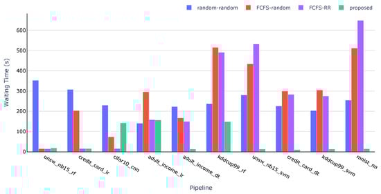
Figure 9.
Waiting time of each pipeline for each strategy.
As shown in Figure 8, the execution times for pipelines that do not involve NNs are similar across all strategies. While the differences are not significant (maximum of 21 s), the Kubernetes scheduler occasionally achieves slightly better performance. This is primarily because all the tasks were placed on medium and high-performance nodes, leaving all low-performance nodes unused. However, this behaviour may lead to performance degradation for more complex pipelines, as the scheduler often concentrates workloads on the most capable nodes, resulting in resource contention and longer execution times.
A similar pattern is observed in the baseline strategies involving random placement. As can be seen in Figure 8, the execution times for non-NN pipelines are again similar to those of the Kubernetes scheduler. This is largely due to the higher probability (70%) of randomly selecting medium- or high-performance nodes, which leads to task distributions comparable to those of the Kubernetes scheduler. Consequently, the Random-Random and FCFS-Random strategies exhibit similar performance in this context.
For pipelines involving NNs, the proposed strategy clearly outperforms all others by successfully allocating these pipelines to high-performance nodes, including the one equipped with a GPU. In contrast, the other strategies lack awareness of hardware acceleration, and therefore, they fail to assign NN-based pipelines to an appropriate node.
Regarding pipeline waiting time, as illustrated in Figure 9, the proposed strategy consistently achieves lower waiting times compared to the baselines. The obtained values indicate that it was able to execute seven pipelines in parallel, while the remaining three had to wait for nodes to become available.
Another important observation is that the proposed strategy was able to prioritise the execution of less complex pipelines before the more complex ones. The only exception to this was the “adult income” pipeline using an LR model, which experienced a delay due to at least one node already being occupied by other pipelines.
The importance of selecting appropriate nodes and adopting a scheduling technique becomes evident when comparing the proposed strategy with the FCFS-RR strategy. In the latter, the most computationally demanding pipeline (“cifar10_cnn”) was assigned to a medium-performance node, resulting in a cascading delay that increased the waiting times for all subsequent pipelines.
6.5.2. Second Scenario
Regarding the second scenario, where three groups of six pipelines were submitted at four-minute intervals, the results are presented in Figure 10, Figure 11, Figure 12 and Figure 13. These figures illustrate the evolution of the number of running and waiting pipelines over time. For the same reason as in the first scenario, the Kubernetes scheduler is excluded from these experiments since it does not have the concept of waiting pipelines.
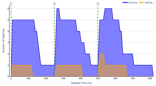
Figure 10.
Running and waiting pipelines over time for the proposed strategy.
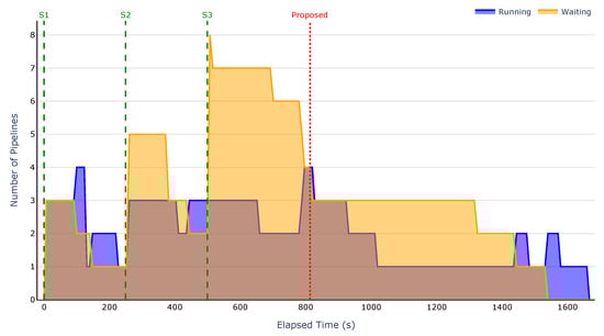
Figure 11.
Running and waiting pipelines over time for the Random-Random strategy.
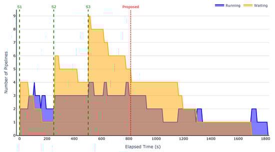
Figure 12.
Running and waiting pipelines over time for the FCFS-Random strategy.
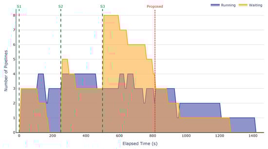
Figure 13.
Running and waiting pipelines over time for the FCFS-RR strategy.
The results clearly demonstrate that the proposed strategy enables prompt dispatching of pipelines. As shown in Figure 10, there are no waiting pipelines at submission time, and only one pipeline is running. In contrast, the baseline strategies fail to appropriately map pipelines to nodes and do not prioritise simpler pipelines. This results in an early accumulation of waiting pipelines, leading to an overall increase in execution time.
As in the previous scenario, the accumulation of waiting pipelines results in a cascading effect, where the number of pending pipelines increases with each submission. This behaviour is particularly evident in Figure 12, where the number of waiting pipelines starts at four, rises to six after the second submission, and reaches nine after the third, negatively impacting the overall execution time.
Across all scenarios, our strategy executed up to six pipelines in parallel, while the baselines managed only four. This improvement comes from two key factors: the strategy’s ability to reuse nodes for different tasks within the same pipeline, and its prioritisation of less complex pipelines, which prevents early bottlenecks.
As detailed in Table 7, for this scenario, each submitted group comprised two pipelines involving NNs. Since the proposed strategy prioritises waiting for a GPU node to become available rather than assigning training tasks to CPU nodes, after the first submission, the training tasks from both pipelines were assigned to the GPU node. Since each node can execute only one task at a time, the more complex pipeline was placed on the waiting list. That is why, in Figure 10, the number of pipelines on the waiting list increased to one. This behaviour was repeated with the second group of pipelines.
After the third submission, since the GPU node was still occupied by a training task from the second group, both pipelines involving NNs were added to the waiting list. This happened because the training tasks from both pipelines were assigned to the GPU node, as the limit defined for waiting tasks on GPU nodes was not reached.
If the least-loaded node policy had been used for all ML algorithms, after the third submission, the proposed strategy would have distributed both training tasks across high-performance nodes without GPU, as they were available during the placement. This alternative assignment would have resulted in longer execution times for both pipelines, compromising the overall responsiveness of the system.
Since this scenario involved executing all the developed pipelines, it is also relevant to analyse the correlation between the execution time of the pipelines and the size of the datasets used. Table 10 presents the Spearman correlation coefficients between the execution time of the pipelines and the size of the datasets for each strategy. We omitted the correlation of the Random-Random approach, as it is entirely related to chance (specifically, the seed value used) and does not provide any useful information. For tabular datasets, the size corresponds to the multiplication of the number of samples by the number of features. For image datasets, the size is calculated as the product of the number of samples and the size of each image ().
Table 10.
Correlation between pipeline execution time and dataset size.
As we can see, our approach presents a higher level of correlation among the execution time and the dataset size, validating the results that our approach makes better use of the heterogeneous resources and reduces the overall execution time of the various pipelines
In summary, the results from both scenarios demonstrated that the proposed solution effectively optimises the execution of ML pipelines in environments with heterogeneous resources. The performance gains can be attributed to three key factors: the model-to-group mapping, which enabled efficient task assignment based on model characteristics; the strategy’s focus on maximising the number of concurrently running pipelines; and the prioritisation of smaller pipelines to prevent delays for subsequent ones.
However, for pipelines whose training tasks do not require GPU acceleration, the strategy performed slightly worse than the Kubernetes scheduler and the baselines involving random placement. This was due to the assignment of such tasks to low- and medium-performance nodes, whereas the other strategies favoured higher-performance nodes. Nevertheless, this trade-off was necessary to ensure that all nodes in the cluster were utilised.
7. Conclusions
This paper proposes a modular and flexible placement system aimed at optimising the execution of ML pipelines in heterogeneous clusters, particularly within the context of MLOps. While the system is designed to support custom placement strategies, a two-phase strategy is presented. In the first phase, pipelines are scheduled following the SJF algorithm based on the estimated number of operations performed by training and evaluation tasks. In the second phase, each task is assigned to an appropriate node using a heuristic-based placement method. This heuristic employs a model-to-group mapping, defined as a set of rules indicating which models can be executed on which groups of nodes.
After scheduling and node assignment, the system delegates pipeline execution to an existing MLOps platform, which manages the orchestration and execution of tasks. This logical separation between placement and execution enhances flexibility and modularity, thereby improving the system’s scalability and adaptability across diverse scenarios.
To evaluate the proposed system, two experimental scenarios were considered. The first focused on assessing its ability to accelerate pipeline execution under concurrent submissions, while the second examined its responsiveness in dispatching pipelines. For comparative analysis, three baseline strategies were implemented: Random-Random, FCFS-Random, and FCFS-RR. Additionally, the default Kubernetes scheduler was used as a reference point.
Experimental results indicate that the proposed system significantly outperforms the baseline strategies in terms of both total execution time and average waiting time. In the first scenario, the system achieved a reduction in total execution time of up to 68% compared to the baselines, and a 29.5% reduction relative to the default Kubernetes scheduler. Furthermore, it reduced the average pipeline waiting time by as much as 80.7% compared to the baselines. The average waiting time was not measured for the Kubernetes scheduler, as it initiates execution immediately upon submission.
In the second scenario, the system demonstrated effective pipeline dispatching. Batches of six pipelines were submitted at four-minute intervals, and the system consistently cleared the waiting queue before the arrival of the next batch. In contrast, the baseline strategies were unable to do so, resulting in a cascading effect that increased both execution and waiting times.
While the proposed solution demonstrates significant improvements in executing ML pipelines, it is not without limitations. First, the heuristic-based placement strategy relies on predefined rules, which may not adapt effectively to dynamic changes in the cluster or workload. Second, determining the number of operations based on theoretical computational complexity may not accurately reflect the actual execution time of pipelines, particularly for algorithms that benefit from hardware acceleration. This discrepancy can result in suboptimal scheduling decisions. Third, the current evaluation does not sufficiently explore complex or extreme scenarios, limiting the understanding of the system’s robustness and performance under more demanding conditions.
Given these limitations, several avenues for future enhancement emerge. A key direction for future work is the development of a more adaptive task placement strategy. Making the strategy responsive to changing workloads and cluster conditions could significantly enhance the system’s performance. This may involve leveraging ML or RL techniques to enable the system to learn from historical data and real-time metrics. In the case of RL, the placement strategy could treat the current state of the cluster and the characteristics of incoming pipelines as environmental states, and use a reward system based on the performance of placement decisions, such as execution time and resource utilisation. This approach would improve the system’s adaptability without requiring manual adjustments to the placement heuristic.
Another promising area for improvement is the prediction of pipeline execution times. Rather than using the number of operations to represent a pipeline’s length, incorporating lightweight profiling techniques or leveraging historical execution data from similar pipelines could yield more accurate performance estimates. These improvements would enable more informed scheduling decisions and further enhance overall system efficiency.
Future work should focus on evaluating the system across a wider range of realistic and heterogeneous scenarios. Although the current evaluation provides valuable insights, validating the system with a broader spectrum of ML pipelines and cluster configurations is essential to fully assess its adaptability and robustness. Additionally, it would be beneficial to examine the system’s performance under extreme or highly variable conditions.
Finally, although improvements in execution and waiting times often correlate with more efficient resource utilisation, conducting a dedicated analysis of resource utilisation metrics is essential. Future evaluations should, therefore, include explicit measurements of key resource metrics, such as CPU and memory usage, to provide a more comprehensive understanding of the system’s overall performance.
Author Contributions
Conception, methodology, and software: P.R.; Validation, formal analysis, and supervision: J.C., M.A. and R.L.A.; Writing—original draft preparation: P.R. and J.C.; writing—review and editing: M.A. and R.L.A. All authors have read and agreed to the published version of the manuscript.
Funding
This work was supported by FCT—Fundação para a Ciência e Tecnologia, I.P. by project reference UIDB/50008, and DOI identifier 10.54499/UIDB/50008. This work was partially funded by the PRR—Plano de Recuperação e Resiliência and by the NextGenerationEU funds at University of Aveiro, through the scope of the Agenda for Business Innovation “NEXUS: Pacto de Inovação - Transição Verde e Digital para Transportes, Logística e Mobilidade” (Project nº 53 with the application C645112083-00000059).
Data Availability Statement
The data used in this study are publicly available from the following sources: Adult Income: https://archive.ics.uci.edu/dataset/2/adult (accessed on 21 June 2025); Wine Quality: https://archive.ics.uci.edu/dataset/186/wine+quality (accessed on 21 June 2025); Credit Card: https://archive.ics.uci.edu/dataset/350/default+of+credit+card+clients (accessed on 21 June 2025); kddcup99: https://kdd.ics.uci.edu/databases/kddcup99/kddcup99.html (accessed on 21 June 2025); UNSW-NB15: https://research.unsw.edu.au/projects/unsw-nb15-dataset (accessed on 21 June 2025); MNIST: http://yann.lecun.com/exdb/mnist/ (accessed on 21 June 2025); Fashion MNIST: https://github.com/zalandoresearch/fashion-mnist (accessed on 21 June 2025); CIFAR-10: https://www.cs.toronto.edu/~kriz/cifar.html (accessed on 21 June 2025); Citrus fruits and leaves: https://data.mendeley.com/datasets/3f83gxmv57/2 (accessed on 21 June 2025); All datasets are cited appropriately in the manuscript.
Conflicts of Interest
The authors declare no conflicts of interest.
References
- Esteva, A.; Kuprel, B.; Novoa, R.A.; Ko, J.; Swetter, S.M.; Blau, H.M.; Thrun, S. Dermatologist-level classification of skin cancer with deep neural networks. Nature 2017, 542, 115–118. [Google Scholar] [CrossRef] [PubMed]
- Bojarski, M.; Del Testa, D.; Dworakowski, D.; Firner, B.; Flepp, B.; Goyal, P.; Jackel, L.D.; Monfort, M.; Muller, U.; Zhang, J.; et al. End to end learning for self-driving cars. arXiv 2016, arXiv:1604.07316. [Google Scholar]
- Dornadula, V.N.; Geetha, S. Credit Card Fraud Detection using Machine Learning Algorithms. Procedia Comput. Sci. 2019, 165, 631–641. [Google Scholar] [CrossRef]
- Covington, P.; Adams, J.; Sargin, E. Deep Neural Networks for YouTube Recommendations. In Proceedings of the 10th ACM Conference on Recommender Systems, New York, NY, USA, 15–19 September 2016; pp. 191–198. [Google Scholar] [CrossRef]
- Kreuzberger, D.; Kühl, N.; Hirschl, S. Machine Learning Operations (MLOps): Overview, Definition, and Architecture. IEEE Access 2023, 11, 31866–31879. [Google Scholar] [CrossRef]
- Eken, B.; Pallewatta, S.; Tran, N.K.; Tosun, A.; Babar, M.A. A Multivocal Review of MLOps Practices, Challenges and Open Issues. arXiv 2024, arXiv:2406.09737. [Google Scholar]
- Ahmed, U.; Aleem, M.; Khalid, Y.; Islam, M.A.; Iqbal, M. RALB-HC: A resource-aware load balancer for heterogeneous cluster. Concurr. Comput. Pract. Exp. 2019, 33, e5606. [Google Scholar] [CrossRef]
- Xin, D.; Miao, H.; Parameswaran, A.; Polyzotis, N. Production Machine Learning Pipelines: Empirical Analysis and Optimization Opportunities. In Proceedings of the 2021 International Conference on Management of Data, New York, NY, USA, 20–25 June 2021; pp. 2639–2652. [Google Scholar] [CrossRef]
- Faubel, L.; Schmid, K.; Eichelberger, H. MLOps Challenges in Industry 4.0. SN Comput. Sci. 2023, 4, 828. [Google Scholar] [CrossRef]
- Le, T.N.; Sun, X.; Chowdhury, M.; Liu, Z. AlloX: Compute allocation in hybrid clusters. In Proceedings of the Fifteenth European Conference on Computer Systems, New York, NY, USA, 27–30 April 2020. [Google Scholar] [CrossRef]
- Jayaram Subramanya, S.; Arfeen, D.; Lin, S.; Qiao, A.; Jia, Z.; Ganger, G.R. Sia: Heterogeneity-aware, goodput-optimized ML-cluster scheduling. In Proceedings of the 29th Symposium on Operating Systems Principles, New York, NY, USA, 23–26 October 2023; pp. 642–657. [Google Scholar] [CrossRef]
- Chen, H.M.; Chen, S.Y.; Hsueh, S.H.; Wang, S.K. Designing an Improved ML Task Scheduling Mechanism on Kubernetes. In Proceedings of the 2023 Sixth International Symposium on Computer, Consumer and Control (IS3C), Taichung, Taiwan, 30 June–3 July 2023; pp. 60–63. [Google Scholar] [CrossRef]
- Cheong, M.; Lee, H.; Yeom, I.; Woo, H. SCARL: Attentive Reinforcement Learning-Based Scheduling in a Multi-Resource Heterogeneous Cluster. IEEE Access 2019, 7, 153432–153444. [Google Scholar] [CrossRef]
- Orhean, A.I.; Pop, F.; Raicu, I. New scheduling approach using reinforcement learning for heterogeneous distributed systems. J. Parallel Distrib. Comput. 2018, 117, 292–302. [Google Scholar] [CrossRef]
- Narayanan, D.; Santhanam, K.; Kazhamiaka, F.; Phanishayee, A.; Zaharia, M. Heterogeneity-Aware Cluster Scheduling Policies for Deep Learning Workloads. In Proceedings of the 14th USENIX Symposium on Operating Systems Design and Implementation (OSDI 20), Online, 4–6 November 2020; pp. 481–498. [Google Scholar]
- Zhang, K.; Wu, B. Task Scheduling for GPU Heterogeneous Cluster. In Proceedings of the 2012 IEEE International Conference on Cluster Computing Workshops, Beijing, China, 24–28 September 2012; pp. 161–169. [Google Scholar] [CrossRef]
- Symeonidis, G.; Nerantzis, E.; Kazakis, A.; Papakostas, G.A. MLOps - Definitions, Tools and Challenges. In Proceedings of the 2022 IEEE 12th Annual Computing and Communication Workshop and Conference (CCWC), Las Vegas, NV, USA, 26–29 January 2022; pp. 0453–0460. [Google Scholar] [CrossRef]
- Ullman, J. NP-complete scheduling problems. J. Comput. Syst. Sci. 1975, 10, 384–393. [Google Scholar] [CrossRef]
- Singh, J. Computational Complexity and Analysis of Supervised Machine Learning Algorithms. In Next Generation of Internet of Things; Kumar, R., Pattnaik, P.K., Tavares, J.M.R.S., Eds.; Springer: Singapore, 2023; pp. 195–206. [Google Scholar]
- Witten, I.H.; Frank, E.; Hall, M.A. Chapter 6—Implementations: Real Machine Learning Schemes. In Data Mining: Practical Machine Learning Tools and Techniques, 3rd ed.; Witten, I.H., Frank, E., Hall, M.A., Eds.; The Morgan Kaufmann Series in Data Management Systems; Morgan Kaufmann: Boston, MA, USA, 2011; pp. 191–304. [Google Scholar] [CrossRef]
- Bottou, L.; Lin, C.J. Support vector machine solvers. Large Scale Kernel Mach. 2007, 3, 301–320. [Google Scholar]
- Douwes, C.; Serizel, R. From Computation to Consumption: Exploring the Compute-Energy Link for Training and Testing Neural Networks for SED Systems. arXiv 2024, arXiv:2409.05080. [Google Scholar]
- Mei, X.; Brei, N.; Lawrence, D. Towards High-Performance AI4NP Applications on Modern GPU Platforms. In Proceedings of the 2023 International Conference on Computing in High Energy and Nuclear Physics (CHEP 2023), Norfolk, VA, USA, 8–12 May 2023; Volume 295, p. 11023. [Google Scholar]
- Sevilla, J.; Heim, L.; Ho, A.; Besiroglu, T.; Hobbhahn, M.; Villalobos, P. Compute Trends Across Three Eras of Machine Learning. In Proceedings of the 2022 International Joint Conference on Neural Networks (IJCNN), Padua, Italy, 18–23 July 2022; pp. 1–8. [Google Scholar] [CrossRef]
- Sevilla, J.; Heim, L.; Hobbhahn, M.; Besiroglu, T.; Ho, A.; Villalobos, P. Estimating Training Compute of Deep Learning Models. 2022. Available online: https://epoch.ai/blog/estimating-training-compute (accessed on 4 May 2025).
- Hobbhahn, M.; Sevilla, J. What Is the Backward-Forward FLOP Ratio for Neural Networks? 2021. Available online: https://epoch.ai/blog/backward-forward-FLOP-ratio (accessed on 4 May 2025).
- Getzner, J.; Charpentier, B.; Günnemann, S. Accuracy is not the only metric that matters: Estimating the energy consumption of deep learning models. arXiv 2023, arXiv:2304.00897. [Google Scholar]
- Borji, A. Enhancing sensor resolution improves CNN accuracy given the same number of parameters or FLOPS. arXiv 2021, arXiv:2103.05251. [Google Scholar]
- Becker, B.; Kohavi, R. Adult. UCI Mach. Learn. Repos. 1996, 5, 2093. [Google Scholar] [CrossRef]
- Cortez, P.; Cerdeira, A.; Almeida, F.; Matos, T.; Reis, J. Wine Quality. UCI Mach. Learn. Repos. 2009, 47, 547–553. [Google Scholar] [CrossRef]
- Yeh, I.C. Default of Credit Card Clients. UCI Mach. Learn. Repos. 2009, 36, 2473–2480. [Google Scholar] [CrossRef]
- Stolfo, S.; Fan, W.; Lee, W.; Prodromidis, A.; Chan, P. KDD Cup 1999 Data. UCI Mach. Learn. Repos. 1999. [Google Scholar] [CrossRef]
- Moustafa, N.; Slay, J. UNSW-NB15: A comprehensive data set for network intrusion detection systems (UNSW-NB15 network data set). In Proceedings of the 2015 Military Communications and Information Systems Conference (MilCIS), Canberra, ACT, Australia, 10–12 November 2015; pp. 1–6. [Google Scholar] [CrossRef]
- Deng, L. The mnist database of handwritten digit images for machine learning research. IEEE Signal Process. Mag. 2012, 29, 141–142. [Google Scholar] [CrossRef]
- Xiao, H.; Rasul, K.; Vollgraf, R. Fashion-mnist: A novel image dataset for benchmarking machine learning algorithms. arXiv 2017, arXiv:1708.07747. [Google Scholar]
- Krizhevsky, A. Learning Multiple Layers of Features from Tiny Images. 2009. Available online: https://www.cs.toronto.edu/~kriz/learning-features-2009-TR.pdf (accessed on 21 June 2025).
- Rauf, H.T.; Saleem, B.A.; Lali, M.I.U.; Khan, M.A.; Sharif, M.; Bukhari, S.A.C. A citrus fruits and leaves dataset for detection and classification of citrus diseases through machine learning. Data Brief 2019, 26, 104340. [Google Scholar] [CrossRef] [PubMed]
Disclaimer/Publisher’s Note: The statements, opinions and data contained in all publications are solely those of the individual author(s) and contributor(s) and not of MDPI and/or the editor(s). MDPI and/or the editor(s) disclaim responsibility for any injury to people or property resulting from any ideas, methods, instructions or products referred to in the content. |
© 2025 by the authors. Licensee MDPI, Basel, Switzerland. This article is an open access article distributed under the terms and conditions of the Creative Commons Attribution (CC BY) license (https://creativecommons.org/licenses/by/4.0/).