Abstract
Generative neural networks have expanded from text and image generation to creating realistic 3D graphics, which are critical for immersive virtual environments. Physically Based Rendering (PBR)—crucial for realistic 3D graphics—depends on PBR maps, environment (env) maps for lighting, and camera viewpoints. Current research mainly generates PBR maps separately, often using fixed env maps and camera poses. This limitation reduces visual consistency and immersion in 3D spaces. Addressing this, we propose EnvMat, a diffusion-based model that simultaneously generates PBR and env maps. EnvMat uses two Variational Autoencoders (VAEs) for map reconstruction and a Latent Diffusion UNet. Experimental results show that EnvMat surpasses the existing methods in preserving visual accuracy, as validated through metrics like L-PIPS, MS-SSIM, and CIEDE2000.
1. Introduction
Recently, generative artificial neural networks—such as ChatGPT, Stable Diffusion, and Midjourney—have garnered significant attention due to their potential in various creative and practical applications. These generative models have evolved beyond text and image creation to include the generation of realistic 3D graphics, a development expected to play a pivotal role in building immersive metaverse environments.
In academia, research leveraging deep learning technologies for generating 3D graphics is rapidly advancing. Particularly, convolutional neural networks (CNNs) [1] and GAN-based models [2] have been explored to transform low-resolution textures or images into high-resolution outputs. More recently, diffusion-based generative models [3], which address certain limitations of GAN models, are being extensively studied for 3D graphic generation.
To create realistic and coherent 3D graphics, Physically Based Rendering (PBR) is essential. PBR is a rendering technique that simulates the physical interactions between light and materials, enabling computers to realistically portray object appearances. This process involves complex calculations that account for the physical properties of materials, the colors of light sources, and observer viewpoints, necessitating accurate PBR maps, environment maps (env maps), and camera poses.
Traditionally, generating PBR maps has been labor-intensive, requiring designers to meticulously adjust material attributes such as reflectivity, roughness, and metallicity based on real-world observations. Similarly, env maps have typically been created by capturing 360-degree images and applying complex post-processing, imposing significant time and cost constraints.
Applying generative artificial intelligence to these tasks could significantly reduce resource demands, enhancing 3D content quality and production efficiency.
This study aims to propose a diffusion-based neural network model capable of simultaneously generating PBR maps and env maps, which are essential components for realistic 3D rendering.
Developing such a model can substantially improve the efficiency of 3D content production, enabling the creation of more sophisticated and realistic virtual environments, thereby accelerating the advent of the metaverse era. This advancement promises new creative opportunities for 3D artists and developers, as well as more immersive experiences for users.
Although recent studies frequently generate PBR maps from textual or single-image inputs, env maps and camera positions must also be comprehensively integrated to achieve consistent visual outcomes. Without sufficiently incorporating these factors, generated PBR maps risk being constrained to specific conditions, resulting in reduced visual consistency.
For example, basecolor maps (Figure 1) rendered with various environment maps, as shown in Figure 2, can produce significantly different visual results even at the same camera position. Using such inconsistent renderings as inputs to traditional PBR-only generation models further exacerbates inconsistencies, distorting original material properties. This issue specifically affects color fidelity, significantly impacting user experience and immersion.

Figure 1.
A basecolor map, a type of PBR map containing color information.

Figure 2.
Results generated using images rendered with different environment maps as inputs. The result of rendering the basecolor map in Figure 1 with two different environment maps (1st row) is the Render Image (2nd row); below that are the basecolor maps generated by passing each Render Image as input through the same existing neural network (MatFuse [4]: a neural network that generates PBR map from a single image) (3rd row).
To address these issues, this study proposes a neural network model that generates both PBR and env maps simultaneously, more accurately reflecting the original material characteristics. This approach ensures greater visual consistency and realism in generated 3D graphics, ultimately contributing to higher-quality virtual environments.
2. Related Work
In this section, we briefly review the previous studies relevant to this research, from foundational material capture principles to recent deep learning-based generative models. We then highlight the key limitations of the existing methods and introduce how our approach differs.
2.1. Material Capture and Estimation
Material capture, the process of reconstructing virtual representations of existing materials, is a fundamentally challenging task. To achieve a faithful reconstruction, one must simultaneously infer intrinsic material properties (typically as Physically Based Rendering, or PBR, maps), environmental lighting (env maps), and camera positions from a limited number of images. These factors are interconnected, creating inherent ambiguities. For instance, even identical materials can appear dramatically different under varying lighting conditions or from different camera viewpoints, making it difficult to isolate their true intrinsic characteristics from image data alone.
2.2. Deep Learning-Based Material Estimation
To address these ambiguities, deep learning has significantly advanced material estimation. Early influential methods—many employing U-Net architectures—have laid the groundwork for the field. For example, the approach described by Deschaintre et al. [5] inspired subsequent Generative Adversarial Network (GAN)-based methods like SurfaceNet [6]. Another notable model, MaterialGAN [7], utilized a StyleGAN2-based architecture [2] to construct a latent space optimized for reproducing input images, thereby generating realistic BRDF maps.
2.3. Generative Models for Material Synthesis
More recently, the landscape of generative modeling has been reshaped by the success of Diffusion Models (DMs) [8], which have begun to replace GANs due to their stable training and their ability to generate diverse, high-quality images. To mitigate their significant computational cost, Latent Diffusion Models (LDMs) like Stable Diffusion [3] were introduced. LDMs operate in a compressed latent space created by a pretrained Variational Autoencoder (VAE) [9], drastically reducing computational overhead while preserving quality.
This powerful LDM framework has been successfully applied to material generation. Models like Text2Mat [10] and MatFuse [4] demonstrate the ability to generate PBR maps from a variety of conditional inputs, such as text or images. Further advancements are focused on generating tileable textures, with methods like MaterIA [11] and ControlMat [12] introducing techniques to ensure seamless repetition, enabling fine-grained control over the final output.
2.4. Differences from Existing Work
Despite these advancements, current diffusion-based approaches have predominantly focused on generating PBR maps while operating under highly constrained environmental conditions. This focus can cause serious color consistency degradation issues in the rendered environment. For example, a state-of-the-art model like MatFuse [4] was trained to infer PBR maps by capturing materials under only five predefined environment maps and from a single, fixed camera position. This reliance on a limited set of conditions represents a clear, fundamental limitation.
The critical drawback of training and inferring within such a restricted environment is the model’s failure to preserve the original, intrinsic properties of the material. This issue is particularly pronounced in the color domain, which is highly sensitive to the environment map used during rendering. As seen in Figure 2, rendering and inferring the same material from different environment maps can result in noticeable color distortion, which can result in loss of visual fidelity.
Therefore, this research originates from the hypothesis that these limitations can be overcome by designing a model that simultaneously estimates both the PBR maps and the corresponding environment map. By explicitly modeling the environment as part of the generation process, we aim to disentangle the material’s appearance from the lighting conditions, allowing the model to learn a more robust representation of intrinsic material properties. This approach is designed to resolve the visual inconsistencies seen in previous work and significantly improve the realism and consistency of the generated 3D assets.
3. Methodology
3.1. Datasets
All data were organized in a train/validation/test = 8:1:1 ratio, and this section focuses on the amount of data used for training.
3.1.1. PBR Maps
This study utilized the MatSynth dataset [13] provided by Adobe, comprising 4006 materials at 4K resolution, each with various PBR maps. We selected four map types—basecolor, normal, roughness, and metallic. These four maps collectively define our PBR maps.
Following MatSynth’s preprocessing method, each material was rotated at 45-degree intervals, creating eight rotations. These images were cropped to non-overlapping sizes (one 4K image, four 2K images per rotation) as shown in Figure 3, and then resized to pixels.

Figure 3.
Image cropping method (left) and cropping method after rotation (right).
To manage dataset size and ensure diversity, we randomly selected 1000 materials across 14 categories (≈40,000 images after augmentation), choosing 72 samples from each of 13 categories and 64 samples from the Blend category.
3.1.2. Environment Maps (Env Maps)
We used the Laval indoor dataset [14], comprising 2300 HDR environment maps initially in EXR format. Following DPI [15], these were converted to PNG images at a resolution of pixels using Global Invertible Mapping.
To further augment the dataset, each env map was horizontally shifted in 20-pixel increments (Figure 4), generating ten additional images per original map. Additionally, horizontally mirrored versions of each image were similarly shifted (Figure 5), producing 11 more images. This resulted in a total of approximately 50,600 augmented images, from which 40,000 were selected for training.

Figure 4.
Data augmentation using rolling method.
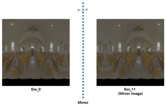
Figure 5.
Data augmentation using horizontal mirroring.
3.1.3. Rendered Images
Rendered images serve as conditions (y) for training the Latent Diffusion Model (LDM). Rendering was performed using the Mitsuba 3 Renderer. Each rendered image required one PBR map and one env map. However, exhaustively rendering all combinations (potentially 1.6 billion) was impractical due to computational limitations.
Therefore, for each PBR map, we randomly selected eight original (non-augmented) env maps for rendering. Augmented env maps were intentionally avoided to minimize model bias, as augmented versions share similar distributions. This process generated a final dataset of 320,000 pairs of [PBR map, env map, rendered image] used for training.
3.2. Model Training
Overall structure of proposed model is depicted in Figure 6.

Figure 6.
Overall architecture of proposed model. It has two PBR VAEs and env VAEs. In addition, the latent vectors (: 12 channels, : 3 channels) that passed through each encoder are concatenated and used as the input of the Latent U-Net. The rendered image is used as the condition of the U-Net.
3.2.1. PBR VAE
We implemented the PBR VAE using VQ-GAN [9], following a similar approach as MatFuse [4]. Each of the four PBR maps (basecolor, normal, roughness, metallic) was individually encoded into latent vectors of size . These four latent vectors were concatenated to form a combined latent vector (). A single unified decoder then reconstructed these latent representations back to their original maps.
The training loss function () combined pixel–space L2 loss, perceptual LPIPS loss, patch-based adversarial loss, codebook commitment loss, and rendering loss.
Training employed the Adam optimizer with mini-batch gradient descent, a batch size of 4, and a learning rate of . Training continued up to 120,000 iterations, until validation loss convergence.
3.2.2. ENV VAE
The env VAE was also based on VQ-GAN [9], structured with a single encoder–decoder pair. Env maps were compressed into latent representations () of size and then reconstructed.
The loss function included pixel–space L2 loss, perceptual LPIPS loss, patch-based adversarial loss, and codebook commitment loss (Excluding rendering loss from the loss function of Section 3.2.1).
Similar training parameters as the PBR VAE were applied—mini-batch gradient descent with Adam optimizer, batch size of 4, learning rate of , and 120,000 iterations.
The final architecture incorporating both VAEs is depicted in Figure 7.

Figure 7.
Structure of the two Variational Autoencoders (VAEs). The PBR encoder processes four types of basecolor (b), with normal (n), roughness (r), and metallic (m) as three separate channels, and concatenates them into one latent vector. The env encoder has a structure that encodes the env map into a three-channel latent vector () and concatenates it with . The decoder performs the above process in reverse.
3.2.3. Latent Diffusion Model (LDM)
Our generative model is based on the Latent Diffusion Model (LDM), which learns to reverse a forward diffusion process in a latent space. The LDM is trained to denoise a noisy latent vector conditioned on an input image y, which, in our case, is the rendered image. This process is guided by a UNet-based noise predictor, , which is optimized via the following objective function:
In this objective, the model (a UNet) is trained to predict the original noise from a noisy latent . The clean latent is produced by our pre-trained VAE, and the noisy latent is created by adding noise at a specific timestep t. The prediction is guided by the conditioning input y, which is processed into a vector sequence by a dedicated encoder and injected into the UNet via cross-attention.
The training utilizes the AdamW optimizer with a batch size of 32 and a learning rate of , continuing for 100,000 iterations. During inference, a linear schedule is used for , and noise is removed using the DDIM (Denoising Diffusion Implicit Model) sampling schedule.
4. Experiment
4.1. Evaluation Method
The primary objective of this study is to verify whether simultaneously generating PBR maps and environment maps (env maps) better preserves original PBR map characteristics compared to generating PBR maps alone. Specifically, we focus our evaluation on the basecolor map, as it is most significantly influenced by changes in the env map. To assess the similarity between the generated basecolor maps and the original maps, we employ the following three metrics:
- L-PIPSmeasures perceptual similarity by computing differences between deep feature maps obtained from pretrained vision models such as VGG-16. This metric effectively captures high-level visual similarities including textures, styles, and structures. An L-PIPS score closer to 0 indicates higher similarity between the two images.
- MS-SSIM is an extended version of the Structural Similarity Index Measure (SSIM), evaluating structural similarities at multiple scales. While SSIM comprehensively evaluates luminance, contrast, and structural similarity, MS-SSIM enhances this evaluation across various resolutions, providing a more robust measure of structural similarity. An MS-SSIM score closer to one indicates higher similarity.
- CIEDE2000 measures color difference based on the Lab color coordinates (L: luminance, a: green-to-red axis, b: blue-to-yellow axis). This metric accounts for human visual sensitivity to luminance, chroma, and hue. A higher CIEDE2000 value indicates a greater color difference. Generally, differences below three are barely noticeable or indistinguishable to the human eye, differences between three and six are clearly distinguishable, and differences above six are considered significantly noticeable.
For evaluation, each test PBR map was rendered with all 225 non-augmented test environment maps, generating 225 rendered images per PBR map. This procedure was consistently applied to 65 PBR maps, selecting five maps from each of the 13 test categories, producing a total of 14,625 rendered images. These images were then used as inputs to both our proposed model (EnvMat) and the baseline model (MatFuse) to generate respective PBR maps for comparison. The MatFuse model was trained on the identical dataset and iterations as the EnvMat model for a fair comparison.
4.2. Training Results
4.2.1. Baseline Model Reproduction
Prior to evaluating our proposed model, we first verified whether the baseline model was accurately reproduced. At the start of our research, only the source code of the baseline model was publicly available without any pretrained checkpoints. Additionally, the baseline model was originally trained on a different dataset than the one used in this study. Therefore, reproducing and validating the baseline model under identical training conditions is essential before proceeding with further comparisons.
To assess the quality of the reproduced baseline model, we evaluated the PBR maps (basecolor, roughness, normal, metallic) generated from the rendered images, employing the same quantitative metrics as the original study, namely FID-score and CLIP-IQA, along with qualitative assessments. These evaluations utilized rendered images created with an arbitrarily selected, identical env map to ensure consistency with the original paper.
Quantitatively, we measured FID-score and CLIP-IQA and compared our results (Table 1) with those of the original baseline study. For CLIP-IQA, we adopted the original high-quality and low-quality evaluation criteria. Notably, differences in CLIP-IQA scores between our reproduced model and the original baseline model are mainly attributed to differences in rendered image quality used for evaluation. CLIP-IQA heavily depends on the intrinsic quality of ground truth (GT) renderings. The rendered images employed in our study are of higher quality compared to those in the baseline study, as the MatSynth dataset utilized here is more recent and higher quality than the dataset used previously. Thus, our reproduced baseline model demonstrated CLIP-IQA scores close to the GT, indicating successful reproduction.

Table 1.
Baseline model reproduction. Quantitative evaluation comparing MatFuse (original paper), reproduced MatFuse (baseline), and proposed EnvMat model.
However, our reproduced model showed relatively higher differences in the FID-score compared to the original baseline. This difference is primarily due to the original model being trained on a larger dataset with substantially more training iterations. Specifically, our model was trained with 320,000 (PBR-rendered image) pairs for 120,000 (VAE) and 100,000 (LDM) iterations, whereas the baseline study trained with approximately ten times more data, consisting of 3,200,000 pairs for over 4,000,000 (VAE) and 500,000 (LDM) iterations. Given these considerable differences in training data volume and iterations, it is natural that the original baseline model achieved superior FID-scores.
The training process for this study was terminated early when the loss function converged. The reason for the lower number of training iterations compared to the MatFuse paper is a natural consequence of our dataset size being approximately one-tenth of theirs. Due to computational resource and time constraints, it was not feasible to preprocess and train on data at the same scale as MatFuse. Consequently, our model’s loss converged within fewer iterations, which can be interpreted as an aspect of training efficiency.
Additionally, the quantitative comparative experiments in the Appendix A (Figure A1–Figure A7) confirm that the reproduced MatFuse produces results at a level suitable for the experiments.
Despite these differences, our reproduced baseline model achieved satisfactory results both quantitatively and qualitatively, verifying its suitability for comparative evaluation with our proposed model (EnvMat).
4.2.2. Qualitative Evaluation
The figures in the Appendix A (Figure A8–Figure A21) illustrate comparisons of basecolor maps generated by the proposed EnvMat and the baseline MatFuse model. Each figure includes the same original PBR map (top-left in the first row), rendered images using different env maps (top-right in the first row and second row), and the resulting basecolor maps generated by EnvMat (third row, left) and MatFuse (third row, right).
In the rendered images, significant color distortion due to different environment maps is evident when compared to the original basecolor maps. Observing the generated outputs, EnvMat consistently produced basecolor maps whose colors closely matched the original, while MatFuse exhibited noticeable deviations.
These qualitative results suggest that MatFuse tends to reflect the distorted color information from rendered images rather than the original basecolor map. In contrast, EnvMat effectively mitigates color distortions from heavily altered rendered images, producing results closer to the original basecolor maps.
4.2.3. Quantitative Evaluation
To verify the effectiveness of our proposed model, we performed a quantitative evaluation that also served as an ablation study for our primary contribution. We compared our EnvMat model against the MatFuse architecture under identical training and evaluation conditions. Since the MatFuse architecture was equivalent to our EnvMat model with the Environment Map VAE (env VAE) component removed, this comparison directly isolates and measures the impact of simultaneously generating environment maps.
We quantitatively evaluated our results using the metrics L-PIPS, MS-SSIM, and CIEDE2000. Following the evaluation protocol described in Section 4.1, we calculated the average similarity scores between the 14,625 basecolor maps generated from each model and their corresponding original basecolor maps. Table 2 summarizes the results.
Table 2.
Quantitative comparison between EnvMat (our model) and MatFuse (baseline).
The results in Table 2 clearly validate our approach. Interpreted as an ablation study, the significant performance drop observed in the MatFuse model across all metrics, especially the 10-point degradation in the CIEDE2000 color accuracy score, directly demonstrates that the env VAE is essential for preserving color fidelity. As a comparison to the baseline architecture, EnvMat sets a new performance benchmark, confirming that our method of simultaneous generation yields basecolor maps more closely aligned with the original.
4.3. Performance Analysis
To evaluate the practical applicability of our proposed model, we analyzed its real-time performance in terms of inference time and memory usage, as requested by the reviewer. We measured the average time required to generate a single output and the peak GPU memory consumption during inference. Both EnvMat and the MatFuse baseline were evaluated on the same NVIDIA A6000 GPU (Nvidia Corporation, Santa Clara, CA, USA). The results are summarized in Table 3.
Table 3.
Inference time and memory usage comparison.
The analysis reveals a compelling finding—despite utilizing an additional VAE for environment maps, EnvMat exhibits a comparable inference time to the baseline. Furthermore, the increase in memory usage is approximately 266 MiB, a negligible overhead of about 3.2%. These results demonstrate that our method achieves a significant improvement in output quality and color fidelity, with almost no additional computational cost. This highlights the efficiency of our approach and its strong potential for practical applications.
5. Conclusions and Future Work
5.1. Conclusions
Based on the experimental results presented in Section 4, we demonstrate that the proposed EnvMat model, which simultaneously generates environment maps and PBR maps, consistently produced outputs closer to the original maps compared to the baseline model, which generates only PBR maps. Our qualitative and quantitative evaluations confirm that EnvMat achieved superior performance in terms of L-PIPS and MS-SSIM metrics. Particularly, EnvMat showed significant improvement in the CIEDE2000 metric, achieving differences greater than six, indicating clearly distinguishable enhancements in color fidelity.
These results confirm that simultaneously predicting env maps alongside PBR maps significantly mitigates color distortions introduced by varying environmental lighting, effectively preserving the original characteristics of the PBR maps.
Furthermore, our performance analysis revealed that these significant quality improvements are achieved with negligible additional computational cost, highlighting the efficiency and practical viability of our approach.
5.2. Limitations
This study acknowledges that the environment map dataset used was limited to indoor scenes, which restricts the model’s generalizability across diverse environments. This was primarily due to the practical availability of suitable datasets during the research period.
Furthermore, a significant difference in training data scale exists when comparing our work to the original MatFuse baseline paper. While the MatFuse paper trained on a 3.2M-scale dataset, our experiments were conducted with approximately one-tenth of that data. This was a consequence of physical limitations encountered during data preprocessing; the rendering of corresponding images for each material and environment map proved to be exceptionally time-consuming and computationally intensive. Due to these resource constraints, training on a scale equivalent to MatFuse was not feasible within the scope of the current research.
Our qualitative analysis revealed that the model struggled to accurately reproduce reddish-toned lighting environments (Figure A22 and Figure A23). We attribute this primarily to an imbalance in the training data distribution.
Recognizing this challenge, we reproduced the MatFuse model using an equivalently scaled dataset to our own. This allowed for a direct comparison between the reproduced MatFuse model and our proposed model. The results clearly demonstrated a significant performance enhancement, particularly in color fidelity, as our framework achieved a remarkable improvement of over six in the CIEDE2000 metric.
In real-world physical environments, purely red ambient light conditions are exceptionally rare, especially when compared to common lighting scenarios like sunsets (which are more orange) or general illumination. Consequently, the vast majority of publicly available environment map datasets do not contain a sufficient number of these reddish-toned environments.
As a result, our model, having been trained on a limited amount of reddish-toned data, exhibited poor generalization performance in this color space, tending to produce inaccurate colors or artifacts. To address this, data augmentation strategies involving the intentional rendering of reddish-toned environments would be necessary. While beyond the scope of this paper, this represents a crucial direction for future research to enhance the model’s robustness.
5.3. Future Work
To build upon our findings, we propose the following directions for future research:
- Increased Generalization through Expanded Datasets: Future research should employ larger and more diverse datasets to further enhance the model’s generalization capability. Expanding the training dataset with additional MatSynth materials, env maps featuring diverse color distributions, as well as env maps captured from various environments (including outdoor and studio lighting conditions), will substantially improve the robustness and applicability of the proposed model.
- Incorporation of Render Loss in UNet Training: While Render Loss is often beneficial for optimizing physically based rendering (PBR) assets by evaluating the difference between rendered outputs generated from predicted maps and original renderings, its direct application to our Latent UNet architecture presents inherent structural challenges. Render Loss operates by comparing renderings at the pixel level. However, our Latent UNet operates and generates representations within a latent space, not the pixel space, thereby preventing the direct rendering of intermediate PBR and environment maps for Render Loss computation during its training. Although this loss was effectively employed during VAE training, its integration into the UNet training process remains a significant challenge. This characteristic is common in Latent Diffusion Models. Consistent with the previous work utilizing UNets in similar latent spaces, we did not employ Render Loss during UNet training. Future research should explore methods to effectively integrate Render Loss into UNet training, which could lead to even closer alignment with original renderings and potentially further improve the accuracy of generated results.
Author Contributions
Conceptualization, S.O.; methodology, S.O. and M.J.; software, S.O.; validation, S.O. and T.K.; formal analysis, S.O.; investigation, T.K.; resources, M.J.; data curation, S.O.; writing—original draft preparation, S.O.; writing—review and editing, T.K.; visualization, S.O.; supervision, T.K.; project administration, T.K.; funding acquisition, T.K. All authors have read and agreed to the published version of the manuscript.
Funding
This research was supported by IITP and MSIT of Korea through the Graduate School of Metaverse Convergence Program (RS-2022-00156318), and by MCST of Korea through the KOCCA grant (RS-2023-00219237) as part of the Culture, Sports, and Tourism R&D Program.
Data Availability Statement
The original data presented in the study are openly available in MatSynth at https://huggingface.co/datasets/gvecchio/MatSynth.
Conflicts of Interest
The authors declare no conflicts of interest.
Appendix A
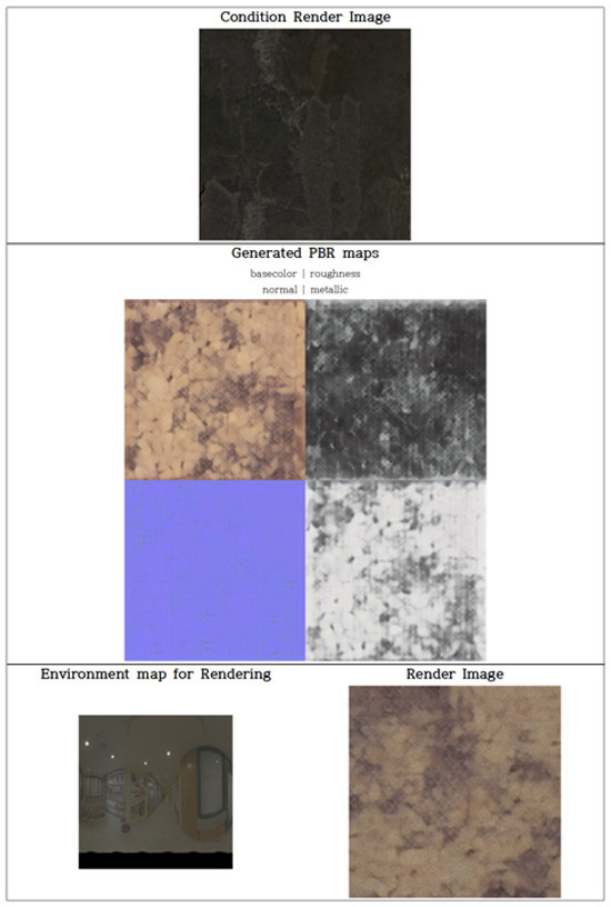
Figure A1.
Reproduced MatFuse results. The PBR map (row 2) generated via Condition Render Image (row 1) and the Render Image (row 3, column 2) rendered with a randomly selected env map (row 3, column 1).
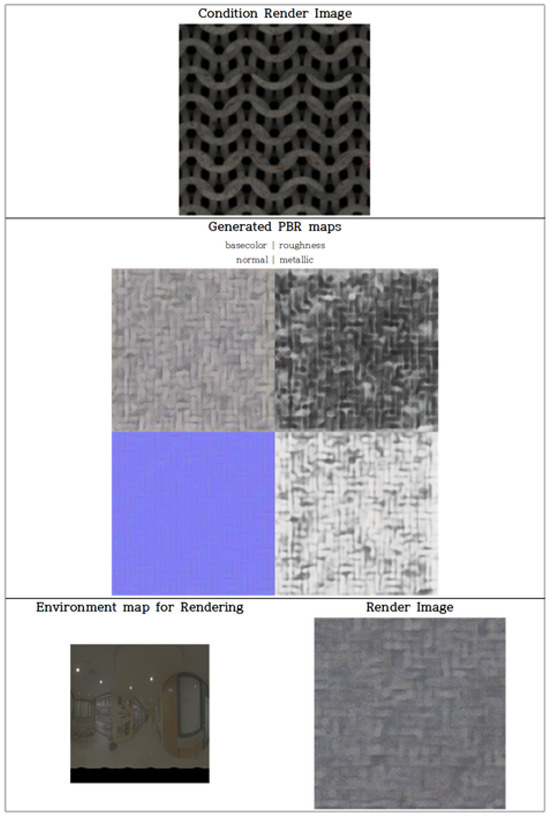
Figure A2.
Reproduced MatFuse results. The PBR map (row 2) generated via Condition Render Image (row 1) and the Render Image (row 3, column 2) rendered with a randomly selected env map (row 3, column 1).
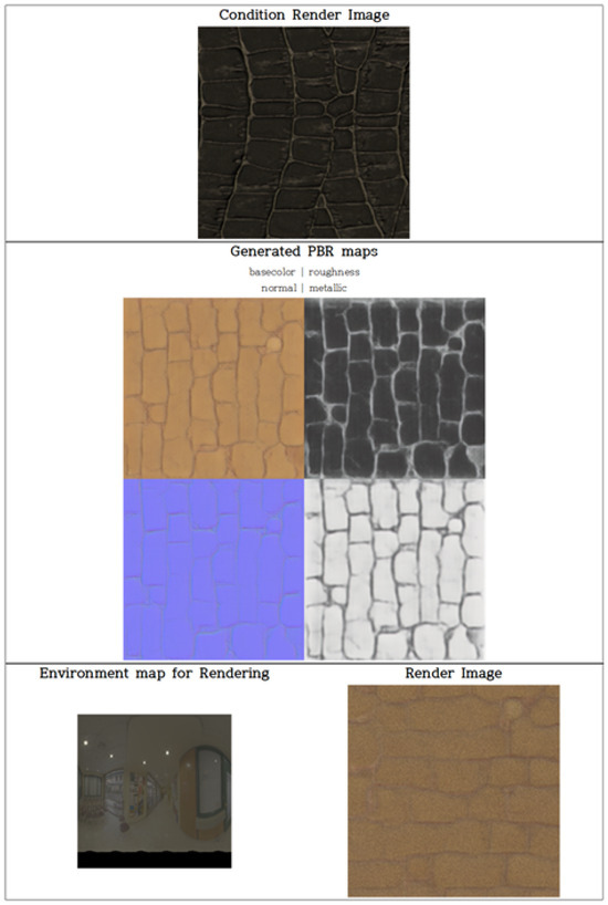
Figure A3.
Reproduced MatFuse results. The PBR map (row 2) generated via Condition Render Image (row 1) and the Render Image (row 3, column 2) rendered with a randomly selected env map (row 3, column 1).
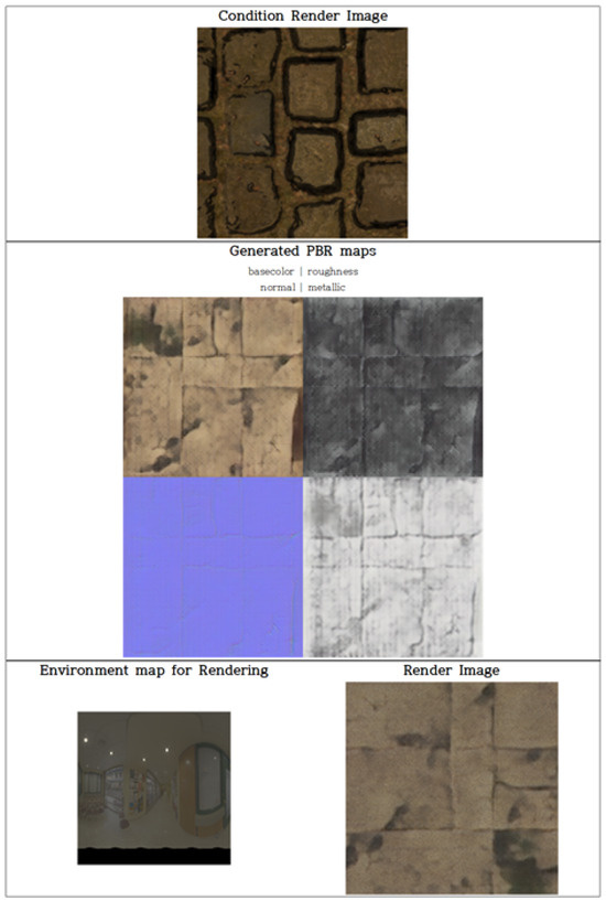
Figure A4.
Reproduced MatFuse results. The PBR map (row 2) generated via Condition Render Image (row 1) and the Render Image (row 3, column 2) rendered with a randomly selected env map (row 3, column 1).

Figure A5.
Reproduced MatFuse results. The PBR map (row 2) generated via Condition Render Image (row 1) and the Render Image (row 3, column 2) rendered with a randomly selected env map (row 3, column 1).
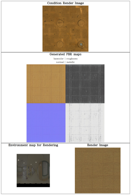
Figure A6.
Reproduced MatFuse results. The PBR map (row 2) generated via Condition Render Image (row 1) and the Render Image (row 3, column 2) rendered with a randomly selected env map (row 3, column 1).
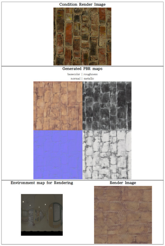
Figure A7.
Reproduced MatFuse results. The PBR map (row 2) generated via Condition Render Image (row 1) and the Render Image (row 3, column 2) rendered with a randomly selected env map (row 3, column 1).
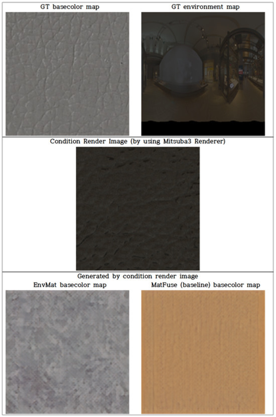
Figure A8.
Comparison of inference results of EnvMat (3 rows, 1 column) and MatFuse (3 rows, 2 columns). Inference results using the Condition render image (2 rows) generated from the same PBR map (1 row, 1 column) and env map (1 row, 2 columns) as input.

Figure A9.
Comparison of inference results of EnvMat (3 rows, 1 column) and MatFuse (3 rows, 2 columns). Inference results using the Condition render image (2 rows) generated from the same PBR map (1 row, 1 column) and env map (1 row, 2 columns) as input.
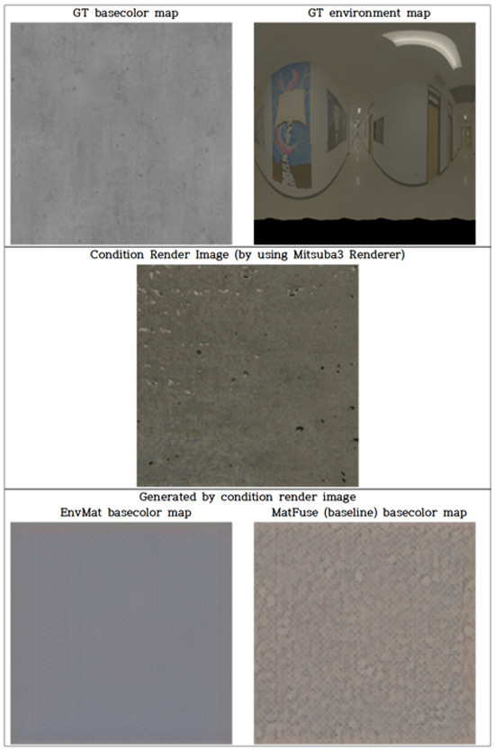
Figure A10.
Comparison of inference results of EnvMat (3 rows, 1 column) and MatFuse (3 rows, 2 columns). Inference results using the Condition render image (2 rows) generated from the same PBR map (1 row, 1 column) and env map (1 row, 2 columns) as input.
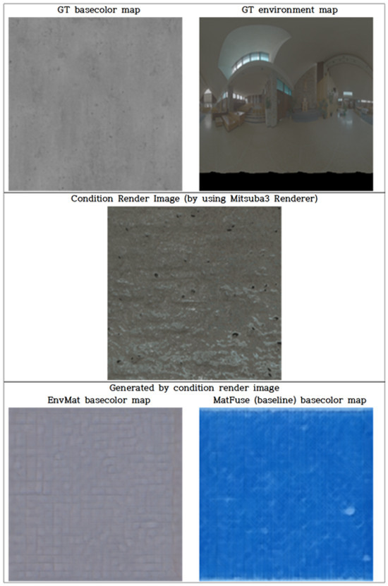
Figure A11.
Comparison of inference results of EnvMat (3 rows, 1 column) and MatFuse (3 rows, 2 columns). Inference results using the Condition render image (2 rows) generated from the same PBR map (1 row, 1 column) and env map (1 row, 2 columns) as input.
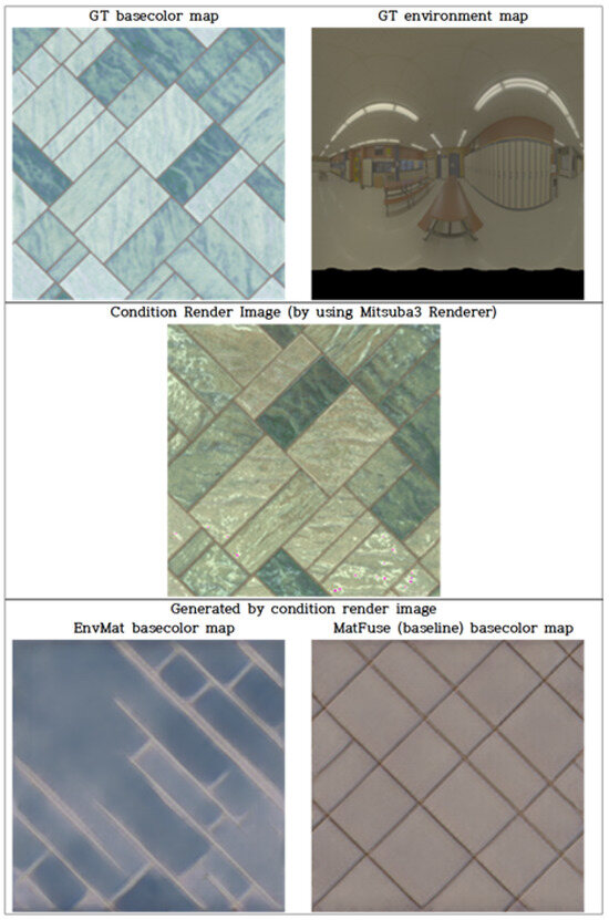
Figure A12.
Comparison of inference results of EnvMat (3 rows, 1 column) and MatFuse (3 rows, 2 columns). Inference results using the Condition render image (2 rows) generated from the same PBR map (1 row, 1 column) and env map (1 row, 2 columns) as input.
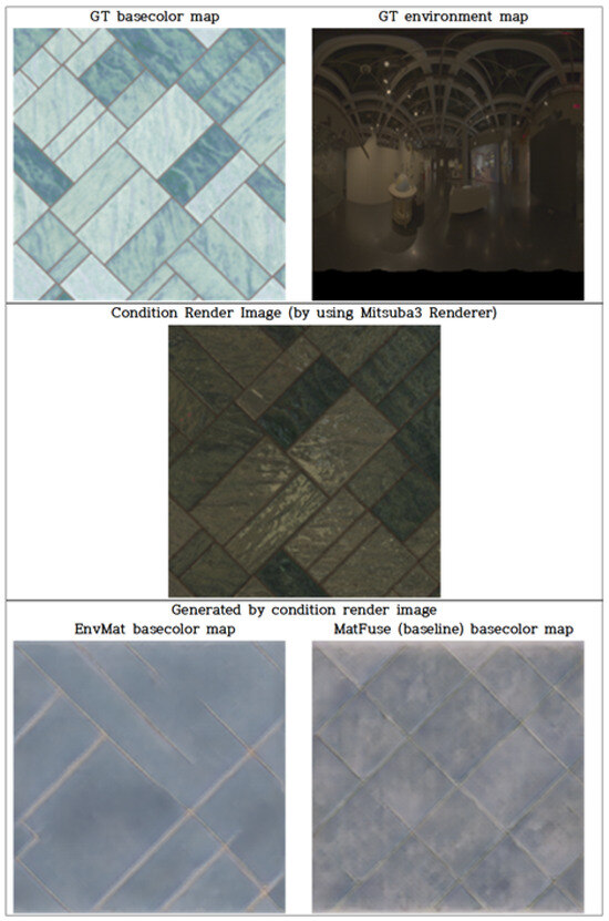
Figure A13.
Comparison of inference results of EnvMat (3 rows, 1 column) and MatFuse (3 rows, 2 columns). Inference results using the Condition render image (2 rows) generated from the same PBR map (1 row, 1 column) and env map (1 row, 2 columns) as input.
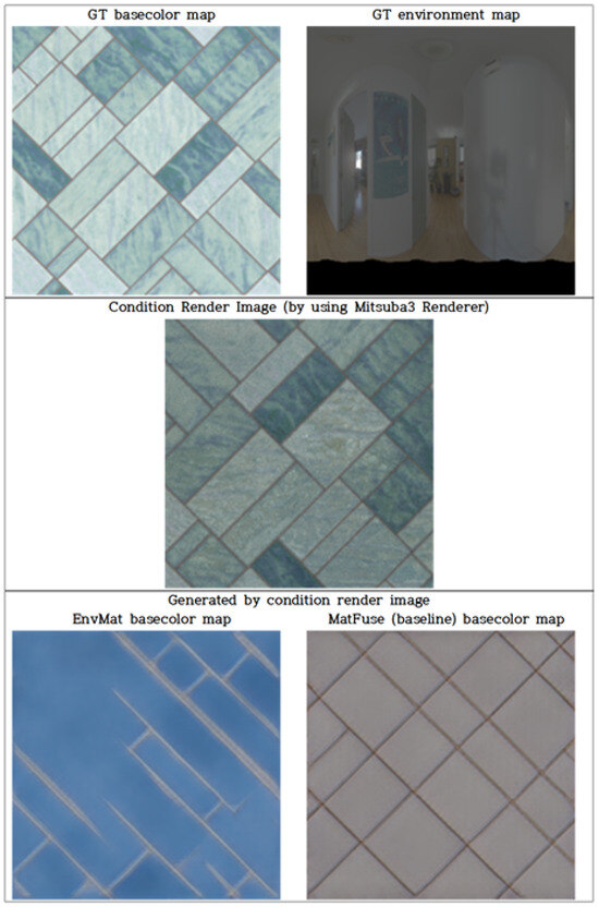
Figure A14.
Comparison of inference results of EnvMat (3 rows, 1 column) and MatFuse (3 rows, 2 columns). Inference results using the Condition render image (2 rows) generated from the same PBR map (1 row, 1 column) and env map (1 row, 2 columns) as input.
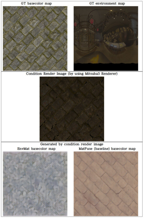
Figure A15.
Comparison of inference results of EnvMat (3 rows, 1 column) and MatFuse (3 rows, 2 columns). Inference results using the Condition render image (2 rows) generated from the same PBR map (1 row, 1 column) and env map (1 row, 2 columns) as input.
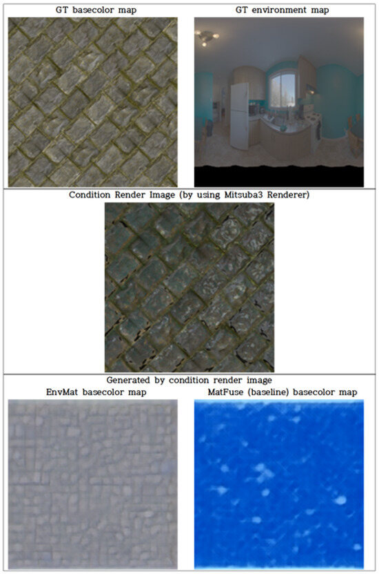
Figure A16.
Comparison of inference results of EnvMat (3 rows, 1 column) and MatFuse (3 rows, 2 columns). Inference results using the Condition render image (2 rows) generated from the same PBR map (1 row, 1 column) and env map (1 row, 2 columns) as input.
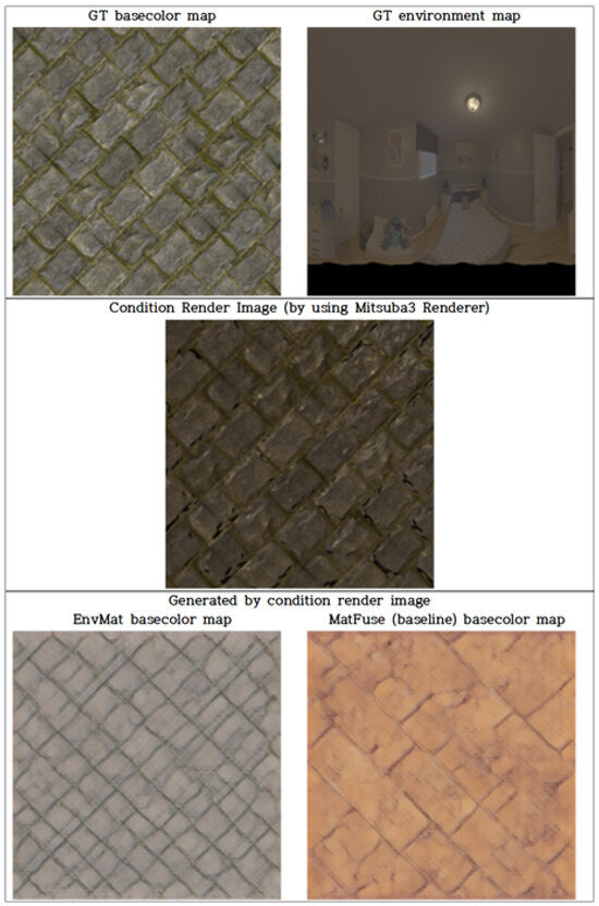
Figure A17.
Comparison of inference results of EnvMat (3 rows, 1 column) and MatFuse (3 rows, 2 columns). Inference results using the Condition render image (2 rows) generated from the same PBR map (1 row, 1 column) and env map (1 row, 2 columns) as input.
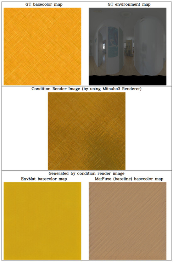
Figure A18.
Comparison of inference results of EnvMat (3 rows, 1 column) and MatFuse (3 rows, 2 columns). Inference results using the Condition render image (2 rows) generated from the same PBR map (1 row, 1 column) and env map (1 row, 2 columns) as input.
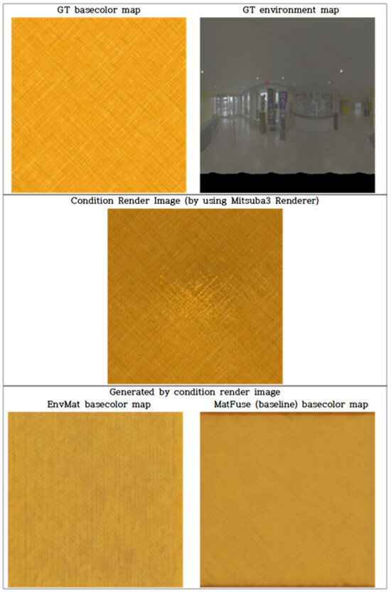
Figure A19.
Comparison of inference results of EnvMat (3 rows, 1 column) and MatFuse (3 rows, 2 columns). Inference results using the Condition render image (2 rows) generated from the same PBR map (1 row, 1 column) and env map (1 row, 2 columns) as input.
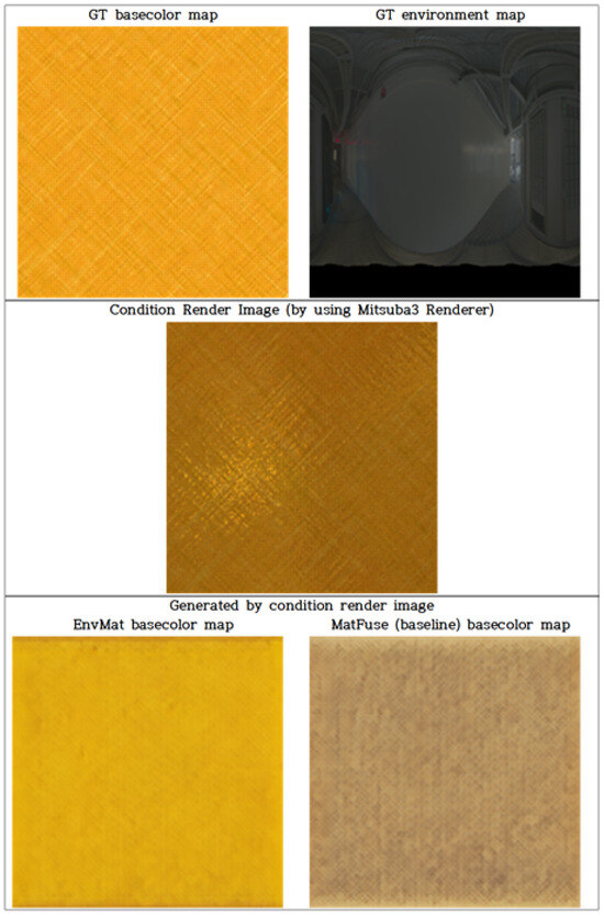
Figure A20.
Comparison of inference results of EnvMat (3 rows, 1 column) and MatFuse (3 rows, 2 columns). Inference results using the Condition render image (2 rows) generated from the same PBR map (1 row, 1 column) and env map (1 row, 2 columns) as input.
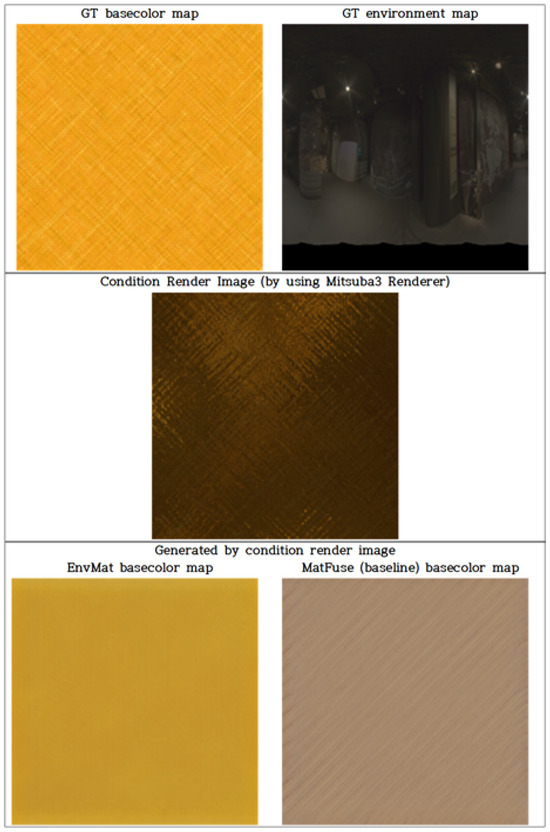
Figure A21.
Comparison of inference results of EnvMat (3 rows, 1 column) and MatFuse (3 rows, 2 columns). Inference results using the Condition render image (2 rows) generated from the same PBR map (1 row, 1 column) and env map (1 row, 2 columns) as input.
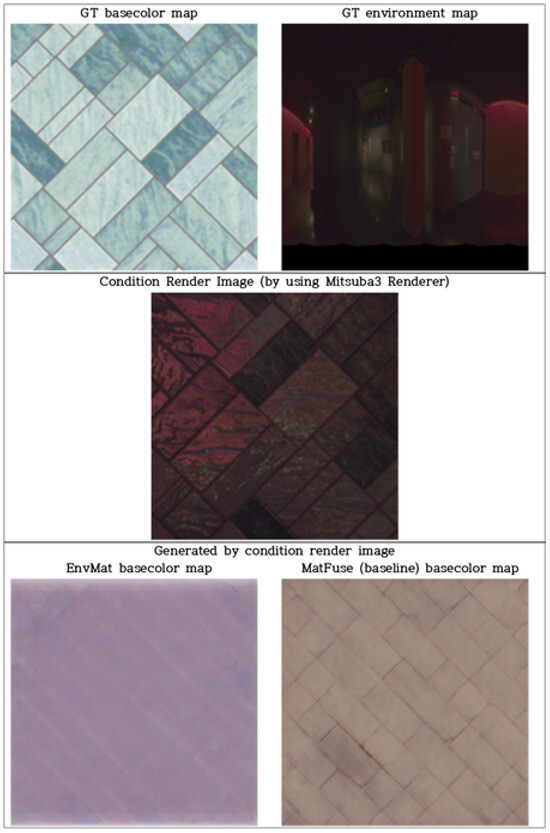
Figure A22.
Limitations: Comparison of inference results of EnvMat (3 rows, 1 column) and MatFuse (3 rows, 2 columns). Inference results using the Condition render image (2 rows) generated from the same PBR map (1 row, 1 column) and env map (1 row, 2 columns) as input.
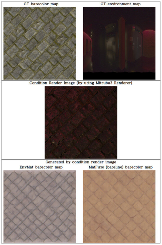
Figure A23.
Limitations: Comparison of inference results of EnvMat (3 rows, 1 column) and MatFuse (3 rows, 2 columns). Inference results using the Condition render image (2 rows) generated from the same PBR map (1 row, 1 column) and env map (1 row, 2 columns) as input.
References
- Krizhevsky, A.; Sutskever, I.; Hinton, G.E. ImageNet Classification with Deep Convolutional Neural Networks. In Proceedings of the Advances in Neural Information Processing Systems 25, Lake Tahoe, NV, USA, 3–6 December 2012; pp. 1097–1105. [Google Scholar]
- Karras, T.; Laine, S.; Aittala, M.; Hellsten, J.; Lehtinen, J.; Aila, T. Analyzing and Improving the Image Quality of StyleGAN. In Proceedings of the IEEE/CVF Conference on Computer Vision and Pattern Recognition (CVPR), Seattle, WA, USA, 13–19 June 2020; pp. 8110–8119. [Google Scholar]
- Rombach, R.; Blattmann, A.; Lorenz, D.; Esser, P.; Ommer, B. High-Resolution Image Synthesis with Latent Diffusion Models. In Proceedings of the the IEEE/CVF Conference on Computer Vision and Pattern Recognition (CVPR), New Orleans, LA, USA, 18–24 June 2022; pp. 10684–10695. [Google Scholar]
- Vecchio, G.; Sortino, R.; Palazzo, S.; Spampinato, C. MatFuse: Controllable Material Generation with Diffusion Models. In Proceedings of the IEEE/CVF Conference on Computer Vision and Pattern Recognition (CVPR), Seattle, WA, USA, 16–22 June 2024; pp. 4429–4438. [Google Scholar]
- Deschaintre, V.; Aittala, M.; Durand, F.; Drettakis, G.; Bousseau, A. Single-Image SVBRDF Capture with a Rendering-Aware Deep Network. ACM Trans. Graph. 2018, 37, 128:1–128:15. [Google Scholar] [CrossRef]
- Vecchio, G.; Palazzo, S.; Spampinato, C. SurfaceNet: Adversarial SVBRDF Estimation from a Single Image. In Proceedings of the IEEE/CVF International Conference on Computer Vision (ICCV), Montreal, BC, Canada, 11–17 October 2021; pp. 12840–12848. [Google Scholar]
- Guo, Y.; Smith, C.; Hašan, M.; Sunkavalli, K.; Zhao, S. MaterialGAN: Reflectance Capture Using a Generative SVBRDF Model. ACM Trans. Graph. 2020, 39, 254:1–254:13. [Google Scholar] [CrossRef]
- Dhariwal, P.; Nichol, A. Diffusion Models Beat GANs on Image Synthesis. In Proceedings of the Advances in Neural Information Processing Systems 34, Virtual, 6–14 December 2021; pp. 8780–8794. [Google Scholar]
- Esser, P.; Rombach, R.; Ommer, B. Taming Transformers for High-Resolution Image Synthesis. In Proceedings of the IEEE/CVF Conference on Computer Vision and Pattern Recognition (CVPR), Nashville, TN, USA, 20–25 June 2021; pp. 12873–12883. [Google Scholar]
- He, Z.; Guo, J.; Zhang, Y.; Tu, Q.; Chen, M.; Guo, Y.; Wang, P.; Dai, W. Text2Mat: Generating Materials from Text. In Proceedings of the Pacific Graphics 2023—Short Papers and Posters, Daejeon, Republic of Korea, 10–13 October 2023; pp. 89–97. [Google Scholar]
- Martin, R.; Roullier, A.; Rouffet, R.; Kaiser, A.; Boubekeur, T. MaterIA: Single Image High-Resolution Material Capture in the Wild. Comput. Graph. Forum 2022, 41, 163–177. [Google Scholar] [CrossRef]
- Vecchio, G.; Martin, R.; Roullier, A.; Kaiser, A.; Rouffet, R.; Deschaintre, V.; Boubekeur, T. ControlMat: A Controlled Generative Approach to Material Capture. ACM Trans. Graph. 2024, 43, 164:1–164:17. [Google Scholar] [CrossRef]
- Vecchio, G.; Deschaintre, V. MatSynth: A Modern PBR Materials Dataset. In Proceedings of the IEEE/CVF Conference on Computer Vision and Pattern Recognition (CVPR), Seattle, WA, USA, 16–22 June 2024; pp. 22109–22118. [Google Scholar]
- Laval Indoor HDR Environment Map Dataset. 2014. Available online: http://hdrdb.com/indoor/ (accessed on 12 May 2025).
- Chung, H.; Kim, J.; McCann, M.T.; Klasky, M.L.; Ye, J.C. Diffusion Posterior Sampling for General Noisy Inverse Problems. arXiv 2022, arXiv:2209.14687. [Google Scholar]
Disclaimer/Publisher’s Note: The statements, opinions and data contained in all publications are solely those of the individual author(s) and contributor(s) and not of MDPI and/or the editor(s). MDPI and/or the editor(s) disclaim responsibility for any injury to people or property resulting from any ideas, methods, instructions or products referred to in the content. |
© 2025 by the authors. Licensee MDPI, Basel, Switzerland. This article is an open access article distributed under the terms and conditions of the Creative Commons Attribution (CC BY) license (https://creativecommons.org/licenses/by/4.0/).