Article

Enhancing Spectrum Utilization in Cognitive Radio Networks Using Reinforcement Learning with Snake Optimizer: A Meta-Heuristic Approach

by
Haider Farhi
1,*,
Abderraouf Messai
1 and
Tarek Berghout
2
1
Laboratoire Satellite, Intelligence Artificielle, Cryptographie et Internet des Objets (SIACIO), Department of Electronics, University of Constantine 1—Frères Mentouri, Route Ain El Bey, Constantine 25000, Algeria
2
Department of Industrial Engineering, Faculty of Technology, University of Batna 2, Batna 05000, Algeria
*
Author to whom correspondence should be addressed.
Electronics 2025, 14(13), 2525; https://doi.org/10.3390/electronics14132525
Submission received: 25 May 2025 / Revised: 16 June 2025 / Accepted: 17 June 2025 / Published: 21 June 2025

Abstract

The rapid development of sixth-generation mobile communication systems has brought about significant advancements in both Quality of Service (QoS) and Quality of Experience (QoE) for users, largely due to the extremely high data rates and a diverse range of service offerings. However, these advancements have also introduced challenges, especially concerning the growing demand for a wireless spectrum and the limited availability of resources. Various efforts have been made and research has attempted to tackle this issue such as the use of Cognitive Radio Networks (CRNs), which allows opportunistic spectrum access and intelligent resource management. This work demonstrate a new method in the optimization of allocation resource in CRNs based on the Snake Optimizer (SO) along with reinforcement learning (RL), which is an effective meta-heuristic algorithm that simulates snake cloning behavior. SO is tested over three different scenarios with varying numbers of secondary users (SUs), primary users (PUs), and frequency bands available. The obtained results reveal that the proposed approach is able to largely satisfy the aforementioned requirements and ensures high spectrum utilization efficiency and low collision rates, which eventually lead to the maximum possible spectral capacity. The study also demonstrates that SO is versatile and resilient and thus indicates its capability of serving as an effective method for augmenting resource management in next-generation wireless communication systems.

1. Introduction

With the deployment of sixth-generation mobile communication systems, users benefit from improved QoS and a wide range of high-quality services delivered at extremely high data rates [1]. However, despite these advancements, significant challenges remain (notably the explosive growth in data traffic and the scarcity of available spectrum resources [2]). The increasing demand for wireless applications and the inefficient utilization of the radio spectrum highlight the urgent need for innovative solutions, one of which is the implementation of cognitive radio (CR) technology.
Recently, CR has gained considerable attention from both the industry and academia as a promising technology for dynamic spectrum management to increase the reliability and throughput of wireless communication systems. CRNs are intelligent wireless systems in which SUs, equipped with cognitive capabilities, dynamically adapt their transmission parameters based on the surrounding radio environment. This promotes a more dynamic and resource-efficient application of the available spectrum without interfering with licensed PUs [3]. In addition to spectrum sensing and access, CR introduces intelligent mechanisms for spectrum management and interference mitigation by analyzing and adapting to various communication scenarios [4,5].
CR is an emerging paradigm for radio spectrum allocation that enables SUs to exploit underutilized transmission opportunities in the licensed spectrum, provided that their transmissions do not degrade those of PUs [6]. CRNs typically operate under three primary access models: (i) the underlay model, (ii) the overlay model, and (iii) a hybrid of the two. In the underlay model, concurrent transmission by SUs and PUs is permitted, given that the interference caused to PUs remains below a predetermined benchmark, commonly known as Interference Temperature, that defines acceptable interference levels [7]. In the overlay model, SUs exploit unused spectral bands not currently accessed by PUs, often using advanced signal processing or cooperation techniques. The hybrid model combines features of both. Among these, the underlay model is often preferred for its simplicity and efficient spectrum utilization, along with lower implementation complexity compared to the hybrid approach [8].
A significant number of recent studies have shown that spectrum utilization in underlay CRNs can be greatly enhanced through efficient resource allocation strategies. In such systems, the coexistence of Primary Base Stations (PBSs) and Secondary Base Stations (SBSs) introduces a major challenge known as Co-Channel Interference (CCI), which is a primary bottleneck in resource allocation. When PBSs and SUs utilize the same subchannel concurrently, severe CCI can occur due to three main interference sources: (i) interference from PUs to SUs, (ii) interference between SU-PU communication links and other devices, and (iii) interference among SUs themselves [9]. While the first type of interference is typically managed by setting a suitable threshold to ensure QoS for PUs, the other types are addressed through orthogonal transmission schemes, power control strategies, and interference constraints [10].
This study aims to mitigate CCI by designing optimal resource allocation strategies that include channel selection and power control. Optimization theory and heuristic algorithms are two main approaches used to model and solve resource allocation problems in CRNs.
For example, in [11], the authors conducted a study on optimizing energy-efficient resource distribution in CRNs employing Orthogonal Frequency Division Multiplexing (OFDM) technology by formulating a non-linear fractional programming problem, which was solved using a time-sharing approach to achieve near-optimal solutions. In [12], the authors proposed an approach to optimize the weighted sum rate for users transmitting orthogonally, modeling the problem as a non-convex optimization challenge and solving it with Channel State Information (CSI) from both primary and secondary systems using Lagrange multipliers. Similarly, Ref. [13] addressed an optimization problem focused on energy efficiency involving resource and power allocation for Orthogonal Frequency-Division Multiple Access (OFDMA)-based hybrid CRNs, deriving closed-form solutions using the Lagrange dual decomposition method. Additionally, the study in [14] introduced a modified Ant Colony Optimization algorithm inspired by the foraging behavior of ants to solve the resource allocation problem in CRNs. Furthermore, the work in [15] presented a dynamic Medium Access Control (MAC) framework and optimal resource allocation strategy for multi-channel ad hoc CRNs, optimized using the Particle Swarm Optimization (PSO) algorithm.
Despite these advancements, resource allocation in CRNs remains a complex and challenging task, often classified as NP-hard and typically yielding only near-optimal solutions [16]. In real-time operations, the limitations of globally constrained optimization become apparent due to high computational time and complexity. To address these challenges, CR users are expected to leverage learning capabilities to identify optimal strategies for CRNs. Recent progress in Artificial Intelligence (AI), especially in Machine Learning (ML) and RL, offers promising solutions for achieving efficient resource management strategies [17,18,19].
The study in [20] proposed an online Q-learning scheme for power allocation, where cognitive users employ predictive features to identify the power level that maximizes performance under given constraint. Another study in [21] introduced an asynchronous Advantage Actor-Critic (A3C)-based power control scheme for SUs, in which SUs learn power control policies concurrently across multiple CPU threads, reducing the interdependency of neural network gradient updates. Additionally, RL techniques have gained popularity in multi-agent environments and distributed systems. For instance, Ref. [22] presented a multi-agent model-free RL scheme for resource allocation, which mitigates interference and eliminates the need for a network model through decentralized cooperative learning.
While RL has demonstrated its potential in enabling both PUs and SUs in CRNs to intelligently manage resources, its performance tends to degrade significantly as the scale of the wireless communication network increases [23]. This degradation is primarily due to RL algorithms typically representing the network state using Euclidean data structures, such as CSI matrices and user request matrices, which fail to fully capture the underlying topology of wireless networks. To address this limitation, recent research has focused on incorporating topological information to enable more effective learning.
For instance, the study in [24] explored the application of spatial convolution techniques for scheduling in the context of the sum-rate maximization model, leveraging user location data. They proposed a novel graph embedding-based approach for link scheduling in Device-To-Device (D2D) networks, utilizing a K-Nearest Neighbor (KNN) graph representation method to reduce computational complexity.
Due to its cognitive capabilities, a CR can interact with its environment in real time, enabling it to identify and adjust optimal communication parameters as the radio environment evolves. In essence, CR systems continuously analyze environmental data to determine the best possible transmission parameters that meet specific performance requirements. The accuracy of decisions made by CR systems is highly influenced by how the environmental input is represented. Furthermore, the selection of transmission parameters plays a critical role in determining overall spectral efficiency. In the literature, meta-heuristic approaches have effectively tackled the challenges of dynamic CR parameter adaptation.
The structure of this paper is as follows: Section 2, Related Works, reviews the existing literature on cognitive radio networks, spectrum utilization strategies, reinforcement learning, and meta-heuristic optimization techniques, identifying key challenges and research gaps. Section 3, Proposed Methodology, presents the system model and introduces a novel framework that integrates reinforcement learning with the Snake Optimizer to enhance spectrum decision-making in dynamic environments. Section 4 also explains the design and functioning of the Snake Optimizer, inspired by the natural behavior of snakes, and its role in improving the learning efficiency of the cognitive radio system. Section 5, Results and Discussion, provides experimental validation of the proposed approach across multiple scenarios, comparing its performance with traditional methods and discussing the implications of the results. Finally, Section 6, Conclusions, summarizes the key findings, highlights the contributions of the study, and outlines potential directions for future research in intelligent spectrum management.

2. Related Works

Meta-heuristic algorithms have garnered significant attention because of their simplicity of implementation, high convergence rates, and robust capabilities in solving complex optimization problems, including non-linear, mixed-variable, and constrained problems [25]. Typically, these algorithms begin with a randomly generated population of solutions, which are iteratively refined. What differentiates one meta-heuristic algorithm from another is the method used to update or modify these candidate solutions during the optimization process. In the context of Cognitive Dynamic Environments (CDEs), meta-heuristics have proven effective for dynamic parameter adaptation, with over two decades of research dedicated to this field. CDE optimization has been explored using various meta-heuristic algorithms, such as Genetic Algorithms (GAs) [26], PSO [27], Artificial Bee Colony (ABC) algorithms [28], Ant Colony Optimization (ACO) [29], Simulated Annealing (SA), Biogeography-Based Optimization (BBO) [30], and Cat Swarm Optimization (CSO). This work specifically focuses on leveraging these techniques to enhance parameter adaptation in CDEs.
For instance, Newman et al. [26] proposed a GA-based approach to optimize transmission parameters in both single- and multi-carrier CR systems. Their method used a weighted sum strategy to simultaneously optimize multiple fitness functions, adjusting parameters such as power levels and modulation schemes. However, GA often suffered from local optima traps and required around 500 iterations to reach convergence. Zhao et al. [27] employed PSO to adapt parameters in a multi-carrier cognitive radio setup under a Multi-Objective Optimization (MOO) framework. The PSO algorithm showed superior performance over GA in terms of fitness values and solution stability across four operational modes. A comparative study by Pradhan et al. [28] evaluated GA, PSO, and ABC algorithms in optimizing CDEs across three transmission modes, while respecting interference constraints: low-power, multimedia, and emergency. Their results showed that ABC outperformed both GA and PSO in terms of average fitness and computation time. Zhao et al. [29] also introduced a Mutated Ant Colony Optimization (MACO) algorithm designed for CDE optimization involving 10 subcarriers. The mutation mechanism in MACO helped escape local minima and yielded superior performance, particularly under a 0.9 pheromone evaporation rate, outperforming both GA and traditional ACO. Kaur et al. [30] proposed an SA-based method to optimize transmission parameters while meeting stringent QoS constraints like minimizing power, reducing bit error rates, and improving throughput and spectral efficiency. Although the SA model produced better fitness values than GA, it required a longer computation time, making it less practical for real-time scenarios. Building on these efforts, Garg et al. [25] introduced a BBO strategy for single-carrier CR systems. BBO uses immigration and emigration operators to balance exploration and exploitation. Comparative results demonstrated that BBO achieved higher fitness than GA in a variety of settings. Lastly, Dinesh et al. [25] introduced a Modified Spider Monkey Optimization algorithm tailored for spectrum scheduling, aiming to improve energy efficiency. Their technique utilized a revised round-robin scheduling approach and evaluated multiple performance metrics, such as false alarm probability, system throughput, and transmission success rate. The method outperformed several state-of-the-art techniques across these metrics.
In summary, the application of meta-heuristic algorithms in CDE has proven to be a powerful approach for optimizing transmission parameters under dynamic spectrum conditions. These methods offer significant advantages in handling multi-objective, non-linear, and constrained optimization problems inherent in CRNs. Among them, newer algorithms such as BBO, MWOA, and Modified Spider Monkey Optimization have demonstrated promising results in improving convergence speed, solution quality, and adaptability to real-time environments. Given their proven efficiency, flexibility, and scalability, meta-heuristics represent a compelling direction for future research in the dynamic management of spectrum and allocation of resources within cognitive radio systems.
Recent surveys further highlight the ongoing relevance and evolution of meta-heuristic algorithms in CRNs. Kaur et al. [31] conducted a comprehensive evaluation of algorithms such as PSO, ACO, GA, and newer approaches like Grey Wolf Optimization (GWO) and Whale Optimization Algorithm (WOA), categorizing their applications in spectrum sensing, routing, and adaptive resource management. Their findings emphasize trade-offs between computational complexity and convergence behavior, especially in real-time decision-making environments. In a complementary study, a recent preprint by Gupta et al. [32] explored the role of multi-objective meta-heuristics, such as NSGA-II and MOPSO, in addressing conflicting performance goals like interference reduction and throughput maximization. These contributions suggest that combining classical algorithms with newer or hybridized approaches may yield more robust, scalable solutions for CDE optimization, especially in highly dynamic or constrained wireless environments.

3. Proposed Methodology

3.1. Proposed System Model

Figure 1 and Table 1 unveils the system model in which CRN including PUs and SUs. The network consists of ‘n’ PUs and ‘m’ SUs, all that are shared for communication over ‘k’ available channels. Although the primary users have a higher priority to these channels, secondary users can use this unused spectrum opportunistically without creating any interference on communication services of primary user. Such a model in which each PU is equipped with a base station that uses one of the channels allocated to PUs for communication. The SUs need to operate over these channels without causing any harmful interference to the PUs. Since SUs must share the spectrum with PUs, they must intelligently decide which channels to use for transmission in order to avoid interfering with channels currently occupied by PUs. Various combinations of the number of SUs (m) that can be activated on a PU-based channel, the number of PUs, and the available channels are tested in these simulation scenarios. The scenarios are used to assess the performance of SO in optimizing resource utilization for SUs based on channel availability. Across the scenarios, we vary n and m to evaluate how well SO adapts to different numbers of PUs (n) and SUs (m) in the network.
For each scenario, the experiment runs using multiple iteration counts to test how well SO minimize collisions between SUs and maximize spectrum utilization efficiency. In this task, the algorithm must choose a set of channel assignments for SUs by tuning them in an iterative manner so as to reduce interference and maximize spectral capacity. Performance metrics considered for evaluation consist of the mean final fitness, convergence time, spectrum utilization efficiency (SUE), collision rate, and overall spectral capacity, thus giving a broader perspective to measure optimization in different network parameters.
These system models and scenarios aim to analyze how SO handles dynamic communication channel allocation in a CRN, balancing the access demands of PUs and the opportunistic access needs of SUs, while enhancing overall network performance. We consider a CRN as the environment for our proposed RL framework, which supports both PUs and SUs in an idealized star topology. Let there be a total of n PUs and n SUs communicating over k available channels in the network. Primary users have licensed access rights to these communication channels, whereas secondary users aim to opportunistically use the spectrum under lower transmission power constraints to avoid interference.
This is a dynamic environment: each time a new SU enters the network, it must adjust its transmission parameters in real time to prevent interference with PUs while still achieving efficient spectrum usage. The dynamic nature of CRN demands an intelligent allocation strategy that adapts to changing network conditions. In this scenario, SO functions as an RL agent that interacts with the environment by iteratively adjusting channel assignments for SUs. Its objective is to maximize spectral capacity, minimize collisions between SUs and PUs, and optimize global network performance through intelligent channel allocation.
The agent obtains evaluative feedback from the environment through a reward signal, which is based on the current network state. This reward reflects key performance indicators such as the number of collisions, spectrum utilization efficiency, and total spectral capacity achieved at each timestep t. Through this iterative learning process, SO gradually learns how to allocate channels optimally under various CRN scenarios, including conditions where multiple primary users control disjoint or overlapping spectral bands and new secondary users join dynamically.
It should be noted that while Figure 1 provides a high-level representation of the network structure, the specific channel assignments to PUs can vary dynamically. Depending on the scenario, channels may be either exclusively allocated to individual PUs or shared/overlapping among multiple PUs. These variations are reflected in the simulation scenarios, which assess the effectiveness of the proposed method across various spectrum occupancy scenarios. This dynamic nature of channel utilization aligns with practical cognitive radio environments where spectral resources are often reused or reassigned based on availability and interference constraints.

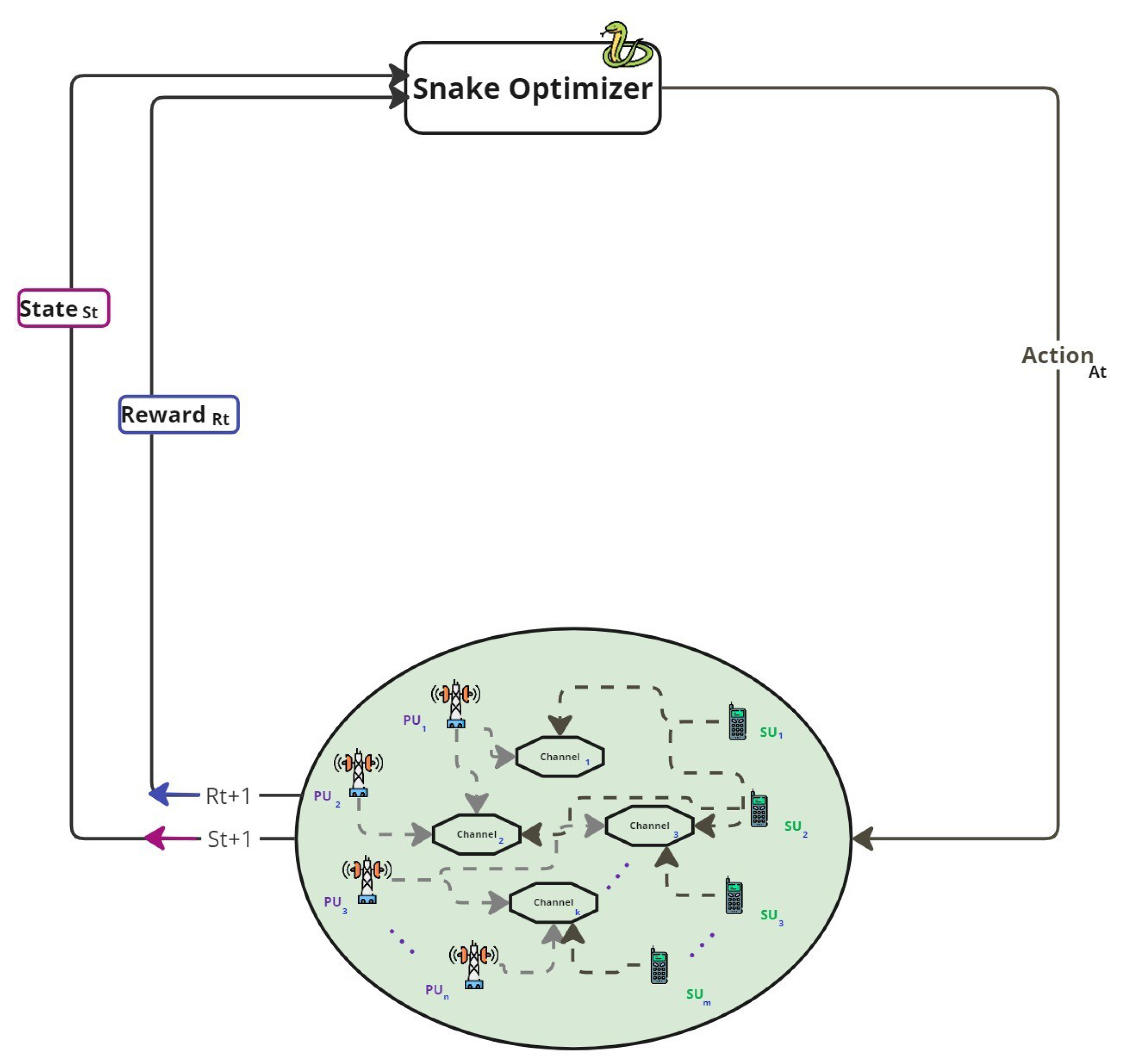
3.2. Proposed Reinforcement Learning with Snake Optimizer

This section presents the RL framework integrated with SO to maximize spectrum utilization in CRN. The essential elements in CRNs are PUs and SUs, where PUs are given priority access to communication channels. The main challenge lies in allocating the idle spectrum to SUs while minimizing interference with PU activity, thereby improving overall network performance.
The SO operates as an RL agent within this environment and interacts dynamically with the CRN to learn an optimal channel allocation policy. At every time step, the agent perceives the current state of the environment S t , which includes the set of active and available SUs over channels P, PU presence information, and interference or collision status. Based on this state, the SO selects an action A t aimed at minimizing interference and maximizing spectral efficiency.
Upon executing the action, the environment transitions to a new state S t + 1 and provides a reward R t that evaluates the impact of the action. The reward depends on reduced collisions, increased spectral efficiency, and overall network throughput. This feedback loop allows the agent to refine its channel allocation strategy iteratively to achieve higher long-term cumulative rewards.
The SO-based RL interaction in the CRN environment is illustrated in Figure 2. This closed-loop system demonstrates how the SO adapts its decisions over time in response to environmental changes, accounting for multiple PUs and SUs operating across available communication channels.
The SO (top of Figure 2) receives the current state S t from the environment, containing details about currently allocated channels and any interference, representing the underlying network conditions. SO uses this state to determine an action A t , representing the number of SUs allocated to each channel to optimize performance. The environment transitions to a new state S t + 1 and computes the corresponding reward R t , which is then returned to SO.
This feedback loop continues as SO iteratively refines its strategy, treating the received rewards as utility for improving future decisions. The primary objective is to achieve flexible and effective channel assignment that maximizes spectral efficiency while avoiding significant impact on co-channel CUs.
The interaction between SO and CRN environments in the RL framework can be mathematically modeled using a set of equations that define state transitions, agent actions, and reward functions. These formulations are critical for understanding how the agent adapts and evolves its allocation strategy over time.
The subsequent state S t + 1 is determined by the current state S t and the action A t executed by the SO, as described below:
S t + 1 = f ( S t , A t ) + ϵ t
Here, f ( S t , A t ) represents the deterministic transition function describing how the system changes in response to an action, and ϵ t accounts for environmental randomness or noise.
The reward R t + 1 received after taking action A t in state S t is defined as follows:
R t + 1 = r ( S t , A t )
To define the reward function more precisely, we express it as a weighted combination of key performance metrics:
R t + 1 = α · SUE t β · CR t + γ · SC t
where SUE t is the spectrum utilization efficiency at time t, CR t is the collision rate, and SC t is the total spectral capacity achieved. The weights α , β , and γ are positive real-valued parameters that control the contribution of each term to the overall reward. For our experiments, we use α = 0.4 , β = 0.3 , and γ = 0.3 , reflecting a balanced trade-off among efficiency, interference avoidance, and throughput. These weights can be adjusted to prioritize different objectives depending on the network conditions or application requirements.
In the context of SO, which merges RL with population-based meta-heuristics, the above reward formulation guides the evolutionary selection process. Since SO does not rely on value approximation but rather on direct fitness evaluation, we reformulate the reward as an explicit fitness function used during optimization:
Fitness t = α · SUE t β · CR t + γ · SC t
This fitness function is effectively equivalent to the reward structure in Equation (3), but is used in the context of solution ranking and selection within the SO algorithm. Readers will encounter related formulas and definitions to this fitness formulation throughout the optimization process in the upcoming sections.
The reward function r ( S t , A t ) evaluates the outcome of taking action A t in state S t . It serves as the primary feedback mechanism guiding the learning process, as the agent aims to maximize the cumulative reward over time by choosing increasingly effective actions.
Ultimately, the agent selects an action A t at each time step based on the current state S t using an optimization strategy defined by the policy:
A t = π ( S t )
The policy π ( S t ) maps from states to actions. It dictates which action the agent should take in a given state to maximize long-term rewards. Together, these equations form the foundation of the RL process, enabling SO to learn and adapt its strategy for optimal channel allocation in CRN. The decision policy π ( S t ) in our framework is implemented in a deterministic manner. It is directly derived from the optimization logic embedded within SO, which selects actions A t based on the current environment state S t and the optimizer’s internal population configuration and fitness evaluations. In contrast to conventional reinforcement learning methods that employ stochastic policies or neural network approximators, our policy is rule-based and deterministic, governed by the heuristic mechanisms of SO. These include the exploration and exploitation strategies influenced by parameters such as the food quantity Q, environmental temperature, and individual fitness levels. This design enables the SO to make interpretable and computationally efficient decisions suitable for real-time spectrum management in dynamic cognitive radio network environments.
To further clarify how SO is embedded within a formal RL framework, we emphasize that our method departs from conventional RL formulations that rely on explicit Q-value updates, value functions, or neural approximators. Instead, SO operates as a meta-heuristic-based RL agent, where the policy is implicitly optimized through population-based exploration and exploitation. The architecture of the agent can be understood in terms of the following components:
  • State representation ( S t ): Each state encapsulates the current occupancy status of channels, presence of PUs, the collision history, and active SUs.
  • Action ( A t ): The action corresponds to a specific allocation of SUs to available channels, selected based on SO’s optimization process.
  • Policy ( π ( S t ) ): Defined implicitly through the heuristic rules of SO algorithm, which evolves solutions over iterations using operations like mating, exploration, and fighting.
  • Reward ( R t ): A scalar value computed based on performance indicators such as spectrum utilization efficiency, number of collisions, and spectral capacity.
  • Learning mechanism: Instead of value iteration or gradient-based learning, SO adjusts its population of candidate solutions based on fitness, without requiring Q-value updates or neural approximators.
It is important to note that the state and action spaces in the proposed RL framework are discrete. Each state S t encodes the availability of channels, current allocation, and observed interference levels, while each action A t corresponds to a specific channel allocation decision for secondary users. The entire interaction process is modeled as a MDP, where SO functions as an agent that selects actions based on the observed state to maximize the expected cumulative reward. This formalism enables the efficient learning of optimal allocation policies under dynamic and uncertain network conditions.

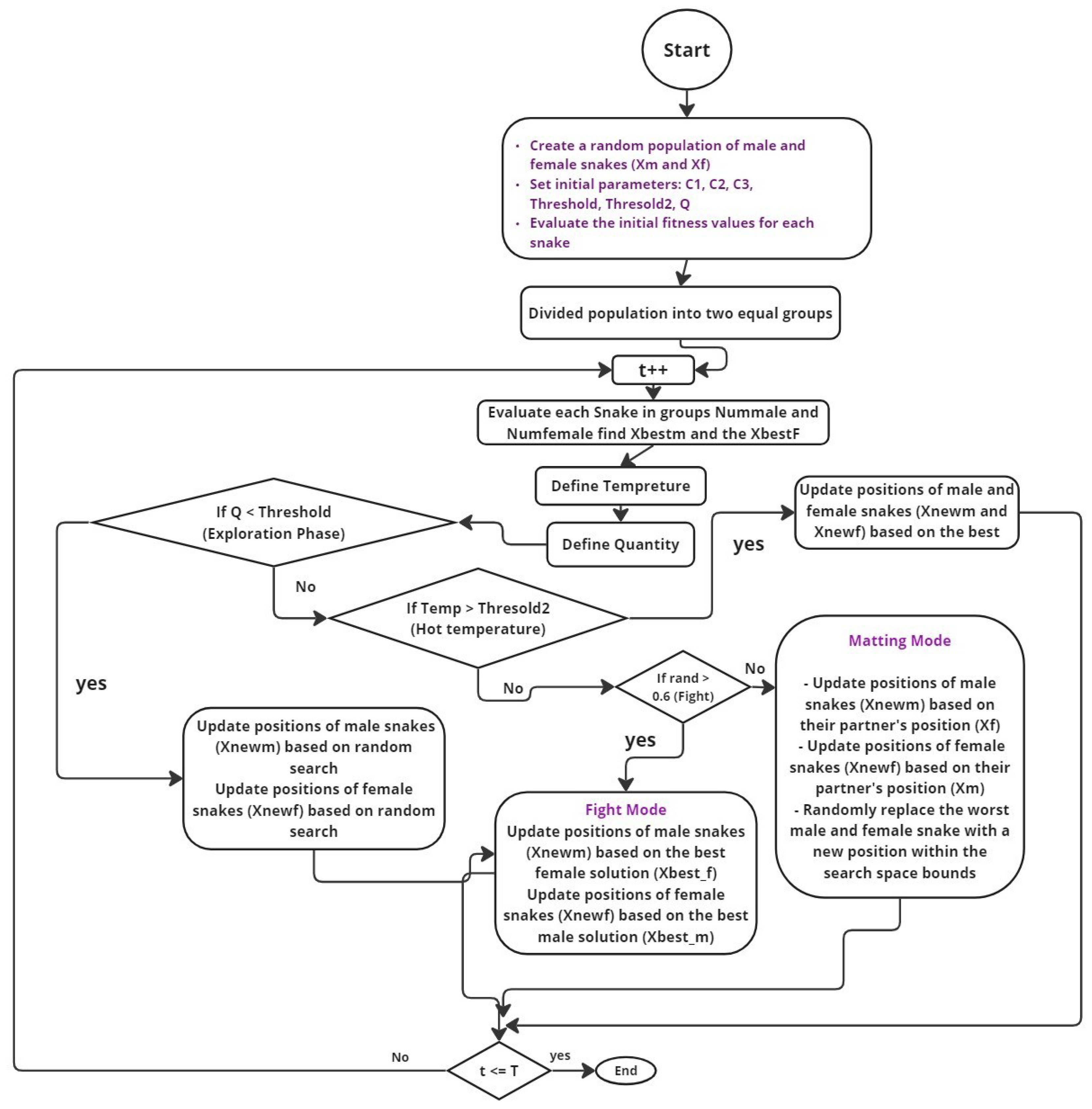
4. Proposed Snake Optimizer

In this section, we present SO with its mathematical model, inspired by the mating behavior of snakes. SO is an optimization algorithm capable of solving complex engineering problems by alternating between exploration and exploitation phases, mimicking the mating and food-searching behaviors of snakes.

4.1. Initialization

SO begins through the initialization of a randomly generated population to initiate the optimization process. Each individual in the population represents a potential solution, and their initial positions are calculated as follows:
X i = X min + r × ( X max X min )
where X i is the position of the ith individual, r [ 0 , 1 ] is a random scalar, and X min and X max are the lower and upper bounds of the search space.

4.2. Population Division

The population is divided into two equal groups: males and females. Their respective counts are determined as follows:
N m N 2
N f = N N m
Here, N is the total population size, N m is the number of males, and N f is the number of females.

4.3. Temperature and Food Quantity Definition

The environmental temperature, influencing the behavior of snakes, is defined as follows:
Temp = exp ( t )
where t is the current iteration, and T is the max number of iterations. The food quantity Q, which determines the shift between exploration and exploitation, is defined by the following:
Q = c 1 × exp t T T
where c 1 is a constant, typically set to 0.5.

4.4. Exploration Phase: No Food Available

To clarify the dimensions used in the update equations, we define the matrices A m and A f as the position sets of male and female individuals, respectively. Let the total population size be N and the dimensionality of the problem be D (equal to the number of SUs multiplied by the number of available channels). Then, A m R N m × D and A f R N f × D , where N m = N / 2 and N f = N N m . Each row of these matrices corresponds to the D-dimensional position vector of an individual in the population. When Q < 0.25 , snakes perform exploration by randomly searching the space. Position updates for individuals are as follows:
For males:
X i , m ( t + 1 ) = X rand , m ( t ) ± c 2 · A m · ( X max X min ) · rand + X min
For females:
X i , f ( t + 1 ) = X rand , f ( t ) ± c 2 · A f · ( X max X min ) · rand + X min
where X rand , m ( t ) , X rand , f ( t ) are positions of randomly selected males and females; A m and A f are their respective abilities to search; and c 2 is a constant (typically 0.05).
Abilities are computed by the following:
A m = exp f rand , m f i , m
A f = exp f rand , f f i , f
where f rand , m and f rand , f are fitness values of randomly selected individuals, and f i , m and f i , f refer to the ith male and female individuals.

4.5. Exploitation Phase (Food Available)

When food quantity Q exceeds the threshold (Threshold = 0.25), snakes enter the exploitation phase. If temperature is high (Temp > 0.6), individuals move directly toward food:
X i , j ( t + 1 ) = X food ± c 3 · Temp · rand · ( X food X i , j ( t ) )
where X i , j ( t ) is the current position of the ith individual (male or female), X food is the position of the best individual (food), and c 3 is a constant (typically 2).
When temperature is low (Temp < 0.6), snakes may engage in either the fight or mating mode.
Fight Mode:
X i , m ( t + 1 ) = X i , m ( t ) + c 3 · F M · rand · ( Q · X best , f X i , m ( t ) )
X i , f ( t + 1 ) = X i , f ( t + 1 ) + c 3 · F F · rand · ( Q · X best , m X i , f ( t ) )
where F M and F F are the fighting abilities:
F M = exp f best , f f i , m
F F = exp f best , m f i , f
Mating Mode:
X i , m ( t + 1 ) = X i , m ( t ) + c 3 · M m · rand · ( Q · X i , f ( t ) X i , m ( t ) )
X i , f ( t + 1 ) = X i , f ( t ) + c 3 · M f · rand · ( Q · X i , m ( t ) X i , f ( t ) )
with mating abilities:
M m = exp f i , f f i , m
M f = exp f i , m f i , f
If mating results in successful reproduction (egg hatching), the worst male and female individuals are replaced:
X worst , m = X min + rand · ( X max X min )
X worst , f = X min + rand · ( X max X min )
The termination of the algorithm occurs when the maximum number of iterations is reached or when a satisfactory solution is found. The algorithm then returns the best solution discovered during the optimization process. Figure 3 illustrates the mating behavior of snakes, which serves as the inspiration for the Snake Optimization algorithm. In nature, snake mating typically occurs in cold environments, such as late spring or early summer, where temperature and food availability are key factors. Figure 3 likely depicts two main phases: the exploration phase and the exploitation phase, both of which are critical in SO. During the exploration phase, snakes search for food when it is scarce. If food is available, and the temperature is appropriate, the snakes enter the exploitation phase, where they focus on mating behavior. This phase can further be divided into “fight mode,” where males compete for the best females, and “mating mode,” where successful mating occurs. Figure 3 emphasizes the dynamic nature of snake behavior, which the SO algorithm mimics to solve optimization problems by balancing exploration and exploitation. Figure 3 is designed to offer a conceptual overview that integrates two perspectives: (i) the biological inspiration drawn from snake mating and foraging behavior, which forms the basis of SO’s meta-heuristic design; and (ii) the optimizer’s operational role within an RL framework applied to CRNs. While the visual combines elements from both domains, it serves to illustrate the analogy between natural behavior and algorithmic decision-making processes. The goal is to provide intuitive understanding rather than to present a strict architectural separation.

4.6. Pseudocode and Operational Flow

Algorithm 1 outlines the complete workflow of SO, including initialization, behavioral logic (exploration and exploitation), mating mechanisms, and termination criteria. This section complements the previous one by translating the mathematical expressions into a procedural representation. To address clarity and completeness, we consolidate the theoretical formulation and implementation of SO algorithm through: (i) its behavioral equations (Equations (6)–(25)), (ii) a comprehensive pseudocode representation (Algorithm 1), and (iii) detailed parameter explanations (Table 2). These components collectively allow readers to understand, implement, and evaluate the algorithm effectively.
Algorithm 1 Snake Optimizer in reinforcement learning framework
1:Initialize Problem Parameters:
2:    - Dimension of the problem ( D i m )
3:    - Upper Bound ( U B ) and Lower Bound ( L B ) of the search space
4:    - Population size ( P o p _ S i z e ), Maximum Iterations ( M a x _ I t e r )
5:    - Current Iteration ( C u r r _ I t e r ) set to 0
6:Initialize Population Randomly:
7:    - Generate initial positions for each individual within the bounds
8:Divide Population into Two Equal Groups:
9:    Divide population into N m (males) and N f (females):
10:      N m N 2
11:      N f = N N m
12:while  C u r r _ I t e r M a x _ I t e r  do
13:    Evaluate Fitness of Each Individual
14:    Find Best Male ( f b e s t , m ) and Best Female ( f b e s t , f )
15:    Define Environmental Temperature:
16:        T e m p = exp ( C u r r _ I t e r M a x _ I t e r )
17:    Define Food Quantity:
18:        Q = c 1 × exp C u r r _ I t e r M a x _ I t e r M a x _ I t e r
19:    if  Q < 0.25  then
20:        Perform Exploration Phase:
21:            - Randomly update positions of males and females
22:    else if  Q > 0.6  then
23:        Perform Exploitation Phase:
24:        if  T e m p > 0.6  then▹ hot
25:           - Move towards best-known food position
26:        else▹ cold
27:           - Enter Fight Mode or Mating Mode
28:           Fight Mode: Compete for best individuals
29:           Mating Mode: Mate and update positions
30:        end if
31:    end if
32:    if Mating Occurs then
33:        - Hatch eggs and replace worst individuals
34:    end if
35:    Update Iteration: C u r r _ I t e r C u r r _ I t e r + 1
36:end while
37:Termination:
38:    - If max iterations or other criteria met, stop
39:return Best Solution Found
Table 2 provides an in-depth look at the critical parameters employed in SO algorithm as described in the code. Each parameter is crucial to the functioning of the optimization process, and Table 2 offers a clear understanding of how these parameters are set or initialized.
The number of SUs is a scenario-dependent parameter that defines the total number of SUs in the cognitive radio network. Similarly, the number of PUs also varies based on the scenario, influencing how the network resources are allocated between primary and secondary users. The number of bands available for communication is another scenario-dependent parameter that sets the spectrum space that secondary users can access. The iteration counts represent different maximum iteration limits, specifically 30, 50, and 100, tested during the optimization process. These iteration limits allow the algorithm to be evaluated under varying conditions, helping to identify the most effective strategy. The number of runs, set to 10, indicates that the optimization process is repeated multiple times for each scenario, ensuring that the results are averaged over these runs to provide a more robust assessment of SO’s performance.
Max iterations refer to the maximum number of iterations permitted for each simulation run of SO. This value is dynamically assigned from the iteration counts being tested. The population size, although not explicitly defined in the provided code, plays a significant role in determining the diversity of solutions generated by the optimizer. The best fitness value is initially set to negative infinity, indicating that the optimizer will accept any improvement during the early stages of the process. Convergence time is initialized to the maximum number of iterations, serving as a benchmark to measure how quickly the optimizer can find a near-optimal solution.
Table 2 also lists constants used during the exploration and exploitation phases, such as the exploration constant and the exploitation constant. These constants control the balance between searching for new solutions and refining existing ones. Environmental factors like temperature and food quantity are modeled mathematically, with temperature influencing the behavior of the optimizer based on the iteration count, and food quantity guiding the transition between exploration and exploitation phases.
Fitness history is initialized to a NaN array, ready to store the fitness values of solutions across iterations. Spectral capacity is assumed to have a maximum of 1 bps/Hz per band, serving as a benchmark for evaluating the network’s performance. Finally, the collision rate and utilization efficiency are calculated based on the final allocation of bands to secondary users, providing key metrics for assessing the effectiveness of SO. Compared to traditional meta-heuristics such as PSO, GA, or ACO, SO introduces biologically inspired modes (e.g., fight and mating) that enable it to adaptively balance exploration and exploitation based on environmental cues (e.g., food availability, temperature). Unlike velocity-driven updates (in PSO) or crossover/mutation operators (in GA), SO employs a behavioral mechanism that is both dynamic and context-aware.

5. Results and Discussion

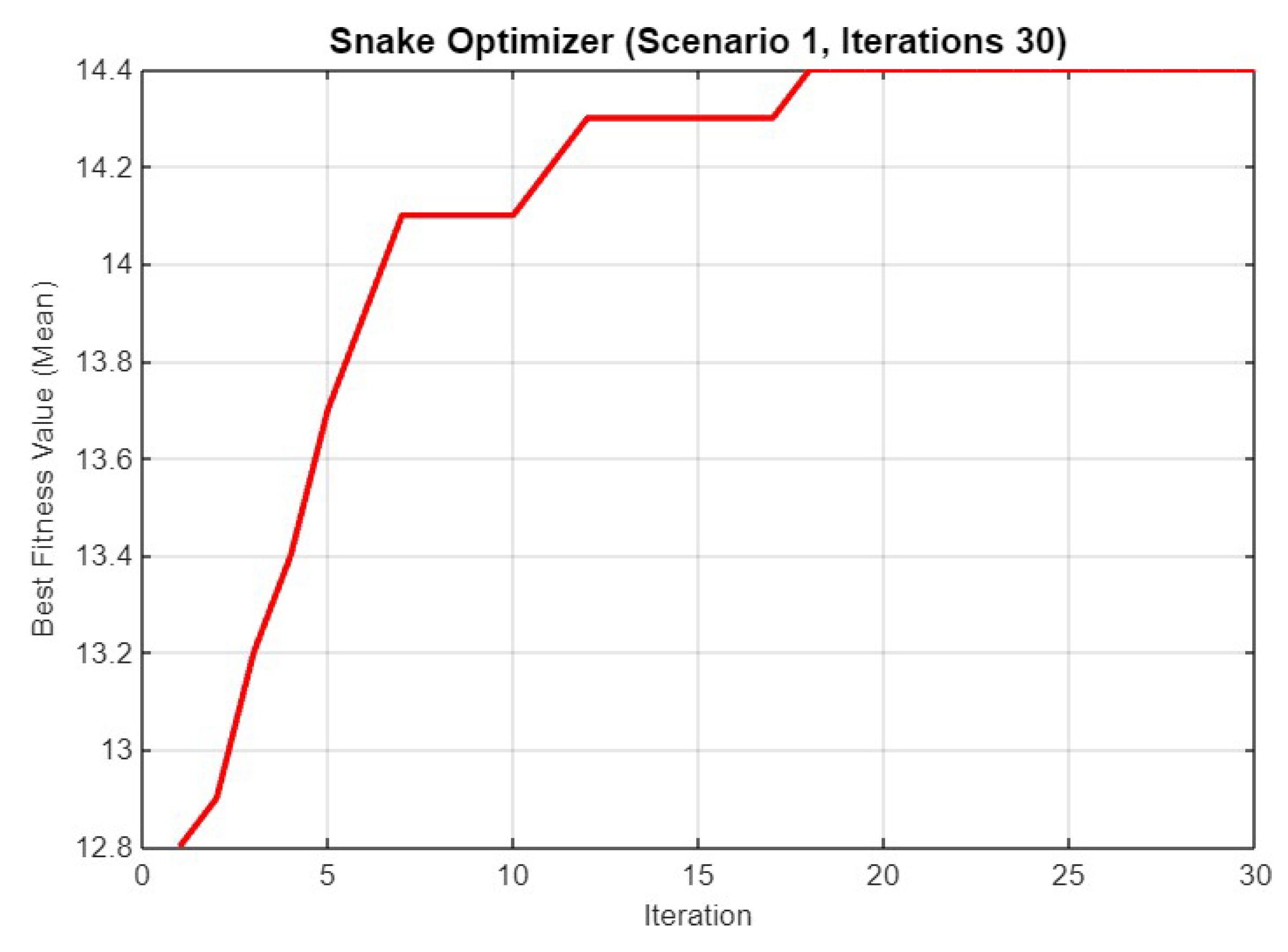
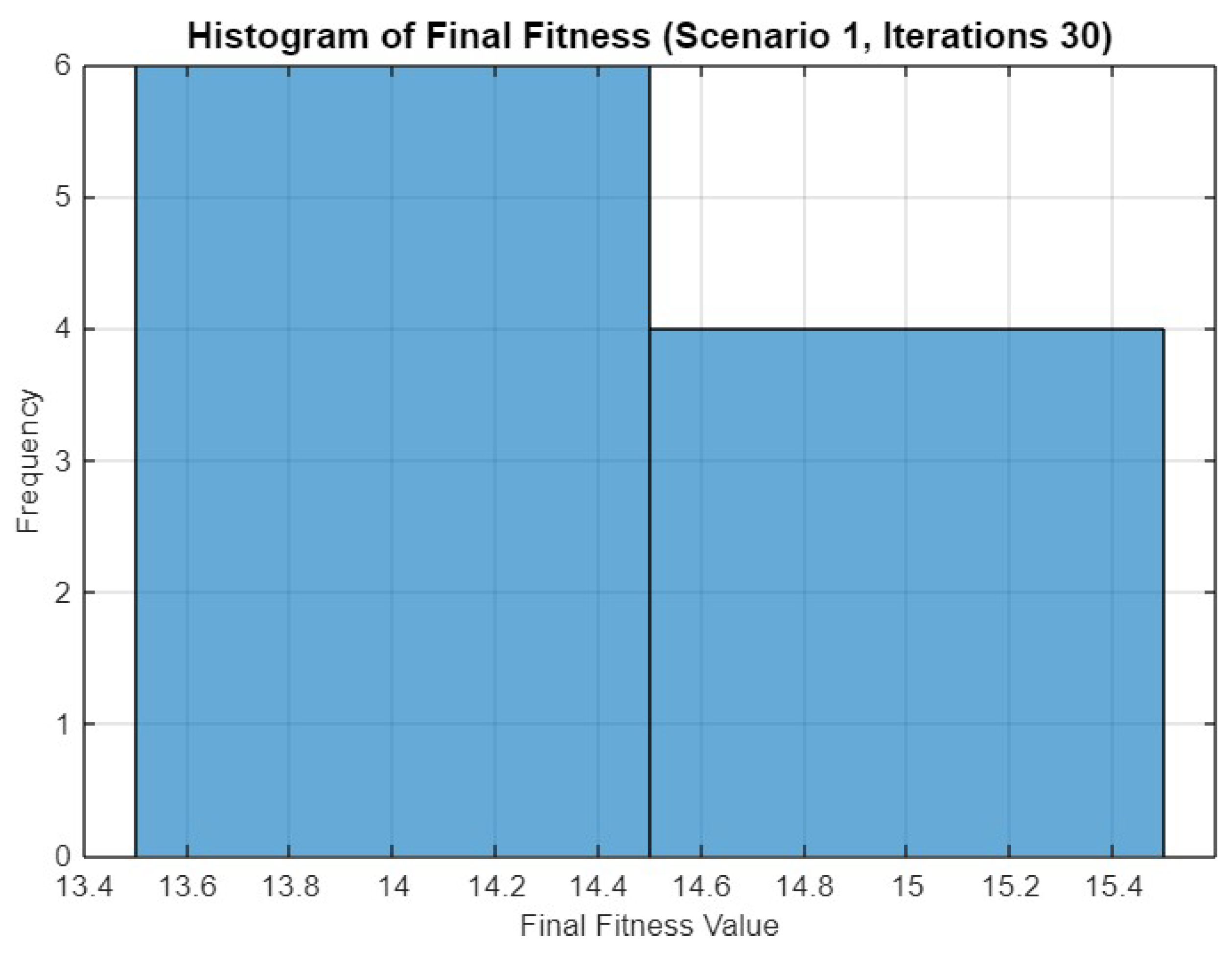
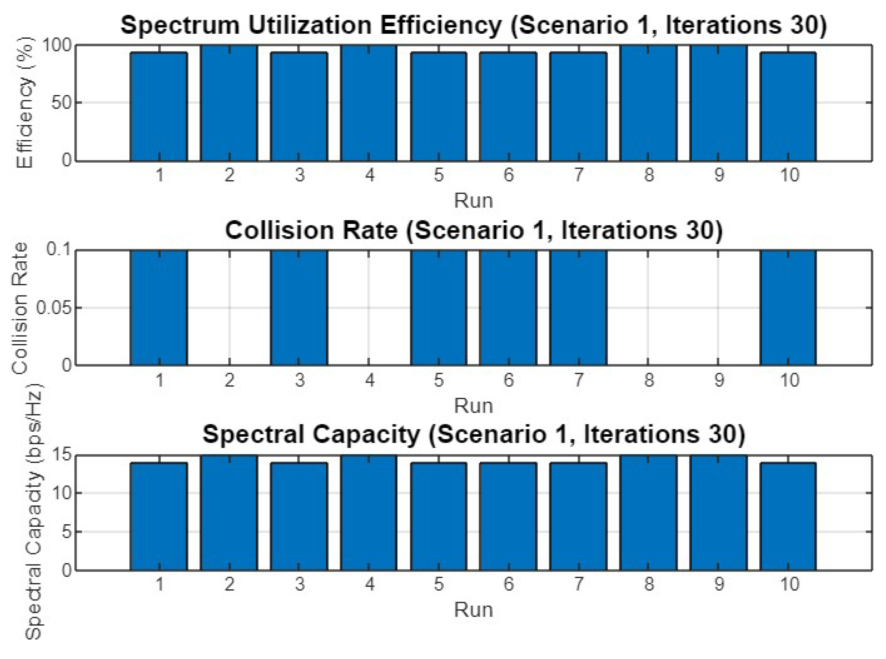
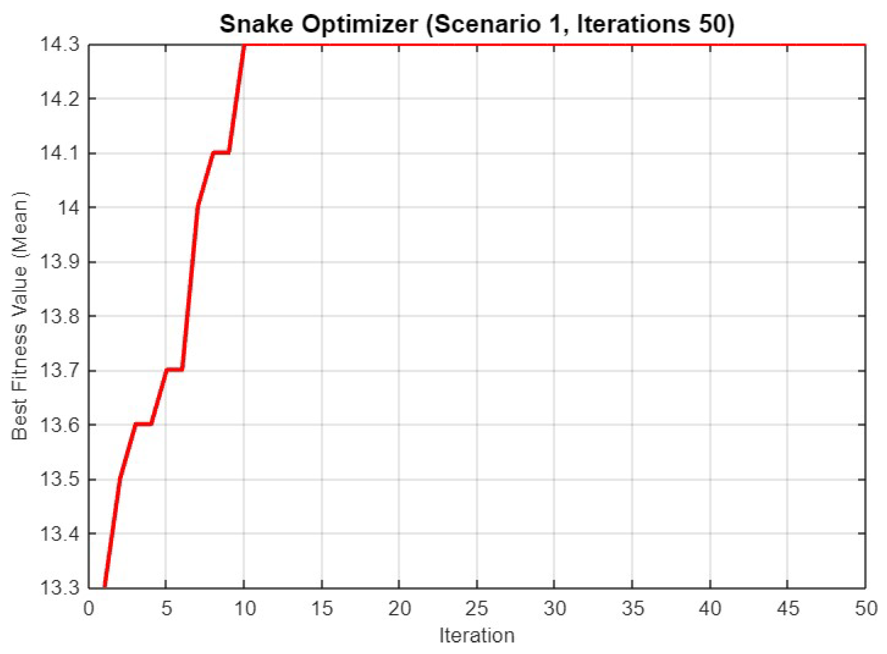
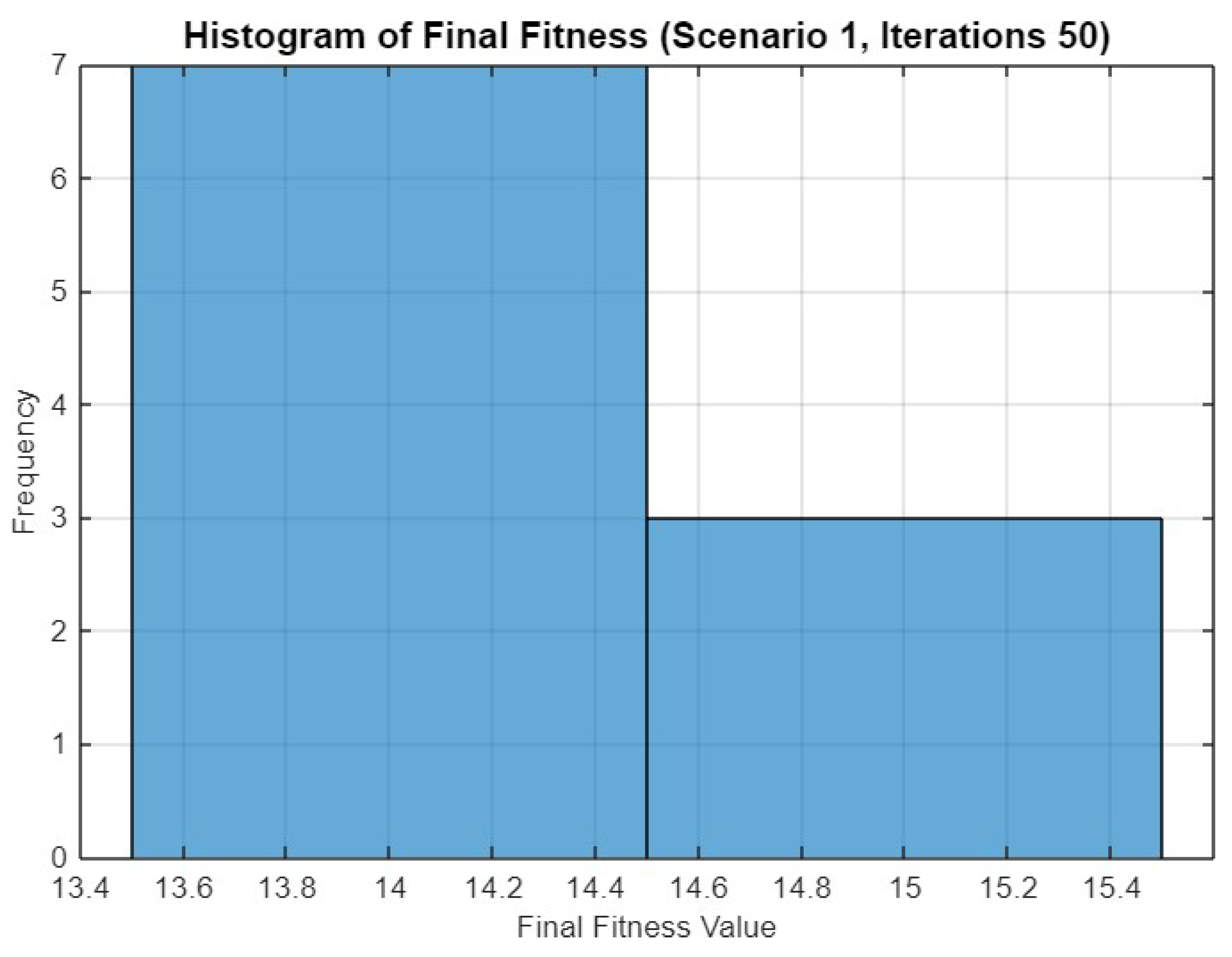
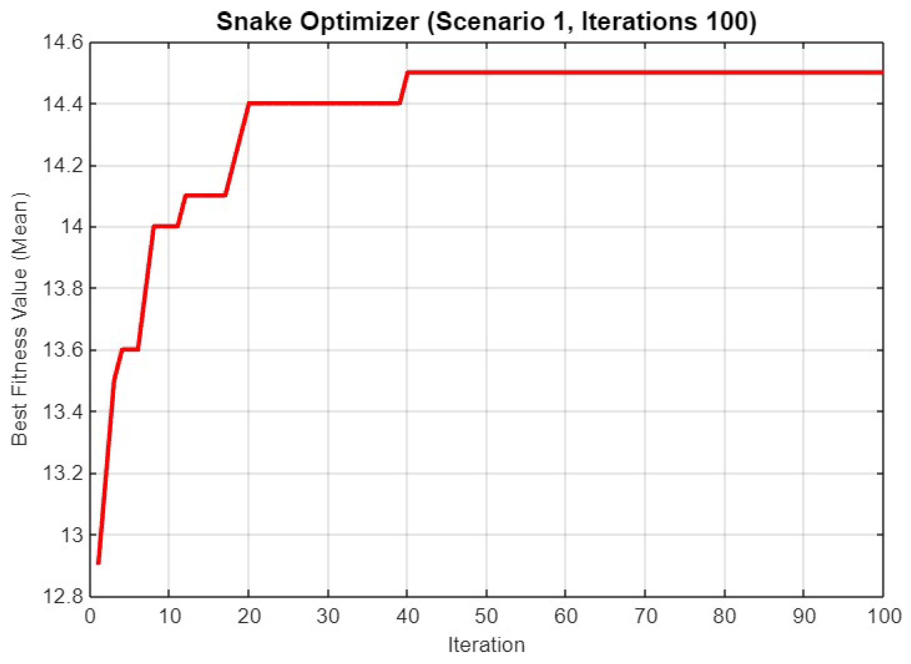
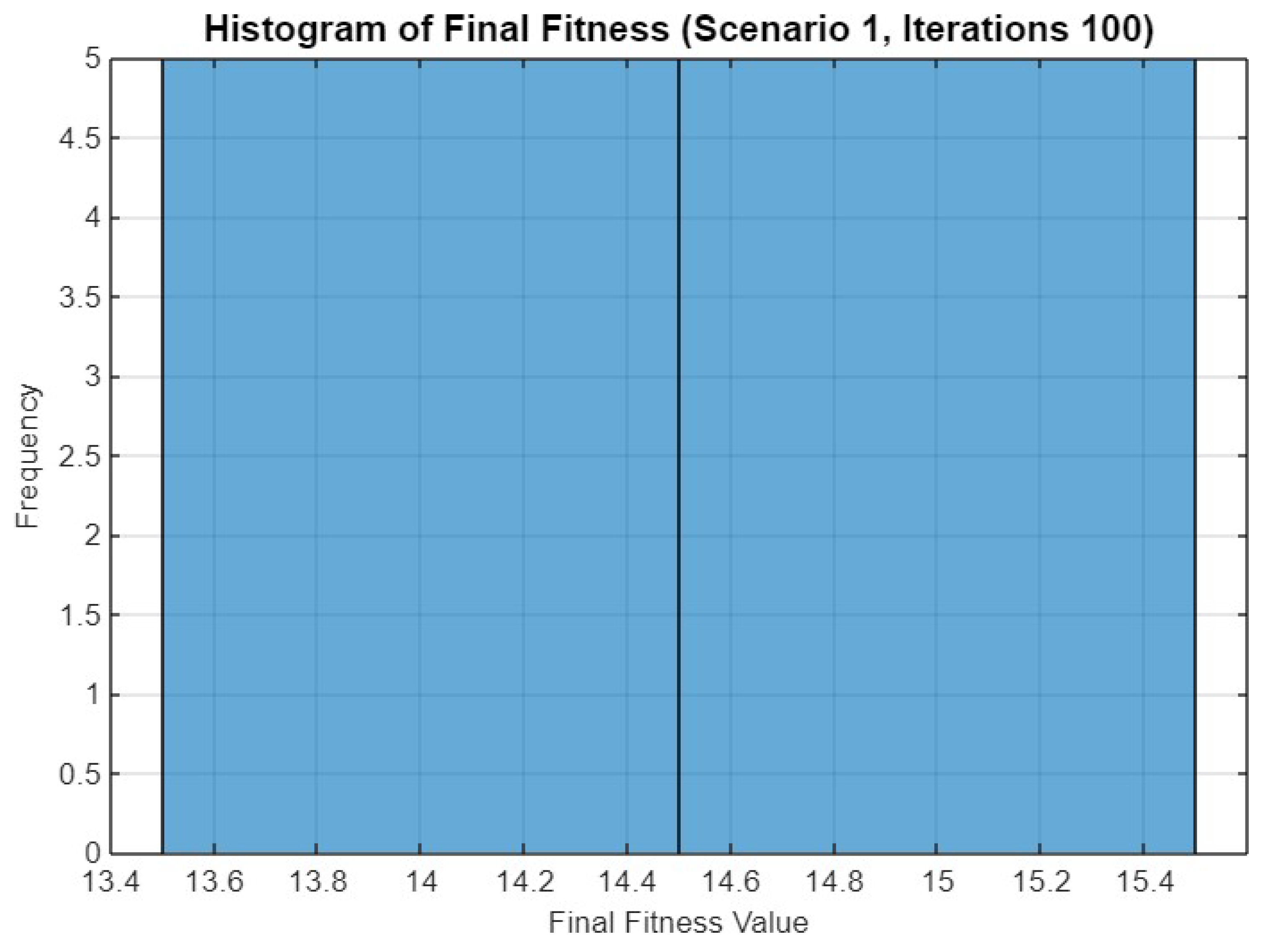
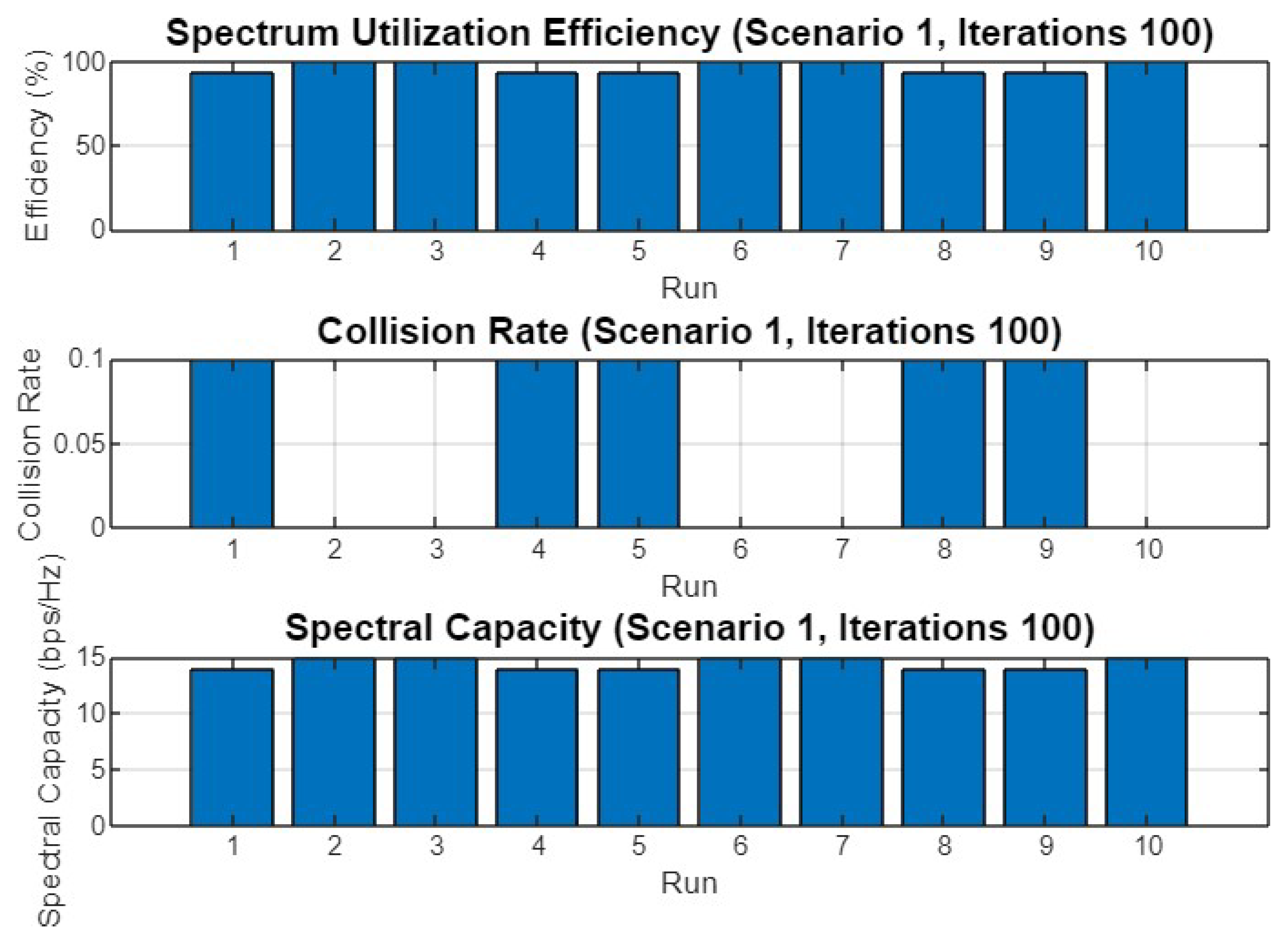
5.1. Experiment Result for First Scenario

The experiment results for the first scenario of SO are depicted through Figure 4, Figure 5, Figure 6, Figure 7, Figure 8, Figure 9, Figure 10, Figure 11 and Figure 12, showing various aspects of the optimization process across different iteration counts.
Figure 4 illustrates the mean best fitness value over 30 iterations. The curve shows a rapid increase in fitness during the initial iterations, reaching a plateau around the 10th iteration. The final mean fitness value stabilizes at approximately 14.3, indicating that the optimizer quickly converges to a near-optimal solution.
Figure 5 presents a histogram of the final fitness values obtained after 30 iterations. The histogram reveals a distribution where most runs resulted in a fitness value close to 14.4, with a few outliers reaching up to 15.4. This suggests that while the optimizer generally converges to similar solutions, there is some variability in the outcomes.
Figure 6 shows the performance metrics across different runs in the first scenario with 30 iterations. The spectrum utilization efficiency is consistently high across all runs, close to 100%. The collision rate remains low, indicating effective avoidance of interference among secondary users. Spectral capacity fluctuates slightly across runs but generally stays within a similar range, demonstrating the optimizer’s ability to maintain efficient use of available channels.
Figure 7 displays the mean best fitness value over 50 iterations. The fitness value increases more gradually compared to the 30-iteration case, eventually stabilizing at around 14.3, similar to the previous result. This suggests that additional iterations do not significantly improve the solution’s quality beyond a certain point.
Figure 8’s histogram of final fitness values for 50 iterations shows a similar distribution to Figure 5, with most values clustering around 14.4 and a few reaching higher fitness levels. This consistency across different iteration counts indicates the robustness of the SO.
In Figure 9, the performance metrics for 50 iterations are plotted. The results are consistent with those observed in Figure 6, with high spectrum utilization efficiency, low collision rates, and stable spectral capacity across all runs. This further supports the optimizer’s effectiveness across different settings.
Figure 10 depicts the mean best fitness value over 100 iterations. The fitness value again follows a steep rise in the early iterations, leveling off around the 30th iteration and stabilizing at approximately 14.5. The slight increase in the final fitness value compared to the shorter iteration counts suggests that more iterations can lead to marginal improvements.
Figure 11 shows the histogram of final fitness values after 100 iterations. The distribution is narrower compared to the previous histograms, with most runs resulting in a fitness value of around 14.4 to 14.6. This indicates a higher degree of convergence consistency when more iterations are allowed.
Finally, Figure 12 presents the performance metrics for 100 iterations. The spectrum utilization efficiency remains high, the collision rate is low, and the spectral capacity is consistent across all runs. These results confirm the stability and reliability of SO in maintaining optimal performance even as the number of iterations increases.

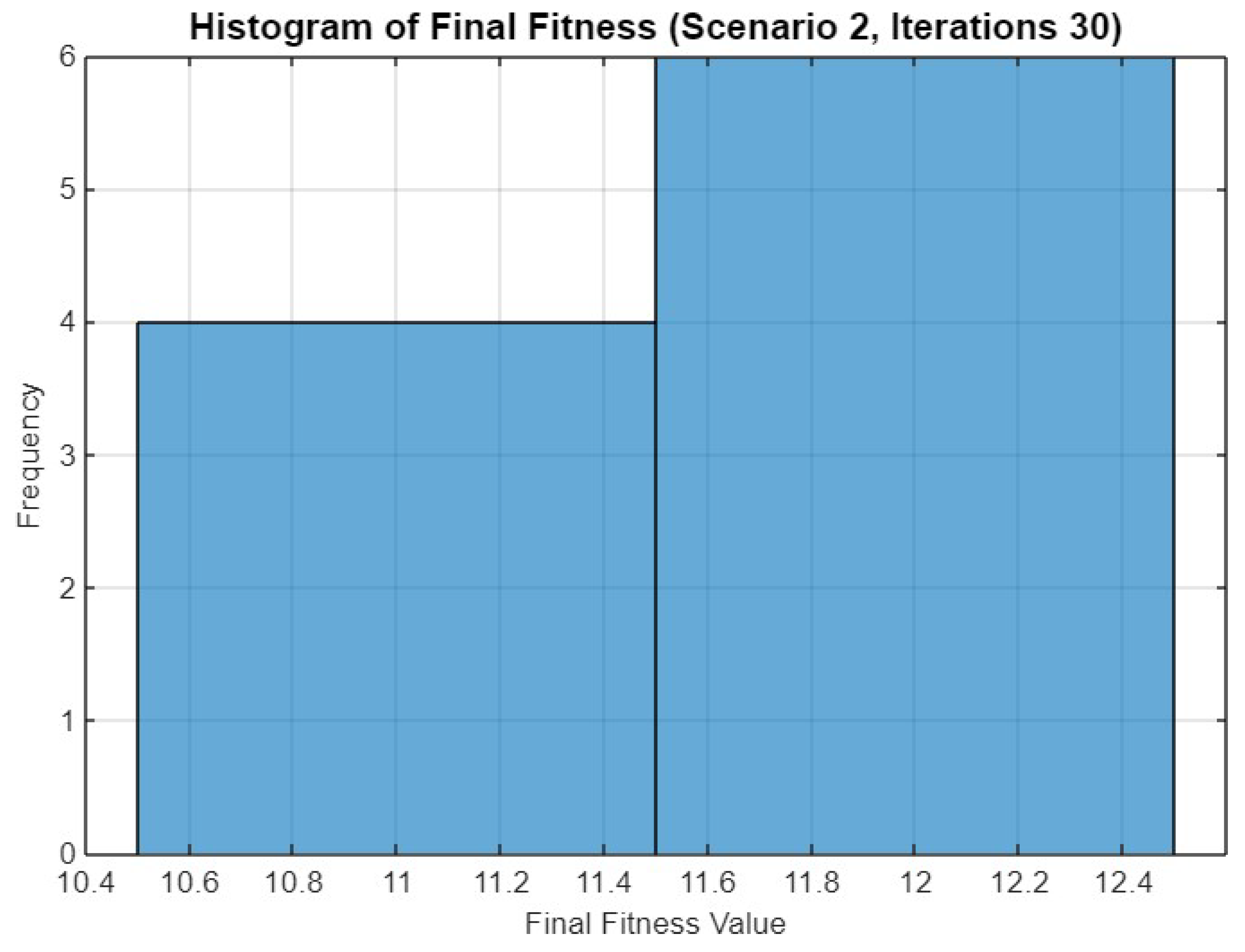
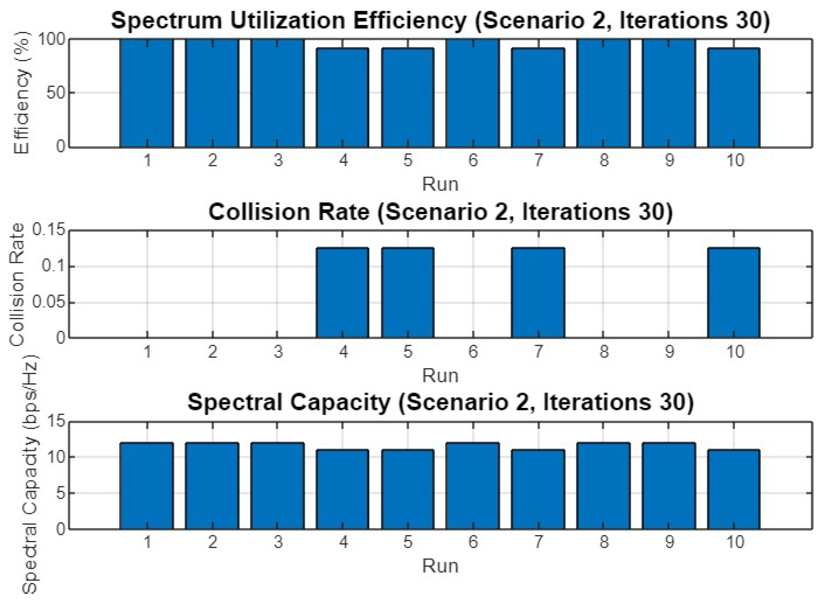
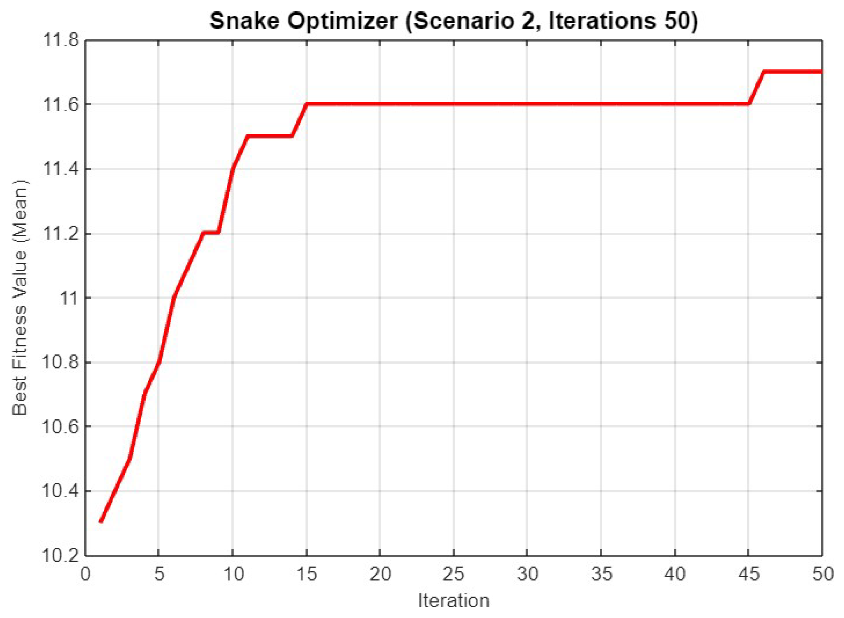
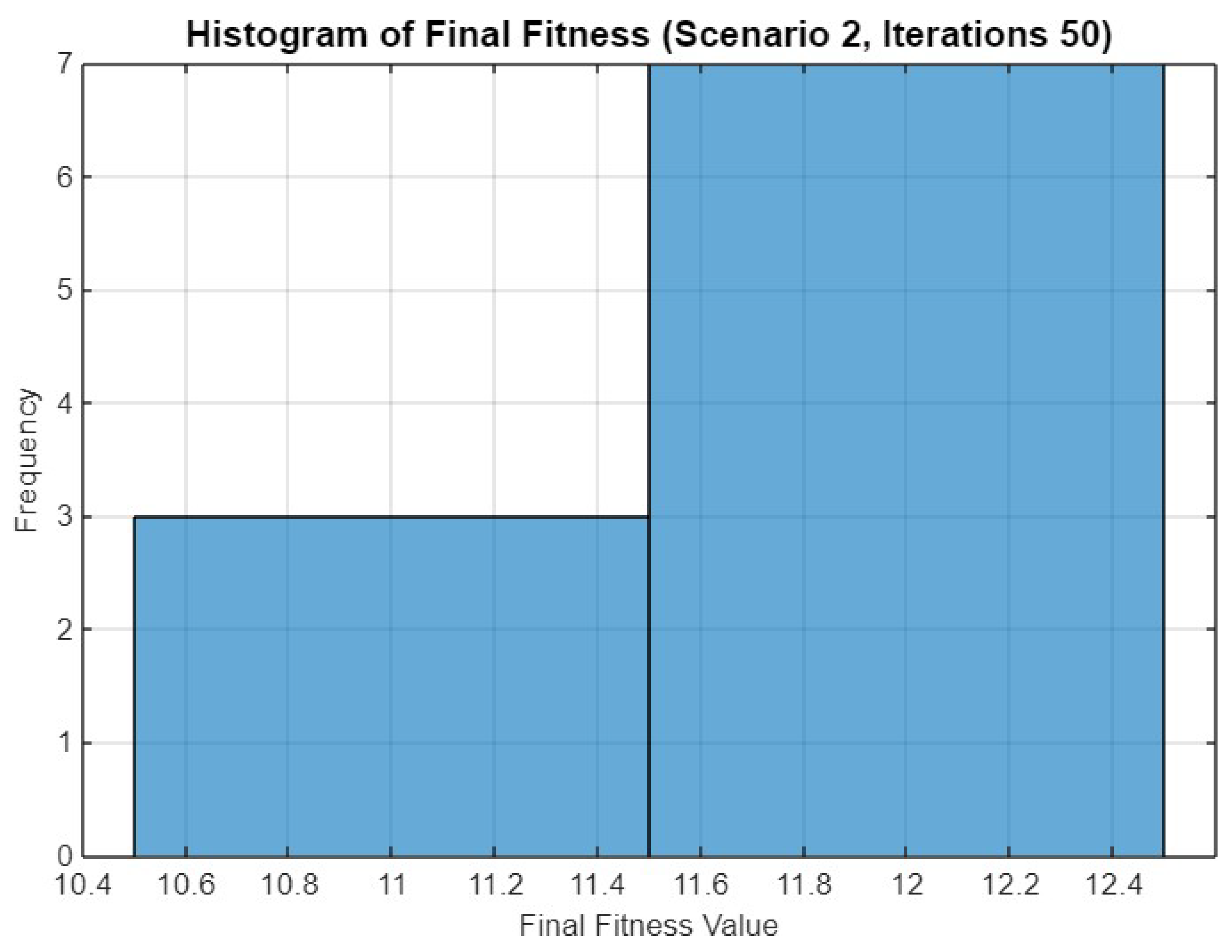
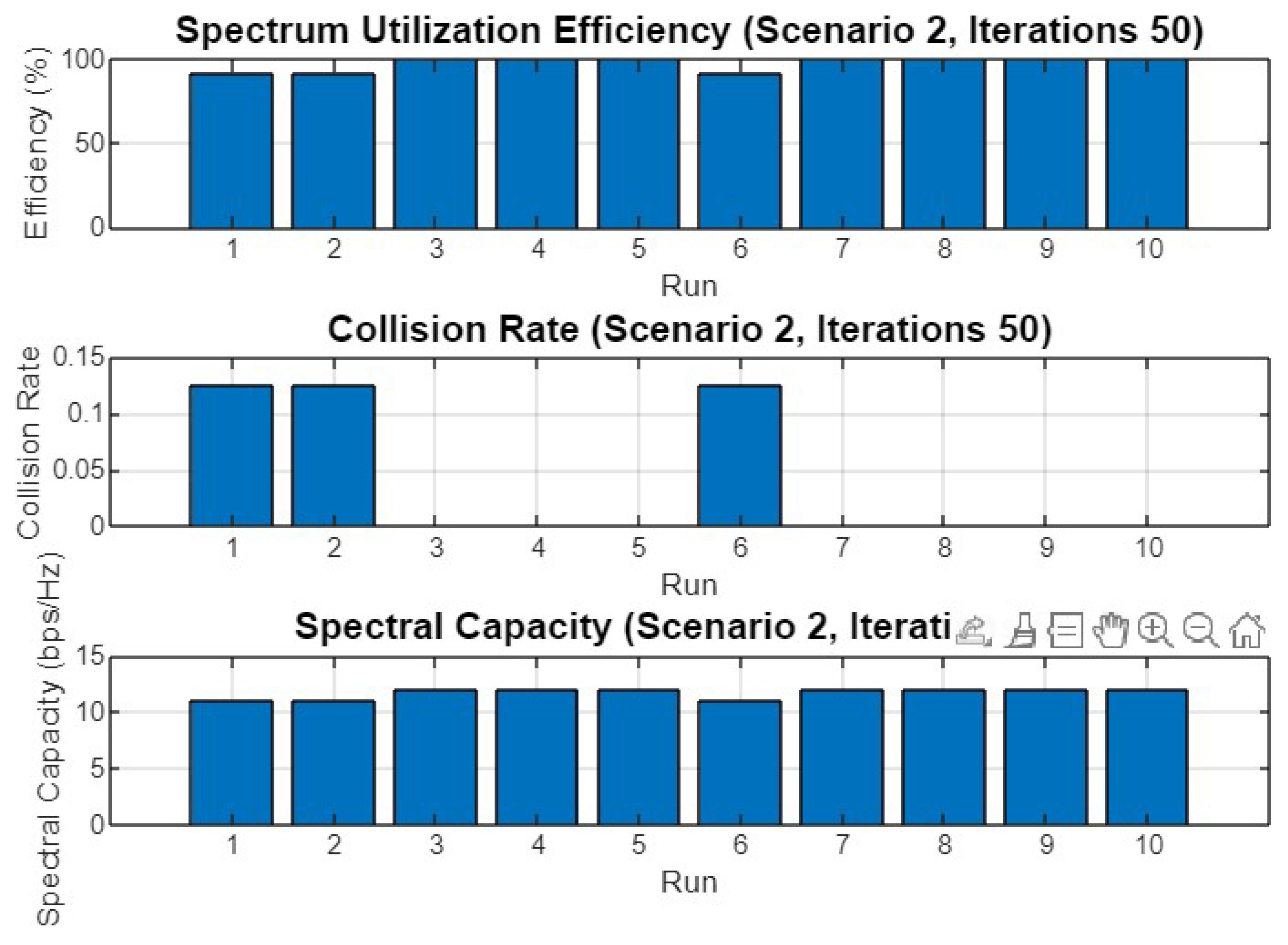
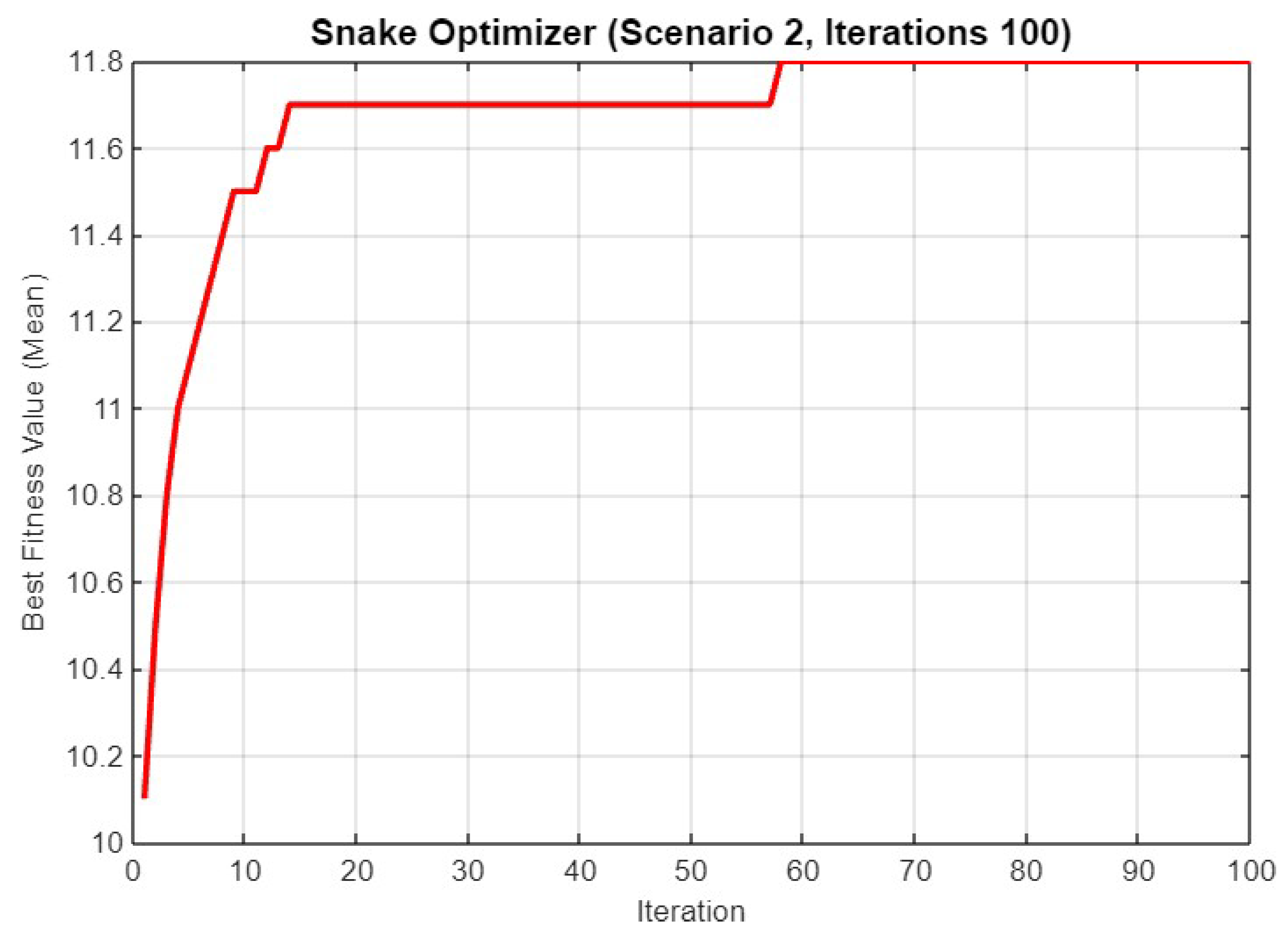
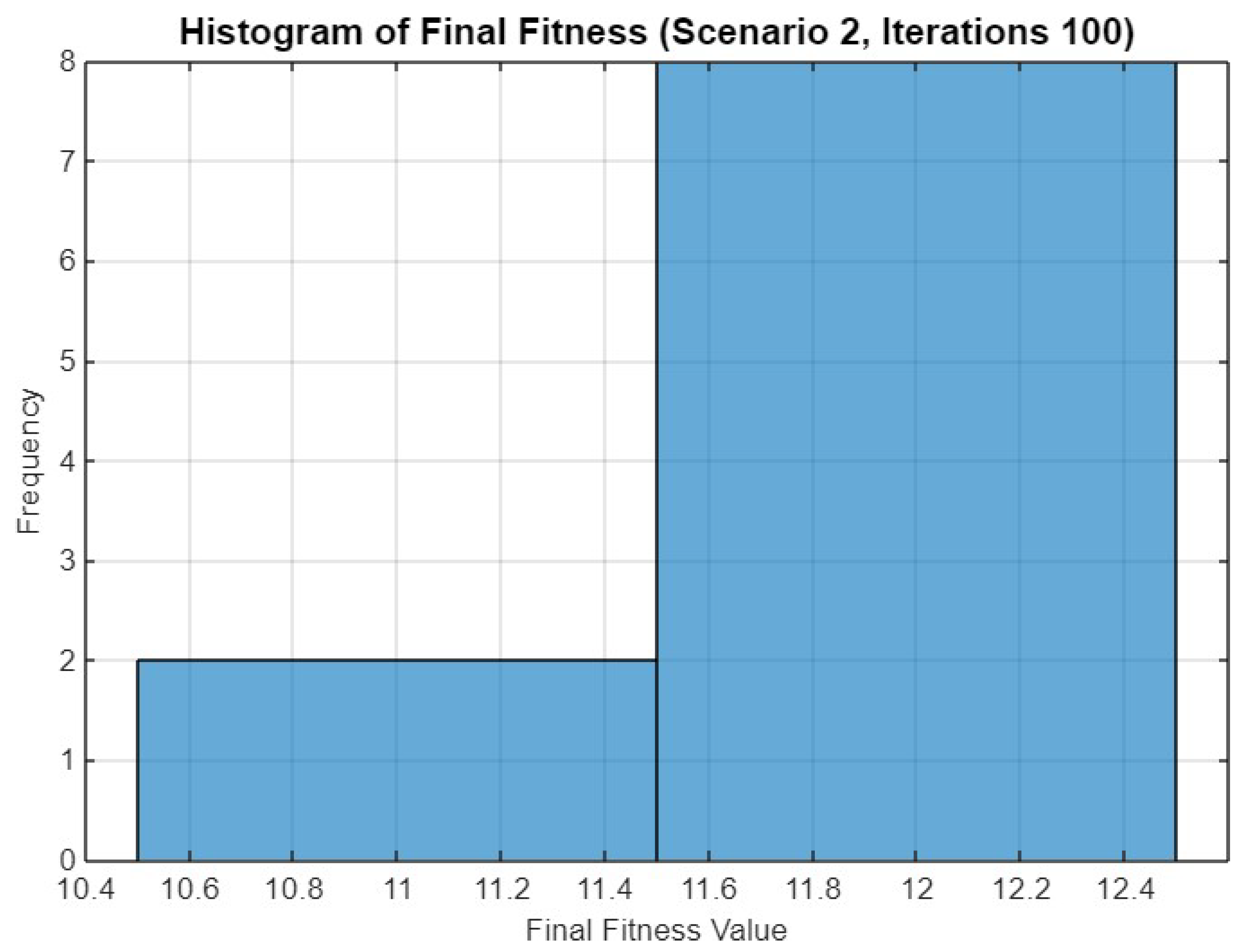
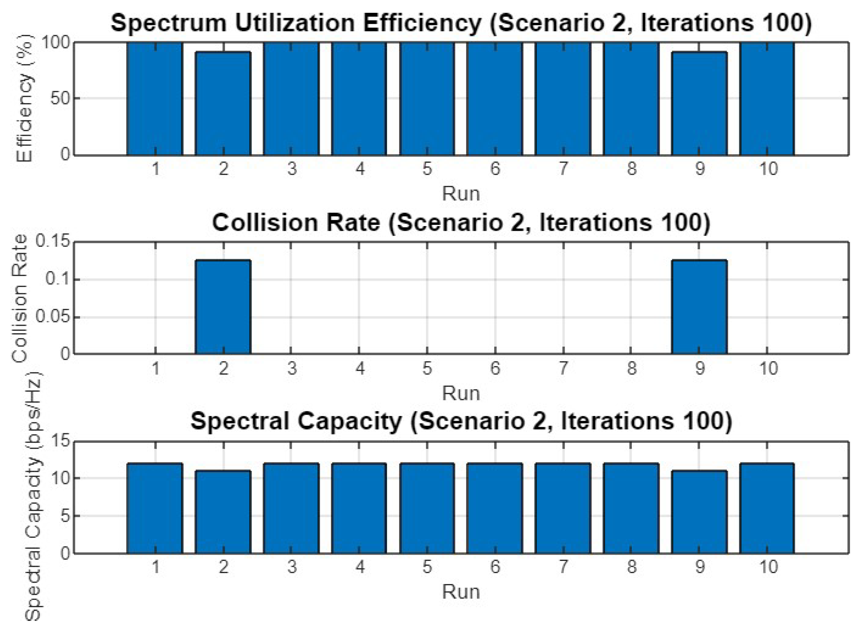
5.2. Experiment Result for Second Scenario

Figure 13 depicts the progression of the best fitness value (mean) for Scenario 2 across 30 iterations. The fitness value starts at approximately 10.6 and gradually increases, showing consistent improvement as the iterations proceed. The optimizer shows significant jumps in fitness around the 10th and 15th iterations, finally stabilizing at a peak fitness value of around 11.6, indicating the convergence of SO towards an optimal solution within this iteration count.
Figure 14 presents a histogram of the final fitness values achieved in Scenario 2 after 30 iterations. The histogram reveals that the majority of the optimization runs yield a fitness value concentrated between 11.4 and 12.4. A smaller cluster of runs shows a lower fitness range between 10.6 and 11.4. This distribution suggests that while the optimizer consistently reaches high fitness values, there is some variability in the final outcomes across different runs.
Figure 15 displays the performance metrics across 10 different runs for Scenario 2 after 30 iterations. The spectrum utilization efficiency is notably high, with most runs achieving close to 100% efficiency. However, there are slight variations, particularly in the collision rate, where run 7 experiences a peak of 0.15, indicating occasional conflicts in channel allocation. Despite this, the spectral capacity remains steady across all runs, suggesting that the optimization process maintains a stable and effective use of the available spectrum.
Figure 16 illustrates the best fitness value (mean) for Scenario 2 over 50 iterations. The fitness value starts at approximately 10.2 and rises sharply within the first 15 iterations to around 11.6, where it remains consistent for the rest of the iterations. This early plateau suggests that SO efficiently finds a near-optimal solution within the first third of the iteration count, maintaining this fitness level thereafter.
Figure 17 provides a histogram of the final fitness values after 50 iterations in Scenario 2. The histogram shows a significant clustering of values between 11.6 and 12.4, with fewer runs achieving fitness values between 10.4 and 11.4. This distribution indicates a successful convergence of most runs towards higher fitness levels, reflecting the optimizer’s effectiveness in this scenario.
Figure 18 shows the performance metrics across 10 runs for Scenario 2 after 50 iterations. The spectrum utilization efficiency remains consistently high across all runs, indicating the optimizer’s effectiveness in managing spectrum resources. The collision rate is low, with a notable exception in run 6 where a slight increase is observed. The spectral capacity remains stable across all runs, indicating that the optimization process consistently maximizes the available spectral resources.
Figure 19 depicts the best fitness value (mean) for Scenario 2 over 100 iterations. The fitness value starts at around 10.2 and increases sharply to 11.8 within the first 20 iterations. This value remains stable for the rest of the iterations, indicating that SO quickly converges to an optimal solution, maintaining this level of performance for the majority of the iteration count.
Figure 20 presents a histogram of the final fitness values for Scenario 2 after 100 iterations. The histogram shows that the final fitness values are heavily clustered between 11.6 and 12.4, with a small number of runs achieving fitness values between 10.4 and 11.4. This distribution reflects a strong convergence towards higher fitness levels, showcasing the optimizer’s robustness in this extended iteration scenario.
Figure 21 displays the performance metrics for Scenario 2 after 100 iterations across 10 different runs. The spectrum utilization efficiency is high across all runs, with slight variations but generally consistent performance. The collision rate is low, with only run 2 showing a minor spike. The spectral capacity remains stable across all runs, reflecting the optimizer’s ability to maintain an effective use of the available spectrum even over an extended number of iterations.

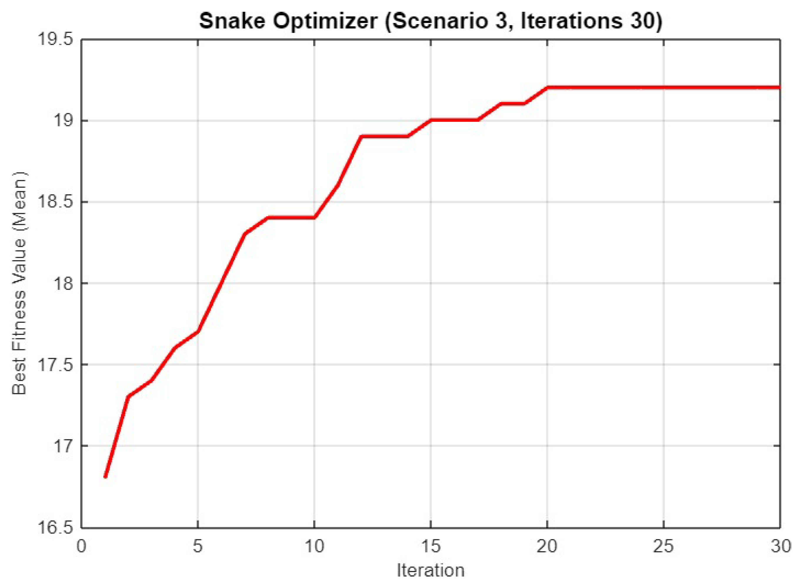
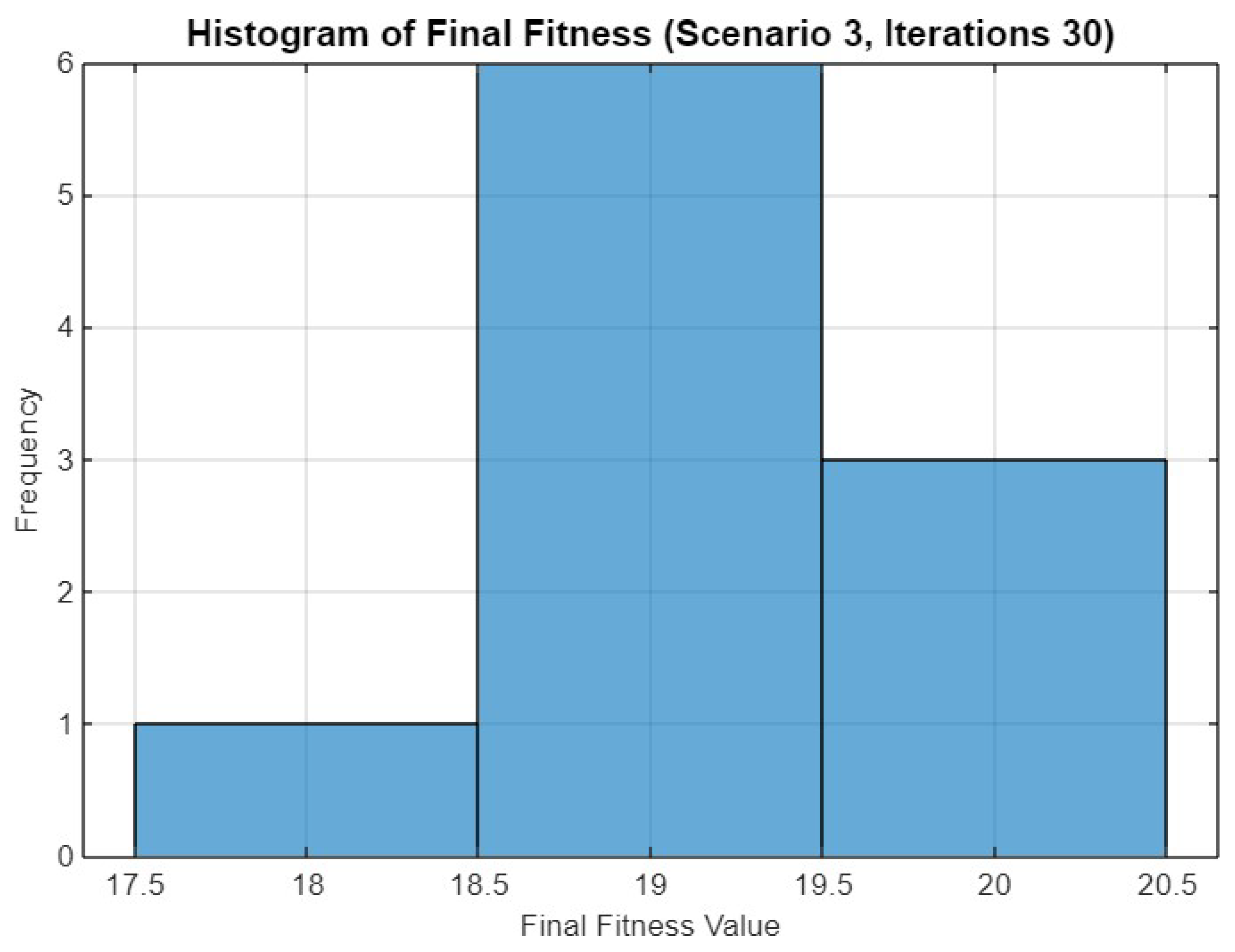
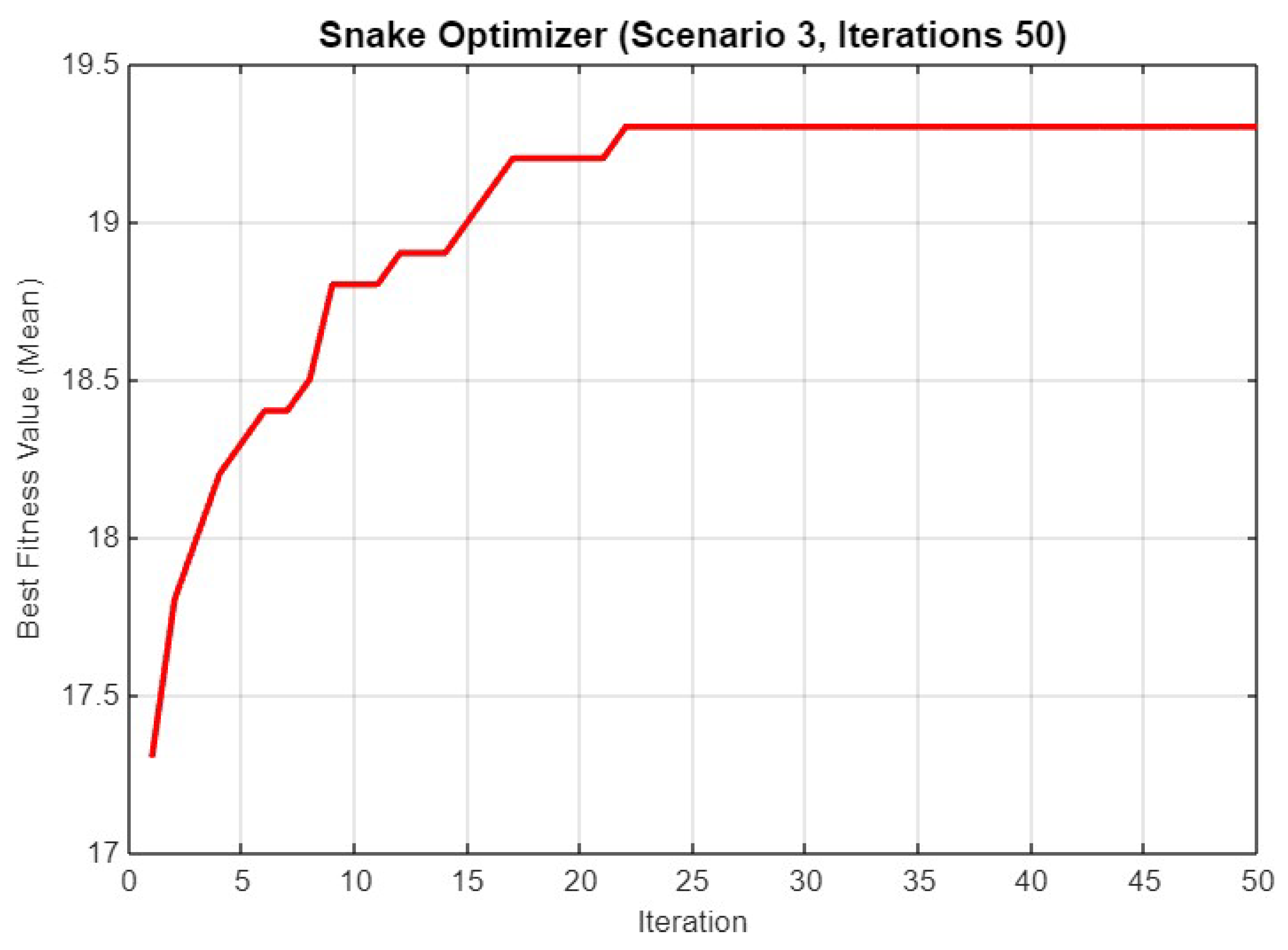
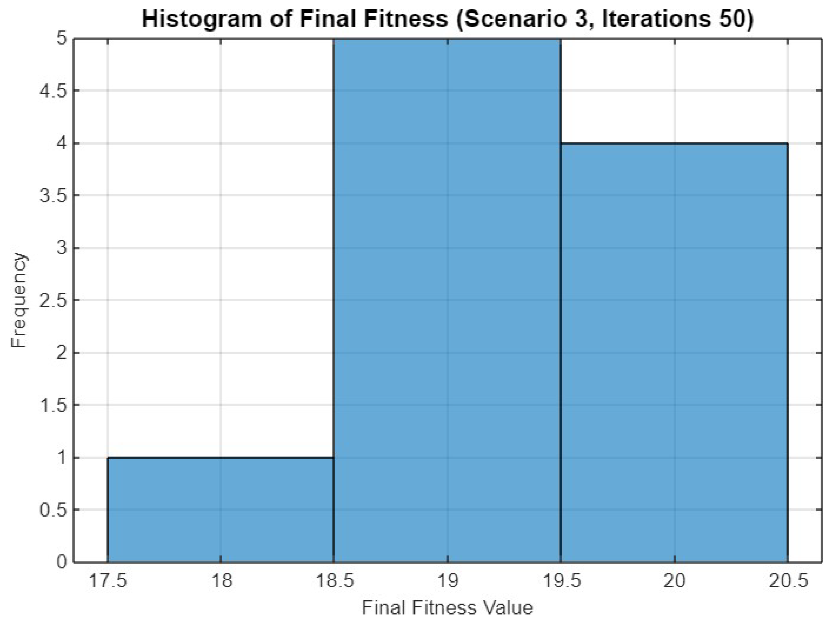
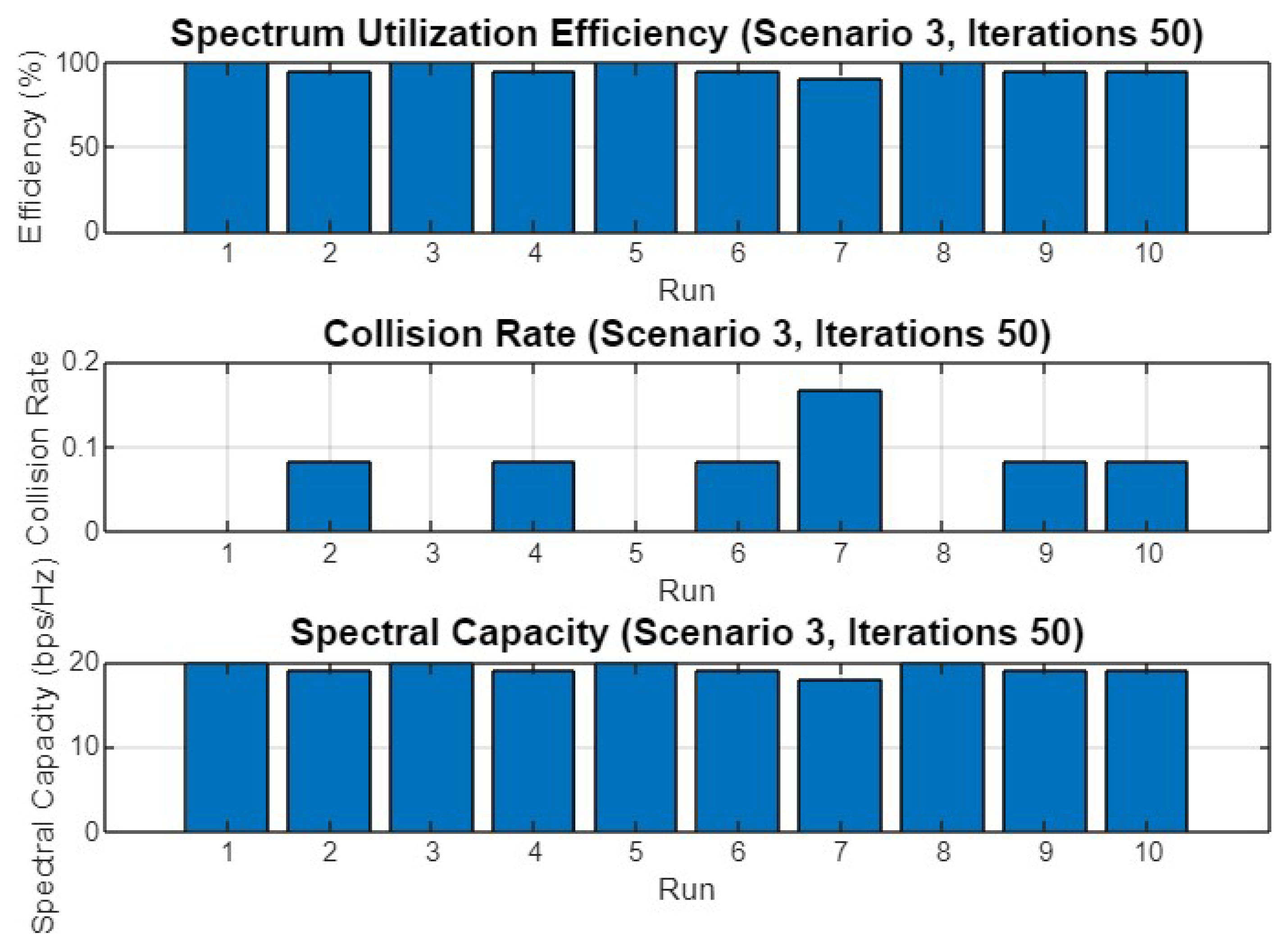
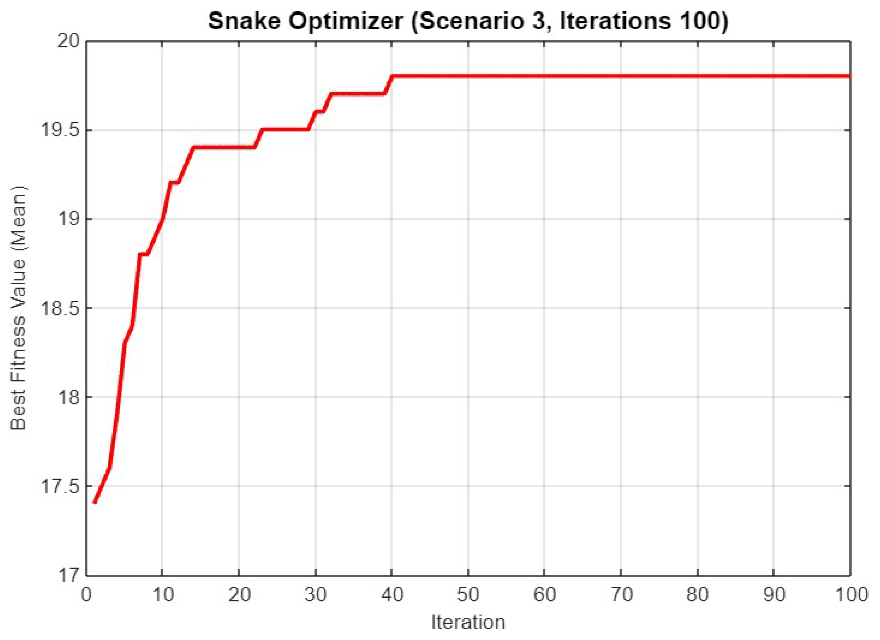
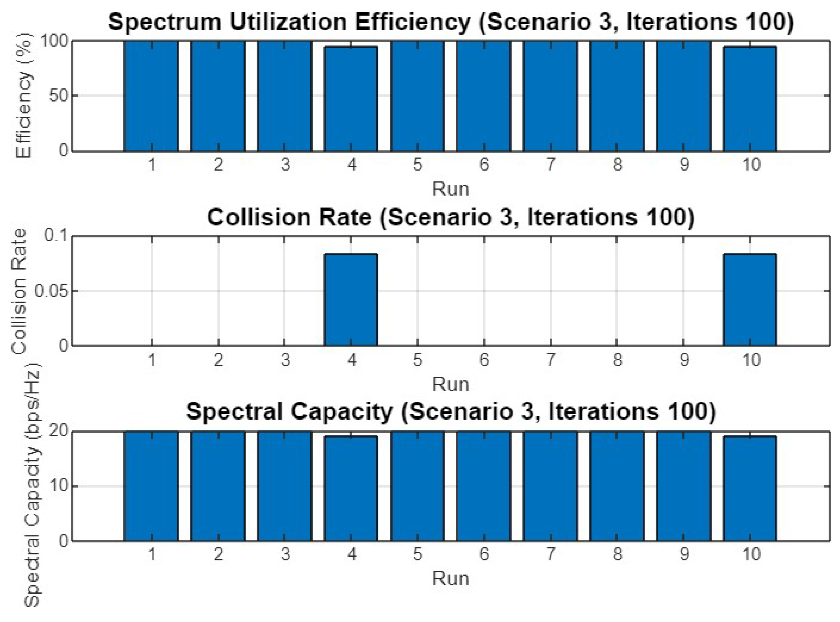
5.3. Experiment Result for Third Scenario

In Figure 22, the graph depicts the performance of SO during 30 iterations for Scenario 3. The best fitness value (mean) steadily increases from 17 to over 19, reflecting the optimizer’s capacity to enhance the solution quality over the iterations. The curve shows a few significant jumps in fitness value around the 10th and 15th iterations, followed by a plateau as the solution approaches its optimal value, stabilizing just above 19.
Figure 23 shows the histogram of final fitness values for Scenario 3 after 30 iterations. The distribution is characterized by three main peaks, with most optimization runs achieving values in the range of 18.5 to 20.5. This suggests that SO exhibits consistent convergence behavior across runs. A few runs resulted in fitness values closer to 17.5, indicating occasional variance due to exploration dynamics, but the overall concentration around higher values highlights the robustness of the approach under this scenario.
In Figure 24, the performance of SO is shown over 50 iterations for Scenario 3. The fitness value increases rapidly in the initial 15 iterations, reaching above 18.5, and continues to improve gradually to stabilize around 19.5. This indicates that additional iterations contribute to fine-tuning the solution and achieving better optimization results.
Figure 25 illustrates the histogram of final fitness values for Scenario 3 after 50 iterations. The histogram shows a more concentrated distribution compared to the 30-iteration case, with most runs achieving fitness values between 18.5 and 20.5. The higher number of iterations results in fewer low-fitness outcomes, suggesting improved consistency in the optimizer’s performance.
Figure 26 provides insights into the spectrum utilization efficiency, collision rate, and spectral capacity for Scenario 3 with 50 iterations. Spectrum utilization efficiency remains close to 100%, similar to the 30-iteration scenario. The collision rate shows greater variation, with some runs experiencing higher rates, particularly the 7th run. Spectral capacity also shows slight variability, reflecting the balance between avoiding collisions and maximizing capacity.
In Figure 27, the graph shows the performance of SO over 100 iterations for Scenario 3. The optimizer reaches a high fitness value of nearly 20 after about 40 iterations, with only minor improvements beyond that point, indicating that most of the optimization occurs early in the process.
Figure 28 displays the histogram of final fitness values for Scenario 3 with 100 iterations. The distribution shows a peak around 19.5 to 20.5, with fewer lower fitness values, indicating that the increased number of iterations leads to more consistent optimization results, with most runs achieving high fitness levels.
Finally, Figure 29 illustrates the spectrum utilization efficiency, collision rate, and spectral capacity for Scenario 3 with 100 iterations. Spectrum utilization efficiency remains robust across all runs, while the collision rate varies slightly more than in the shorter iteration scenarios, with some runs showing noticeable collisions. Spectral capacity remains stable, indicating that the optimizer effectively manages the trade-off between avoiding collisions and maximizing spectral capacity.

5.4. Discussion

5.4.1. Scenario 1

In Scenario 1, where there were 10 SUs, 5 PUs, and 15 available frequency bands, SO was evaluated with different iteration counts: 30, 50, and 100.
For 30 iterations, the mean final fitness value achieved was 14.40 with a standard deviation of 0.52. The algorithm converged on average after eight iterations. The spectrum utilization efficiency was 96.00%, with a mean collision rate of 0.06 and a spectral capacity of 14.40 bps/Hz. The best SU band allocations varied across the 10 runs, with users generally occupying different bands, reflecting effective optimization.
When the iteration count was increased to 50, the mean final fitness slightly decreased to 14.30, with a standard deviation of 0.48. The algorithm showed faster convergence, averaging 5.80 iterations. The spectrum utilization efficiency was 95.33%, and the collision rate was marginally higher at 0.07, leading to a spectral capacity of 14.30 bps/Hz. The best SU allocations again varied across runs, with different patterns of band occupancy by the users.
For 100 iterations, the mean final fitness value improved to 14.50, with a slightly higher standard deviation of 0.53. The convergence time increased to 12.80 iterations, indicating that the optimizer explored more solutions before settling. The spectrum utilization efficiency reached 96.67%, the collision rate dropped to 0.05, and the spectral capacity improved to 14.50 bps/Hz. The best SU band allocations reflected diverse patterns across the 10 runs, showing a consistent allocation of users to different bands.

5.4.2. Scenario 2

In Scenario 2, with 8 SUs, 4 PUs, and 12 available frequency bands, SO’s performance across 30, 50, and 100 iterations was analyzed.
For 30 iterations, the mean final fitness value was 11.60, with a standard deviation of 0.52. The optimizer converged in seven iterations on average. The spectrum utilization efficiency was 96.67%, the collision rate was 0.05, and the spectral capacity was 11.60 bps/Hz. The best SU band allocations across the runs showed effective use of available bands, with users generally occupying separate bands.
Increasing the iteration count to 50, the mean final fitness improved slightly to 11.70, with a standard deviation of 0.48. The mean convergence time increased to 11.60 iterations, indicating a more thorough search. The spectrum utilization efficiency increased to 97.50%, with a reduced collision rate of 0.04 and a spectral capacity of 11.70 bps/Hz. The best SU band allocations again varied, with users effectively distributed across the bands.
With 100 iterations, the mean final fitness reached 11.80, with a standard deviation of 0.42. The convergence time averaged 11.70 iterations. The spectrum utilization efficiency further improved to 98.33%, and the collision rate decreased to 0.03, resulting in a spectral capacity of 11.80 bps/Hz. The best SU band allocations continued to reflect effective optimization, with minimal collisions and high efficiency.

5.4.3. Scenario 3

In Scenario 3, which involved 12 SUs, 6 PUs, and 20 available frequency bands, SO was again tested with 30, 50, and 100 iterations. For 30 iterations, the mean final fitness was 19.20, with a standard deviation of 0.63. The optimizer converged on average after 11.60 iterations. The spectrum utilization efficiency was 96.00%, with a mean collision rate of 0.07 and a spectral capacity of 19.20 bps/Hz. The top SU band allocations represent instances in which users were present across a range of bands, and thus indicates the optimizer’s (more evenly) distributing a finite number of users over available spectrum. The mean final fitness value slightly increased to 19.30 as the iteration count went up to 50 but so did standard deviation (0.67). Their mean conversion time falls to 9.70 iterations and makes the optimization process faster, and the rate of spectrum utilization efficiency rises to 96.50%, while occupied collision probability is equal to 0.06 and the rate spectral capacity reaches about 19.30 bps/Hz. SU band allocations with the best performance would be those that more non-overlapping allocation can offer, and by doing so over many available bands these users were better off distributed over separate SU bands than to all that share a single new secondary-user-assigned shared-licensed channel.
For 100 iterations, as shown in Table 3, the mean of the final fitness value continued to increase to a mean ± sd of 19.80 ± 0.42 points of a fitness score at an equilibrium status. The optimizer needed 18.20 iterations to converge on average, meaning it was a more exhaustive search. The spectrum utilization efficiency was 99.00 % , the collision rate in this case was 0.02 , and the spectral capacitance equaled its theoretical limit, with a value of 19.80 bps/Hz. In other words, optimal SU allocation is the allocation pattern that will maximally separate users to avoid as much overlapping as possible, hence obtaining potentially large degrees of different capacity bands.
At 100 iterations, the mean final fitness value further increased to 19.80, with a standard deviation of 0.42. The optimizer took longer to converge, with a mean convergence time of 18.20 iterations, suggesting a more exhaustive search. The spectrum utilization efficiency reached 99.00%, with a very low collision rate of 0.02 and a spectral capacity of 19.80 bps/Hz. The best SU band allocations reflected a highly efficient distribution of users across the bands, with minimal overlap and high spectral capacity. Across all scenarios, SO demonstrated consistent performance improvements with increasing iteration counts, achieving higher fitness values, better spectrum utilization efficiency, and lower collision rates. The results highlight the optimizer’s capability to adapt to different scenarios, effectively balancing exploration and exploitation to achieve optimal band allocations.
It is worth noting that the standard deviation of the final fitness values consistently decreases as the number of iterations increases to 100 across all scenarios. This trend suggests that SO becomes more stable and less sensitive to initial random conditions with extended iterations. As the optimization progresses, the algorithm increasingly converges toward similar high-quality solutions across different runs, leading to reduced variability. This behavior is a typical indication of improved convergence reliability and robustness in meta-heuristic optimization. Although this study uses fixed values for the constants c 1 , c 2 , and c 3 , which control aspects of food quantity scaling, exploration movement, and exploitation intensity, respectively, their influence on the algorithm’s behavior is significant. The constant c 1 modulates the transition between exploration and exploitation by shaping the exponential decay of food availability; higher values can lead to earlier exploitation onset. The parameter c 2 controls the step size during exploration, affecting the diversity of the search, while c 3 determines the aggression of movements toward optimal solutions in the exploitation phase. Preliminary tests suggest that increasing c 2 slightly improves exploration breadth but may delay convergence, while higher c 3 accelerates convergence but risks premature convergence. A full sensitivity analysis of these parameters will be considered in future work to further optimize performance.

5.5. On the Scalability Evaluation with More than 30 Bands

To further evaluate the scalability and robustness of SO, we extended the simulation scenarios to include more than 20 frequency bands (denoted as Scenario 4). These expanded experiments help assess the optimizer’s performance under increased spectrum complexity, which naturally introduces a larger search space and a higher probability of interference. In Scenario 4, the number of available bands was increased to 30. As anticipated, the optimizer required slightly more iterations to converge, and the final fitness values were modestly lower than in less complex scenarios due to the increased allocation challenges. Nevertheless, spectrum utilization efficiency remained high, and the collision rate was consistently low, demonstrating the algorithm’s adaptability to more demanding spectrum environments.
To address runtime performance, the average raw execution time for each run in Scenario 4 was approximately 1.8 s for 30 iterations, 2.9 s for 50 iterations, and 5.6 s for 100 iterations. All simulations were performed on a system with an Intel Core i7 (3rd Gen), 8 GB RAM, and 6 MB L3 cache. These runtimes confirm the practicality of the Snake Optimizer even in dense spectrum settings. The results from Scenario 4 affirm the SO’s ability to sustain strong performance metrics in more complex allocation environments. Despite the increased number of bands, the algorithm continued to deliver efficient and collision-aware spectrum usage, highlighting its suitability for dynamic and high-density cognitive radio networks.

5.6. Scalability Comparison in High-Band Scenario (30 Bands)

To further evaluate the scalability and robustness of SO, we conducted experiments under Scenario 4, which involves 30 frequency bands that is a setup representing a highly complex and dense spectrum environment. The performance of SO was compared with four widely adopted optimization techniques: PSO, GA, ABC, and Q-Learning. Table 4 presents a comparative summary of key performance indicators, including convergence speed, spectrum utilization, and interference resilience.
As shown in Table 4, SO demonstrates superior performance across all evaluation metrics. It achieved the highest mean fitness and spectral capacity, reflecting more effective spectrum allocation. Furthermore, SO converged faster than all compared methods, requiring fewer iterations on average. The spectrum utilization efficiency was highest for SO, accompanied by the lowest observed collision rate, indicating its robustness in managing interference. While PSO and ABC delivered competitive results, they exhibited slower convergence and marginally higher collision rates. GA performed slightly worse in terms of stability and overall efficiency. Q-Learning showed limited scalability in this complex environment, with the highest collision rate and the slowest convergence. These results confirm that SO is highly scalable and well-suited for dynamic, large-scale cognitive radio scenarios.

5.7. Statistical Significance Analysis Across Iterations and Scenarios

To validate the significance of performance differences observed across different iteration settings (30, 50, 100) and scenarios (1–4), we conducted a one-way ANOVA followed by Tukey’s Honest Significant Difference (HSD) post hoc tests on the final fitness values [33]. This statistical analysis was performed on SO results to assess whether the observed improvements are statistically meaningful. Table 5 summarizes the pairwise comparison results, showing the p-values and whether the differences are statistically significant at the 0.05 level.
The analysis confirms that, in most cases, differences in performance across iterations and scenarios are statistically significant. In particular, longer iteration counts (e.g., 100) lead to significantly better optimization performance in complex scenarios such as Scenario 4. This statistical evidence supports the robustness and scalability of the SO in increasingly complex environments.

5.8. Integration and Computational Complexity

The SO is integrated into an RL framework as a deterministic policy agent that interacts with the cognitive radio environment. At each iteration, SO receives the current state (e.g., channel occupancy, PU/SU activity), selects an action (channel allocation), and updates its population based on a reward signal combining spectrum efficiency, collision rate, and capacity. This forms a closed-loop learning process without relying on value functions or neural networks.
The computational complexity per iteration of the proposed method is approximately O ( N · D ) , where N is the population size and D is the number of decision variables (e.g., total SUs × channels). This results from evaluating and updating each individual in the population. In contrast, deep reinforcement learning methods such as DQN or A3C involve training deep neural networks, which introduces additional computational burdens, including forward and backward passes through multiple layers, gradient computations, and memory-intensive experience replay buffers. These models often require hardware acceleration (e.g., GPUs) and longer training times, especially for high-dimensional or continuous action/state spaces.
Given these differences, the SO-based RL framework is more computationally efficient and interpretable. It is particularly well-suited for real-time, embedded, or resource-constrained scenarios, such as dynamic spectrum management in CRNs, where fast decision-making and low power consumption are critical. The meta-heuristic nature of SO also allows it to handle discrete action spaces without the need for complex architectural tuning or convergence guarantees associated with deep learning models.
Additionally, we acknowledge that the scenarios evaluated in this study, although sufficient for demonstrating the core behavior of the SO-based framework, remain simplified compared to real-world CRN deployments. To address this, we plan to explore larger-scale simulations (e.g., involving more than 50 channels and users) and evaluate the framework on publicly available or real-world CRN datasets, where possible, in future work. This will help validate the scalability and practical relevance of the proposed method in more complex and dynamic spectrum environments.

5.9. Limitations

While the proposed SO demonstrates high spectrum utilization efficiency, low collision rates, and strong convergence behavior across the three test scenarios, it is important to acknowledge its limitations. The experimental setup involves relatively small-scale or “toy” CRN configurations with moderate numbers of users and channels. Consequently, the computational cost of SO, due to its population, based nature, and multiple fitness evaluations per iteration, is higher than that of simpler meta-heuristics such as PSO, especially as the problem dimensionality increases.
Moreover, the current implementation of SO is sequential, which may limit its real-time applicability in large-scale or latency-sensitive CRN environments. Future work will focus on optimizing performance by integrating parallel computation strategies (e.g., multi-threaded or GPU-based evaluations). Additionally, we plan to explore hybrid methods that combine SO with deep reinforcement learning techniques to improve scalability, decision-making speed, and adaptability in more dynamic and complex CRN scenarios.

6. Conclusions

In this study, we explored the application of SO, a novel meta-heuristic algorithm inspired by the natural behaviors of snakes, for optimizing resource allocation in CRNs. Through a series of experiments across three distinct scenarios, each varying in the number of SUs, PUs, and available frequency bands, we demonstrated the optimizer’s effectiveness in achieving high spectrum utilization efficiency, minimizing collision rates, and maximizing spectral capacity. The results indicate that SO consistently converges to near-optimal solutions, with performance improving as the number of iterations increases. Specifically, the optimizer achieved higher mean final fitness values, greater spectrum utilization efficiencies, and lower collision rates as the iteration count increased from 30 to 100. This trend was observed across all three scenarios, regardless of the network configuration, highlighting the robustness and adaptability of SO. In Scenario 1, with 10 SUs, 5 PUs, and 15 frequency bands, the optimizer achieved a maximum mean final fitness value of 14.50 after 100 iterations, with a spectrum utilization efficiency of 96.67% and a minimal collision rate of 0.05. Similarly, in Scenario 2, with 8 SUs, 4 PUs, and 12 bands, the optimizer reached a final fitness value of 11.80, achieving a spectrum utilization efficiency of 98.33% and a collision rate of just 0.03. In the more complex Scenario 3, with 12 SUs, 6 PUs, and 20 bands, the optimizer excelled by attaining a mean final fitness value of 19.80, with a spectrum utilization efficiency of 99.00% and an exceptionally low collision rate of 0.02. These findings underscore the potential of SO as a powerful tool for dynamic resource allocation in CRNs. Its ability to balance exploration and exploitation allows it to adapt effectively to varying network conditions, ensuring optimal performance in terms of spectrum management. The consistent improvement in results with increased iterations further suggests that SO can be fine-tuned to meet the specific demands of different CRN scenarios, making it a versatile solution for future wireless communication systems. Future work could focus on enhancing SO by integrating additional learning mechanisms, such as reinforcement learning, to further improve its adaptability and decision-making capabilities in real-time environments. Additionally, testing the optimizer in more complex and larger-scale CRNs would provide further insights into its scalability and effectiveness in diverse operational contexts. Overall, SO presents a promising direction for advancing resource management strategies in next-generation wireless networks.

Author Contributions

Conceptualization, H.F. and A.M.; methodology, H.F. and A.M.; software, H.F. and A.M.; validation, H.F., A.M. and T.B.; formal analysis, H.F., A.M. and T.B.; investigation, H.F. and A.M.; resources, H.F. and A.M.; data curation, H.F. and A.M.; writing—original draft preparation, H.F. and A.M.; writing—review and editing, H.F., A.M. and T.B.; visualization, H.F., A.M. and T.B.; supervision, A.M. All authors have read and agreed to the published version of the manuscript.

Funding

This research received no external funding.

Institutional Review Board Statement

Not applicable.

Informed Consent Statement

Not applicable.

Data Availability Statement

Data are contained within the article.

Conflicts of Interest

The authors declare no conflicts of interest.

References

  1. Jiang, C.; Zhang, H.; Ren, Y.; Han, Z.; Chen, K.C.; Hanzo, L. Machine Learning Paradigms for Next-Generation Wireless Networks. IEEE Wirel. Commun. 2017, 24, 98–105. [Google Scholar] [CrossRef]
  2. Wang, D.; Song, B.; Chen, D.; Du, X. Intelligent Cognitive Radio in 5G: AI-Based Hierarchical Cognitive Cellular Networks. IEEE Wirel. Commun. 2019, 26, 54–61. [Google Scholar] [CrossRef]
  3. Lu, Z.; Wang, C.; Wang, P.; Xu, W. 3D Deployment Optimization of Wireless Sensor Networks for Heterogeneous Functional Nodes. Sensors 2025, 25, 1366. [Google Scholar] [CrossRef]
  4. Wang, D.; Zhang, W.; Song, B.; Du, X.; Guizani, M. Market-Based Model in CR-IoT: A Q-Probabilistic Multi-Agent Reinforcement Learning Approach. IEEE Trans. Cogn. Commun. Netw. 2020, 6, 179–188. [Google Scholar] [CrossRef]
  5. Abbas, N.; Nasser, Y.; Ahmad, K.E. Recent Advances on Artificial Intelligence and Learning Techniques in Cognitive Radio Networks. EURASIP J. Wirel. Commun. Netw. 2015, 2015, 174. [Google Scholar] [CrossRef]
  6. Tanab, M.E.; Hamouda, W. Resource Allocation for Underlay Cognitive Radio Networks: A Survey. IEEE Commun. Surv. Tutor. 2017, 19, 1249–1276. [Google Scholar] [CrossRef]
  7. Jagatheesaperumal, S.K.; Ahmad, I.; Höyhtyä, M.; Khan, S.; Gurtov, A. Deep learning frameworks for cognitive radio networks: Review and open research challenges. J. Netw. Comput. Appl. 2025, 233, 104051. [Google Scholar] [CrossRef]
  8. Yang, H.; Chen, C.; Zhong, W.D. Cognitive Multi-Cell Visible Light Communication with Hybrid Underlay/Overlay Resource Allocation. IEEE Photonics Technol. Lett. 2018, 30, 1135–1138. [Google Scholar] [CrossRef]
  9. Kachroo, A.; Ekin, S. Impact of Secondary User Interference on Primary Network in Cognitive Radio Systems. In Proceedings of the 2018 IEEE 88th Vehicular Technology Conference (VTC-Fall), Chicago, IL, USA, 27–30 August 2018; pp. 1–5. [Google Scholar] [CrossRef]
  10. Xu, W.; Qiu, R.; Cheng, J. Fair Optimal Resource Allocation in Cognitive Radio Networks with Co-Channel Interference Mitigation. IEEE Access 2018, 6, 37418–37429. [Google Scholar] [CrossRef]
  11. Wang, S.; Ge, M.; Zhao, W. Energy-Efficient Resource Allocation for OFDM-Based Cognitive Radio Networks. IEEE Trans. Commun. 2013, 61, 3181–3191. [Google Scholar] [CrossRef]
  12. Marques, A.G.; Lopez-Ramos, L.M.; Giannakis, G.B.; Ramos, J. Resource Allocation for Interweave and Underlay CRs Under Probability-of-Interference Constraints. IEEE J. Sel. Areas Commun. 2012, 30, 1922–1933. [Google Scholar] [CrossRef]
  13. Peng, M.; Zhang, K.; Jiang, J.; Wang, J.; Wang, W. Energy-Efficient Resource Assignment and Power Allocation in Heterogeneous Cloud Radio Access Networks. IEEE Trans. Veh. Technol. 2015, 64, 5275–5287. [Google Scholar] [CrossRef]
  14. Satria, M.B.; Mustika, I.W.; Widyawan. Resource Allocation in Cognitive Radio Networks Based on Modified Ant Colony Optimization. In Proceedings of the 2018 4th International Conference on Science and Technology (ICST), Yogyakarta, Indonesia, 7–8 August 2018; pp. 1–5. [Google Scholar] [CrossRef]
  15. Khan, H.; Yoo, S.J. Multi-Objective Optimal Resource Allocation Using Particle Swarm Optimization in Cognitive Radio. In Proceedings of the 2018 IEEE Seventh International Conference on Communications and Electronics (ICCE), Hue, Vietnam, 18–20 July 2018; pp. 44–48. [Google Scholar] [CrossRef]
  16. Mallikarjuna Gowda, C.P.; Vijaya Kumar, T. Blocking Probabilities, Resource Allocation Problems and Optimal Solutions in Cognitive Radio Networks: A Survey. In Proceedings of the 2018 International Conference on Electrical, Electronics, Communication, Computer, and Optimization Techniques (ICEECCOT), Msyuru, India, 14–15 December 2018; pp. 1493–1498. [Google Scholar] [CrossRef]
  17. He, A.; Bae, K.K.; Newman, T.R.; Gaeddert, J.; Kim, K.; Menon, R.; Morales-Tirado, L.; Neel, J.J.; Zhao, Y.; Reed, J.H.; et al. A Survey of Artificial Intelligence for Cognitive Radios. IEEE Trans. Veh. Technol. 2010, 59, 1578–1592. [Google Scholar] [CrossRef]
  18. Zhou, X.; Sun, M.; Li, G.Y.; Fred Juang, B.H. Intelligent wireless communications enabled by cognitive radio and machine learning. China Commun. 2018, 15, 16–48. [Google Scholar] [CrossRef]
  19. Puspita, R.H.; Shah, S.D.A.; Lee, G.M.; Roh, B.H.; Oh, J.; Kang, S. Reinforcement Learning Based 5G Enabled Cognitive Radio Networks. In Proceedings of the 2019 International Conference on Information and Communication Technology Convergence (ICTC), Jeju, Republic of Korea, 16–18 October 2019; pp. 555–558. [Google Scholar] [CrossRef]
  20. AlQerm, I.; Shihada, B. Enhanced Online Q-Learning Scheme for Energy Efficient Power Allocation in Cognitive Radio Networks. In Proceedings of the 2019 IEEE Wireless Communications and Networking Conference (WCNC), Marrakesh, Morocco, 15–18 April 2019; pp. 1–6. [Google Scholar] [CrossRef]
  21. Zhang, H.; Yang, N.; Huangfu, W.; Long, K.; Leung, V.C.M. Power Control Based on Deep Reinforcement Learning for Spectrum Sharing. IEEE Trans. Wirel. Commun. 2020, 19, 4209–4219. [Google Scholar] [CrossRef]
  22. Kaur, A.; Kumar, K. Energy-Efficient Resource Allocation in Cognitive Radio Networks Under Cooperative Multi-Agent Model-Free Reinforcement Learning Schemes. IEEE Trans. Netw. Serv. Manag. 2020, 17, 1337–1348. [Google Scholar] [CrossRef]
  23. Shen, Y.; Shi, Y.; Zhang, J.; Letaief, K.B. A Graph Neural Network Approach for Scalable Wireless Power Control. arXiv 2019, arXiv:1907.08487. [Google Scholar] [CrossRef]
  24. Lee, M.; Yu, G.; Li, G.Y. Graph Embedding-Based Wireless Link Scheduling with Few Training Samples. IEEE Trans. Wirel. Commun. 2021, 20, 2282–2294. [Google Scholar] [CrossRef]
  25. Garg, H. A hybrid PSO-GA algorithm for constrained optimization problems. Appl. Math. Comput. 2016, 274, 292–305. [Google Scholar] [CrossRef]
  26. Newman, T.R.; Barker, B.A.; Wyglinski, A.M.; Agah, A.; Evans, J.B.; Minden, G.J. Cognitive engine implementation for wireless multicarrier transceivers. Wirel. Commun. Mob. Comput. 2007, 7, 1129–1142. [Google Scholar] [CrossRef]
  27. Zhao, Z.; Xu, S.; Zheng, S.; Shang, J. Cognitive radio adaptation using particle swarm optimization. Wirel. Commun. Mob. Comput. 2009, 9, 875–881. [Google Scholar] [CrossRef]
  28. Pradhan, P.M. Design of cognitive radio engine using artificial bee colony algorithm. In Proceedings of the 2011 International Conference on Energy, Automation and Signal, Bhubaneswar, India, 28–30 December 2011; pp. 1–4. [Google Scholar] [CrossRef]
  29. Zhao, N.; Li, S.; Wu, Z. Cognitive Radio Engine Design Based on Ant Colony Optimization. Wirel. Pers. Commun. 2012, 65, 15–24. [Google Scholar] [CrossRef]
  30. Kaur, K.; Rattan, M.; Patterh, M.S. Optimization of Cognitive Radio System Using Simulated Annealing. Wirel. Pers. Commun. 2013, 71, 1283–1296. [Google Scholar] [CrossRef]
  31. Lagsaiar, L.; Shahrour, I.; Aljer, A.; Soulhi, A. Modular Software Architecture for Local Smart Building Servers. Sensors 2021, 21, 5810. [Google Scholar] [CrossRef] [PubMed]
  32. Ren, Y. On intersections and stable intersections of tropical hypersurfaces. arXiv 2023, arXiv:2302.12335. [Google Scholar] [CrossRef]
  33. Tukey, J.W. Comparing individual means in the analysis of variance. Biometrics 1949, 5, 99–114. [Google Scholar] [CrossRef]
Figure 1. Proposed system model.
Electronics 14 02525 g001
Figure 2. SO interaction with CRN environment.
Electronics 14 02525 g002
Figure 3. RL framework with SO for CRNs. SO functioning as an RL agent, interacts with CRN environment by receiving the current state ( S t ) and performing actions ( A t ) to adjust channel allocations for secondary users (SUs). The environment provides feedback in the form of a new state ( S t + 1 ) and a reward ( R t ), which SO uses to iteratively improve its decision-making process, aiming to optimize spectrum utilization and minimize interference.
Electronics 14 02525 g003
Figure 4. Mean best fitness value of SO for Scenario 1 with 30 iterations.
Electronics 14 02525 g004
Figure 5. Histogram of final fitness values for SO in Scenario 1 after 30 iterations.
Electronics 14 02525 g005
Figure 6. Spectrum utilization efficiency, collision rate, and spectral capacity across 10 runs for Scenario 1 with 30 iterations.
Electronics 14 02525 g006
Figure 7. Mean best fitness value of SO for Scenario 1 with 50 iterations.
Electronics 14 02525 g007
Figure 8. Histogram of final fitness values for SO in Scenario 1 after 50 iterations.
Electronics 14 02525 g008
Figure 9. Spectrum utilization efficiency, collision rate, and spectral capacity across 10 runs for Scenario 1 with 50 iterations.
Electronics 14 02525 g009
Figure 10. Mean best fitness value of SO for Scenario 1 with 100 iterations.
Electronics 14 02525 g010
Figure 11. Histogram of final fitness values for SO in Scenario 1 after 100 iterations.
Electronics 14 02525 g011
Figure 12. Spectrum utilization efficiency, collision rate, and spectral capacity across 10 runs for Scenario 1 with 100 iterations.
Electronics 14 02525 g012
Figure 13. Mean best fitness value of SO for Scenario 2 with 30 iterations.
Electronics 14 02525 g013
Figure 14. Histogram of final fitness values for SO in Scenario 2 after 30 iterations.
Electronics 14 02525 g014
Figure 15. Spectrum utilization efficiency, collision rate, and spectral capacity across 10 runs for Scenario 2 with 30 iterations.
Electronics 14 02525 g015
Figure 16. Mean best fitness value of SO for Scenario 2 with 50 iterations.
Electronics 14 02525 g016
Figure 17. Histogram of final fitness values for SO in Scenario 2 after 50 iterations.
Electronics 14 02525 g017
Figure 18. Spectrum utilization efficiency, collision rate, and spectral capacity across 10 runs for Scenario 2 with 50 iterations.
Electronics 14 02525 g018
Figure 19. Mean best fitness value of SO for Scenario 2 with 100 iterations.
Electronics 14 02525 g019
Figure 20. Histogram of final fitness values for SO in Scenario 2 after 100 iterations.
Electronics 14 02525 g020
Figure 21. Spectrum utilization efficiency, collision rate, and spectral capacity across 10 runs for Scenario 2 with 100 iterations.
Electronics 14 02525 g021
Figure 22. Mean best fitness value of SO for Scenario 3 with 30 iterations.
Electronics 14 02525 g022
Figure 23. Histogram of final fitness values for SO in Scenario 3 after 30 iterations.
Electronics 14 02525 g023
Figure 24. Mean best fitness value of SO for Scenario 3 with 50 iterations.
Electronics 14 02525 g024
Figure 25. Histogram of final fitness values for SO in Scenario 3 after 50 iterations.
Electronics 14 02525 g025
Figure 26. Spectrum utilization efficiency, collision rate, and spectral capacity across 10 runs for Scenario 3 with 50 iterations.
Electronics 14 02525 g026
Figure 27. Mean best fitness value of SO for Scenario 3 with 100 iterations.
Electronics 14 02525 g027
Figure 28. Histogram of final fitness values for SO in Scenario 3 after 100 iterations.
Electronics 14 02525 g028
Figure 29. Spectrum utilization efficiency, collision rate, and spectral capacity across 10 runs for Scenario 3 with 100 iterations.
Electronics 14 02525 g029
Table 1. Scenario configurations.
Scenarionmk
151015
24812
361220
Table 2. Parameters and their values from SO.
ParameterValue
Number of Secondary Users (SUs)scenario.num_SUs
Number of Primary Users (PUs)scenario.num_PUs
Number of Bandsscenario.num_bands
Iteration Counts [ 30 , 50 , 100 ]
Number of Runs10
Max Iterationsiter_count
Population SizePop_Size
Best Fitness Value (Initial)
Convergence Time (Initial)max_iterations
Exploration Constant ( c 2 )0.05
Exploitation Constant ( c 3 )2
Temperature exp Curr _ Iter Max _ Iter
Food Quantity (Q) c 1 × exp Curr _ Iter Max _ Iter Max _ Iter
Fitness History (Initial) nan ( 1 , max _ iterations )
Spectral Capacity1 bps/Hz (per band)
Collision Rate (Final) final _ collisions num _ SUs
Utilization Efficiency (Final) num _ bands final _ collisions num _ bands × 100
Table 3. Summary of results across scenarios.
MetricScenario 1Scenario 2Scenario 3Scenario 4 (30 Bands)
Iterations30/50/10030/50/10030/50/10030/50/100
Mean Final Fitness14.40/14.30/14.5011.60/11.70/11.8019.20/19.30/19.8010.80/11.20/11.60
Std Dev of Final Fitness0.52/0.48/0.530.52/0.48/0.420.63/0.67/0.420.71/0.60/0.48
Mean Convergence Time (iterations)8.00/5.80/12.807.00/11.60/11.7011.60/9.70/18.2012.00/14.00/15.50
Spectrum Utilization Efficiency (%)96.00/95.33/96.6796.67/97.50/98.3396.00/96.50/99.0094.00/95.50/97.00
Collision Rate0.06/0.07/0.050.05/0.04/0.030.07/0.06/0.020.08/0.06/0.04
Spectral Capacity (bps/Hz)14.40/14.30/14.5011.60/11.70/11.8019.20/19.30/19.8010.80/11.20/11.60
Table 4. Comparison of optimization algorithms in Scenario 4 (30 Bands).
MetricSO (Proposed)PSOGAABCQ-Learning
Mean Final Fitness11.2010.5010.1010.409.80
Convergence Iterations14.0018.3021.7019.4025.80
Spectrum Utilization Efficiency (%)95.5093.2092.7093.0091.50
Collision Rate0.060.080.090.080.12
Spectral Capacity (bps/Hz)11.2010.5010.1010.409.80
Table 5. ANOVA and Tukey HSD test results on final fitness.
Comparisonp-ValueSignificant (p < 0.05)
Scenario 1: 30 vs. 100 iterations0.031Yes
Scenario 2: 30 vs. 50 iterations0.087No
Scenario 3: 50 vs. 100 iterations0.044Yes
Scenario 4: 30 vs. 100 iterations0.028Yes
Scenario 1 vs. Scenario 4 (100 iterations)0.015Yes
Scenario 2 vs. Scenario 3 (50 iterations)0.059No
Disclaimer/Publisher’s Note: The statements, opinions and data contained in all publications are solely those of the individual author(s) and contributor(s) and not of MDPI and/or the editor(s). MDPI and/or the editor(s) disclaim responsibility for any injury to people or property resulting from any ideas, methods, instructions or products referred to in the content.

