Cost-Optimised Machine Learning Model Comparison for Predictive Maintenance

Abstract

Predictive maintenance is essential for reducing industrial downtime and costs, yet real-world datasets frequently encounter class imbalance and require cost-sensitive evaluation due to costly misclassification errors. This study utilises the SCANIA Component X dataset to advance predictive maintenance through machine learning, employing seven supervised algorithms, Support Vector Machine, Random Forest, Decision Tree, K-Nearest Neighbours, Multi-Layer Perceptron, XGBoost, and LightGBM, trained on time-series features extracted via a sliding window approach. A bespoke cost-sensitive metric, aligned with SCANIA’s misclassification cost matrix, assesses model performance. Three imbalance mitigation strategies, downsampling, downsampling with SMOTETomek, and manual class weighting, were explored, with downsampling proving most effective. Random Forest and Support Vector Machine models achieved high accuracy and low misclassification costs, whilst a voting ensemble further enhanced cost efficiency. This research emphasises the critical role of cost-aware evaluation and imbalance handling, proposing an ensemble-based framework to improve predictive maintenance in industrial applications

1. Introduction

As a fundamental aspect of the industrial sector, maintenance plays a crucial role in production costs, making well-structured strategies essential to minimise unplanned downtime, reduce expenses, and extend the lifespan of industrial machinery [1]. As illustrated in Figure 1, the evolution of maintenance strategies has transitioned from reactive approaches, where failures were addressed only after their occurrence, to preventive methods based on scheduled interventions [1]. With the advent of sensor technologies and monitoring equipment, this progression led to the adoption of condition-based maintenance (CBM), where maintenance decisions are guided by actual equipment condition. This is followed by predictive maintenance (PdM), which is widely used today, using the integration of IoT, machine learning, big data, and other advanced technologies to predict equipment failures before they occur [2,3].

Despite the advances in machine learning for PdM, developing predictive models that are both accurate and cost-efficient remains a challenge particularly when applied to real-world industrial datasets. These datasets are often imbalanced, with failure cases representing only a small fraction of the observations. In high-stakes environments, misclassification carries unequal consequences; some failures are far more costly than others. Conventional evaluation metrics such as accuracy and F1-score may therefore be insufficient to capture the real-world implications of model predictions. As such, there is a growing need to use cost-aware evaluation frameworks and to rigorously address class imbalance when designing predictive models for industrial applications.

This research investigates the use of supervised machine learning models to predict failures of a specific vehicle component, referred to as Component X, using the SCANIA Component X dataset. Seven widely used classification algorithms are implemented—Support Vector Machine (SVM), Random Forest (RF), Decision Tree (DT), K-Nearest Neighbour (KNN), Multi-Layer Perceptron (MLP), XGBoost, and LightGBM. These models are trained on features extracted via a sliding window and time-series processing pipeline, and are evaluated using a cost-sensitive metric derived from the SCANIA misclassification cost matrix.

The study is focused on investigating the following research questions(RQs);

• RQ1: To what extent can machine learning models accurately predict failures of Component X in a cost-sensitive setting?
• RQ2: Which class imbalance handling strategy yields better overall performance?
• RQ3: Which predictive model provides the optimal trade-off between classification performance and misclassification cost?

2. Background

2.1. Predictive Maintenance (PdM) Approaches

Predictive maintenance approaches have also evolved significantly and can be broadly categorised into three types: Knowledge-based approaches rely on expert knowledge and reasoning processes to diagnose and predict faults, including three main sub-methodologies: Ontology-based approaches formalise system context by defining hierarchical relationships between components and failure modes, enabling knowledge sharing, logical inference, and reuse across applications such as marine diagnostics and industrial asset monitoring [4,5,6]. Rule-based systems, commonly implemented as Expert Systems, operate by evaluating real-time monitoring data against predetermined expert-defined rules. On the other hand, model-based techniques use mathematical representations of physical processes, utilizing residuals to assess discrepancies between measured and expected behaviour. Collectively, these approaches prioritise interpretability and compliance with industrial standards, but are constrained by scalability, dependency on accurate models or exhaustive expertise, and limited adaptability to dynamic operational conditions [3,7]. Data-driven approaches have become more prevalent due to their scalability and adaptability. Research spans traditional statistical methods to deep learning for diagnostic and prognostic applications. Machine learning techniques like Random Forest, Decision Trees, Support Vector Machines, and K-Nearest Neighbours show promise in PdM systems for fault detection, root cause diagnosis, and equipment degradation forecasting [7,8,9]. Some common architectures include Auto-Encoders (AEs) for dimensionality reduction and feature extraction [10]; Convolutional Neural Networks (CNNs) for hierarchical feature learning from raw sensor data [11]; and Recurrent Neural Networks (RNNs), particularly LSTM variants, for capturing temporal dependencies in sequential data [12].

Hybrid approaches combine the strengths of multiple methodologies to achieve more robust and effective maintenance solutions. Physics-informed machine learning integrates domain knowledge and physical principles with data-driven models, enabling more reliable predictions while requiring less training data and providing better generalization capabilities [13]. Multi-modal fusion strategies integrate diverse data sources, like vibration analysis and thermal imaging, or combine physics-based models with deep learning [14]. These hybrid approaches address data scarcity and scalability limitations but require more expertise and computational resources for effective implementation [15].

2.2. Data-Driven Predictive Maintenance Framework

This research examines machine learning in predictive maintenance (PdM), outlining a four-stage data-driven framework. It begins with data acquisition and storage, systematically collecting diverse data types like sensor measurements (vibration, temperature, pressure, acoustic signals), operational data (speed, load, runtime), and maintenance records. A robust storage infrastructure ensures data integrity, quality, and real-time streaming capabilities [11,16].

2.3. Current Challenges in Predictive Maintenance Implementation

Predictive maintenance (PdM) faces challenges like cost–benefit constraints, requiring significant investment in sensors and expertise [17,18]. Data quality issues, such as incomplete or noisy datasets, hinder reliability [19]. Reliance on human operators limits proactive maintenance, and deployment is complicated by IT–researcher disconnect and data verification issues [20]. Proposed solutions include ROI calculations for cost justification, integrated IT planning, robust feedback loops, and sophisticated update cycles to prevent concept drift [2,18].

Despite the widespread adoption of PdM, its implementation is hindered by several challenges. As highlighted by [2], four key obstacles exist: The first is the cost–benefit constraint, particularly when PdM is introduced as a new investment. Expenses may arise from sensor installation, data acquisition, model development, and maintenance activities, with costs varying based on equipment complexity, sensor requirements, and the availability of in-house expertise [17,18]. The second challenge stems from PdM’s strong reliance on data availability and quality. Companies often begin with incomplete datasets when implementing production process management. Issues such as inaccurate sensor readings, data degradation and noise—particularly when sensors operate offline—must be addressed to ensure reliable PdM [19]. The third challenge concerns the continued reliance on human operators for control and maintenance. Since most industrial machines lack sufficient autonomy and self-maintenance capabilities, they typically operate reactively rather than proactively. The fourth challenge pertains to deployment in industrial settings. Integration difficulties arise because IT departments, responsible for implementation, are often separate from the researchers and developers who design the models. This separation creates obstacles, such as difficulties during the implementation stage, as organisations struggle to establish effective feedback loops for continuous model retraining. These loops can introduce risks when the integrity and relevance of incoming data are not properly verified, potentially leading to outliers contaminating the training set. Similarly, the updating phase presents challenges, as preventing concept drift during updates is significantly more complex than traditional software updates, further complicating industrial deployment [20]. Correspondingly, several approaches have been proposed to address these challenges: For cost–benefit constraints, companies can utilise projected ROI calculations to justify investments [18]. Deployment challenges can be overcome through integrated IT infrastructure planning that aligns development and implementation teams, robust data verification mechanisms in feedback loops to prevent outlier contamination, and sophisticated update cycles that simultaneously manage code, model, and data modifications to prevent concept drift [2].

2.4. Machine Learning in Predictive Maintenance

As examined in the preceding section, machine learning has been extensively applied in PdM owing to its capacity to reveal concealed patterns and early indicators of equipment degradation. This section will further explore the fundamental concepts and practical applications of machine learning in PdM. Machine learning approaches can be classified into five major categories: supervised, unsupervised, semi-supervised, self-supervised, and reinforcement learning. These approaches differ in their learning mechanisms. Unsupervised learning autonomously identifies patterns within unlabelled data, whereas semi-supervised learning uses a combination of labelled and unlabelled data to enhance model performance. Supervised learning, which is the most widely applied approach in practice, relies on labelled training data to establish input–output mappings through iterative adjustments until achieving an optimal level of accuracy for both training and unseen data predictions. Self-supervised learning, by contrast, enables models to learn from the data itself without requiring explicitly labelled examples. Reinforcement learning, on the other hand, adopts a trial-and-error approach, guided by predefined rules, to determine optimal actions [21].

2.4.1. Common Algorithms and Their Applications in Predictive Maintenance

A range of machine learning algorithms have been applied in predictive maintenance (PdM) tasks across diverse industrial domains. This section reviews how these algorithms have been applied specifically in PdM use cases, alongside their practical strengths and limitations, as identified in five widely cited survey studies [3,8,22,23,24].

Various machine learning techniques are applied in predictive maintenance (PdM). K-means clustering categorizes vibration data for fault detection but struggles with optimal cluster selection and temporal dependencies [25,26]. K-Nearest Neighbours (KNN) excels in anomaly detection and RUL estimation but is sensitive to noise and high-dimensional data [21,27]. Decision Trees (DTs) aid fault diagnosis with interpretability but risk overfitting without pruning or ensemble methods [22,28]. Random Forests (RFs) handle high-dimensional data and imbalanced datasets effectively, though computational complexity is a drawback [22,29]. Support Vector Machines (SVMs) perform well in fault classification but require extensive preprocessing for time-series data [23,30]. Gradient Boosting Machines (GBMs) model complex relationships but demand careful hyperparameter tuning [31,32]. Long Short-Term Memory (LSTM) networks manage temporal dependencies for RUL estimation but face computational and explainability challenges [33,34]. Convolutional Neural Networks (CNNs) process 1D/2D data for fault diagnosis, reducing preprocessing needs and overfitting through weight sharing [35]. Each method offers unique strengths and limitations, necessitating tailored applications in PdM.

2.4.2. Related Work on Predictive Maintenance Using SCANIA Component X Dataset

Strict data privacy policies by manufacturers limit access to real-world PdM data, pushing researchers toward synthetic datasets like NASA’s C-MAPSS, which often lack real-world complexity [36]. The SCANIA Component X dataset, with its multivariate time series from truck operations, offers a breakthrough for PdM research. Meanwhile, [37] explored Graph Neural Networks (GNNs) and ROCKET, with GNNs achieving a cost score of 40,109 by capturing temporal dependencies. Challenges like missing data and class imbalance hindered reliability. Proposed solutions include signature-augmented data, multi-layered graph approaches, and refined feature extraction to address dataset limitations and enhance real-world applicability [37].

The study in [38] compared classification, regression, and survival analysis models for PdM, finding that survival models initially outperformed others but later overestimated failure times. Integrating truck specifications had mixed results, with SVM performance declining (cost rising from 11.38 to 14.02). A baseline strategy predicting class 4 performed well due to heavy false negative penalties. Generic models were inadequate, highlighting the need for future research on model generalization, contextual integration, and application-specific PdM models [38].

3. Research Methodology

3.1. Data Description

For this study, the dataset used was the SCANIA Component X dataset, obtained from [36]. This dataset comprises real-world multivariate time-series data derived from an anonymised engine component (referred to as Component X) within a fleet of SCANIA trucks. It is partitioned into training, validation, and test sets, accounting for approximately 74.00%, 12.94%, and 13.06% of the total dataset, respectively. Each set contains three tables (the details of which can be found in

Table 1. Dataset description.

Table Name	Content	Data Shape
Operational_Readouts	Index: vehicle_id, time_step	Train: (1,122,452, 105)
	Columns: 14 anonymised attributes.	Validation: (196,227, 105)
	Six attributes are histograms with bins labelled	Test: (198,140, 105)
	as attributesID_binNumbers. The remaining eight
	non-histograms attributes are labelled attributesID_0.
Specification	Index: vehicle_id	Train: (23,550, 8)
	Columns: 8 anonymised vehicle specifications	Validation: (5046, 8)
	presented as Spec Number	Test: (5045, 8)
tte	Index: vehicle_id	Train: (23,550, 2)
	Columns: length_of_study_time_step; in_study_repair
Labels	Index: vehicle_id	Validation: (5046, 1)
	Column: class_label	Test: (5045, 1)

).

• The “operational_readouts” table consists of multivariate time-series readouts collected at different time points from various features across the trucks, with each row representing a unique snapshot of operational status based on variables recorded between two time intervals.
• The “Specification” table contains categorical data for eight truck specifications. However, as discussed in the previous section, some previous research [37,38,39] has found that this table does not contribute significantly to the model, and in some cases, it may even degrade accuracy. This table will not be utilised in this research.
• The “tte” table (training set) and “label” table (validation/test sets) contain repair logs for the trucks. The “label” table includes five labels (0 to 4) corresponding to time windows before failure: more than 48, 48-24, 24-12, 12-6, and 6-0 time steps. The “tte” table features “length_of_study_time_step”, which indicates the number of operational steps since Component X began functioning, and “in_study_repair”, which is set to 1 if a repair occurred at that time step, or 0 if no repair event took place during the study period. Consequently, the information in the “tte” table must be transformed to align with the “label” table. It is also worth mentioning that a significant imbalance is observed in the “in_study_repair” feature, where the majority of the data correspond to time steps with no repair events (i.e., “in_study_repair” = 0), as illustrated in Figure 2.

3.2. Data Preprocessing

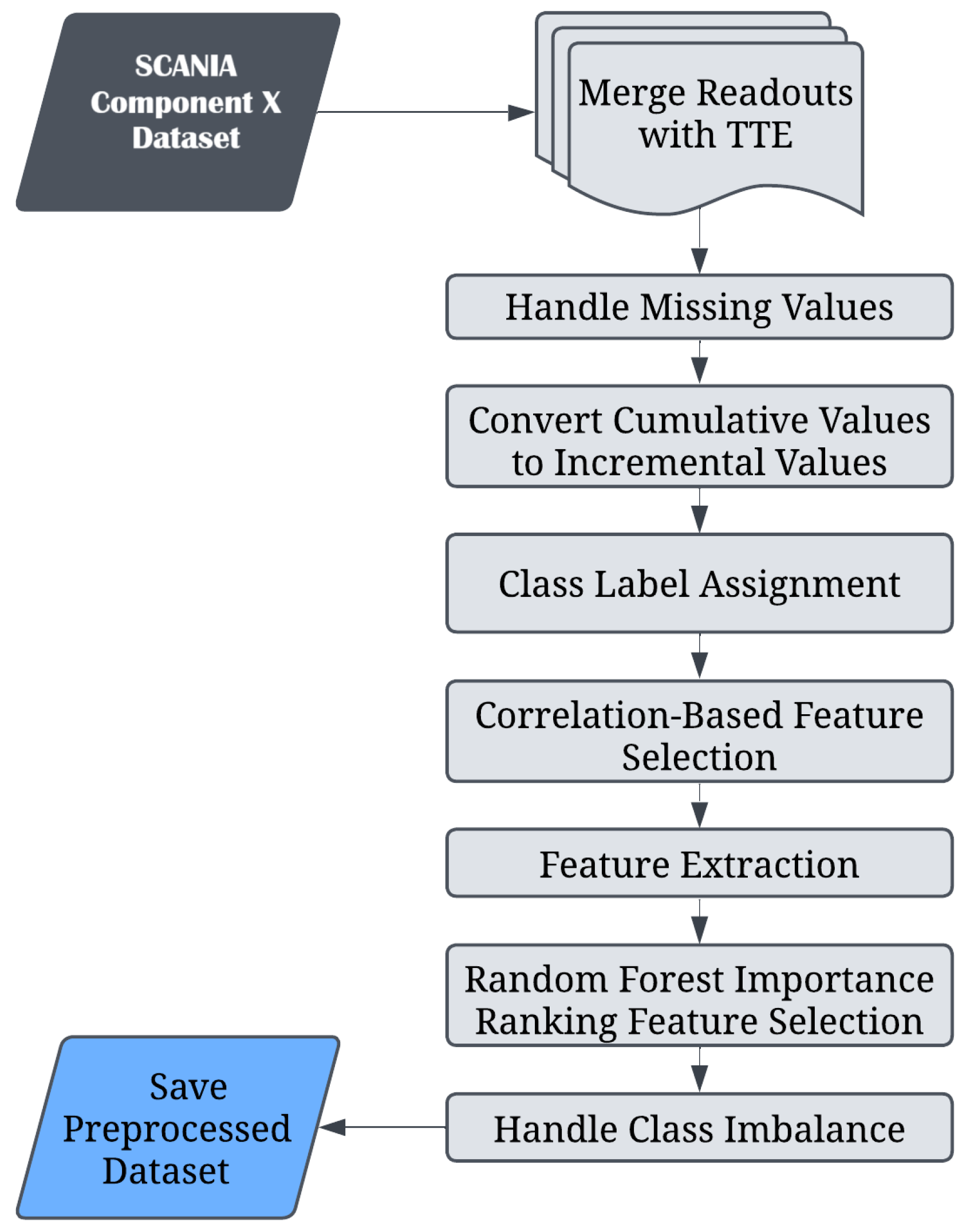
The data preprocessing framework employed in this research is depicted in Figure 3. The initial step involved merging the operational readout data with the corresponding tte data, facilitating subsequent class label conversion. Following this merge, missing values within the datasets were addressed. Initially, linear interpolation was employed to estimate missing values using adjacent data points within each vehicle’s time series. Where gaps persisted post-interpolation, forward filling was utilised to propagate existing data points forward in time.

As previously highlighted, numerical counters within the dataset are cumulative by design and therefore require conversion into incremental values. This conversion facilitates clearer analysis of component progression and degradation over discrete time intervals. Following this, in the training set specifically, class labels were derived by computing the temporal difference (delta) between the “length_of_study_time_step” and original “time_step”. Classification adhered strictly to the criteria established in the validation and test label definitions provided by the dataset creators: class 4 represents a delta interval of 0–6 time steps prior to failure, class 3 represents 6–12, class 2 corresponds to 12–24, class 1 encompasses 24–48, and class 0 denotes intervals exceeding 48 time steps [36]. For vehicles that remained unrepaired throughout the duration of the study (i.e., those marked with in_study_repair = 0), the final 48 time steps of data were intentionally excluded from the analysis, as these measurements were deemed too close to the study’s endpoint to provide reliable contributions to the predictive models.

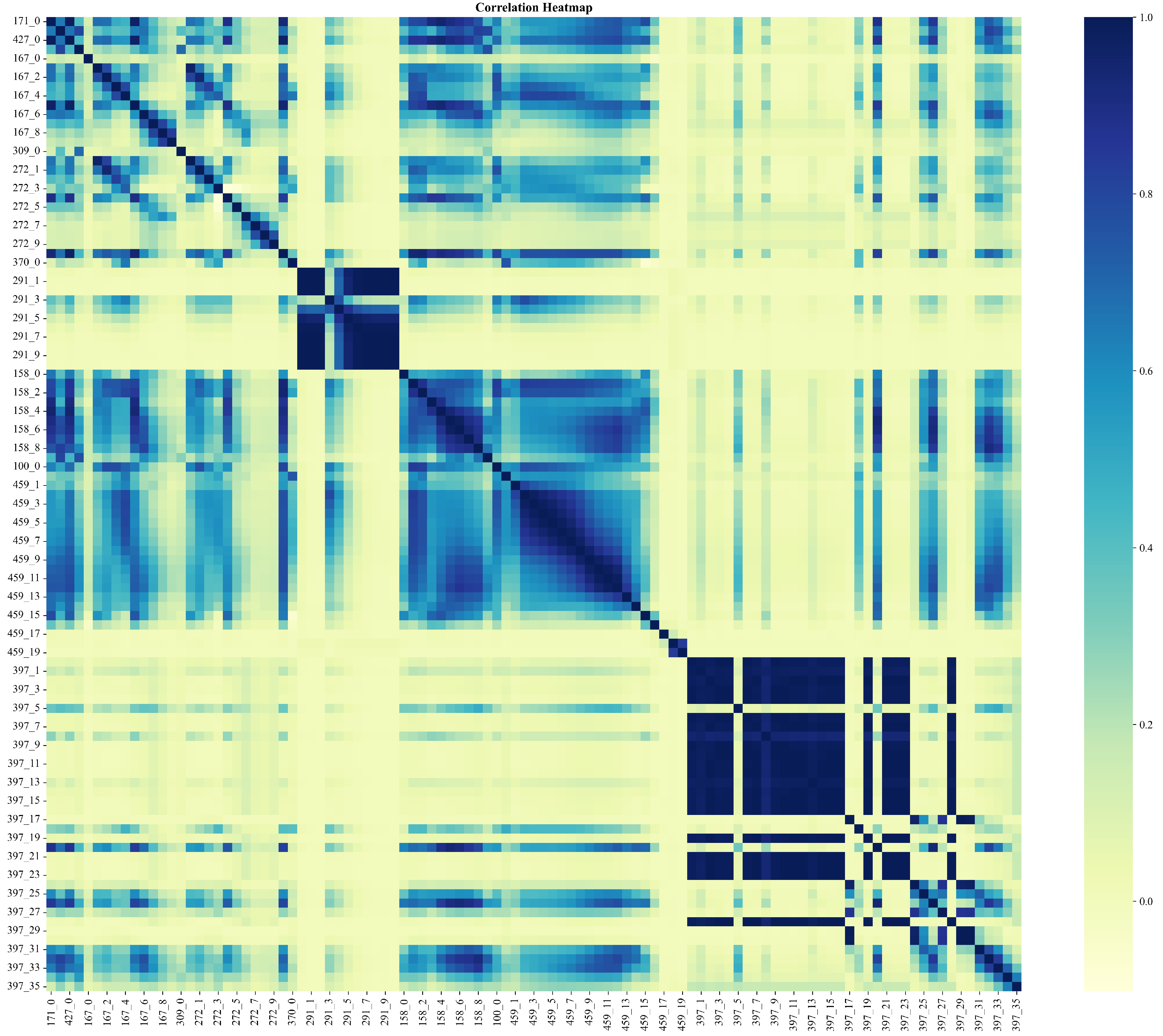
In considering that the original dataset contained 105 features, an analysis of the correlation heatmap, Figure 4, revealed distinct clusters of highly correlated variables, enabling the removal of redundant information. Variables exhibiting correlation coefficients exceeding a threshold of 0.9 were consequently excluded. This procedure reduced the feature dimensionality substantially, yielding a refined dataset comprising 51 unique variables. Given that the initial data were structured as sequential multivariate time series, a transformation into a structured tabular format was essential to facilitate predictive analysis through machine learning algorithms. To achieve this transformation, the tsfresh library was utilised to perform feature extraction via a sliding window approach. Specifically, windows of lengths 4, 8, 16, 32, and 48 time steps were selected to evaluate the influence of temporal resolution on predictive performance. The algorithm implemented for window creation is detailed as follows:

• Sensor readings for each vehicle were arranged chronologically according to their recorded time steps.
• Sequential sliding windows of a defined length were generated, with each new window offset by 4 steps, thereby reducing overlap and computational complexity.
• Each window comprised sensor data uniquely identified by concatenating the vehicle identifier, the end index of the window, and the specified window size.
• Class labels for supervised learning tasks were extracted from the final observation within each window, thereby linking each window directly with the most recent operational state of Component X.

After the feature extraction process, each resultant dataset was annotated with the appropriate class label and corresponding window size, explicitly associating each feature set with its temporal context. Subsequently, the feature sets derived from all specified window sizes were consolidated into a single dataset. To evaluate the relative importance of these newly derived features, a baseline Random Forest model was trained, allowing for the identification of key discriminative features. A subset of the top 100 features was retained for modelling. The final preprocessing stage addressed the inherent class imbalance within the dataset through the adoption of two distinct strategies, designed to identify the most effective approach. The first approach involved downsampling the majority class (class label = 0) to match the combined total number of samples across all minority classes. The alternative method initially reduced the majority class to 20,000 samples before applying the SMOTETomek algorithm, a synthetic oversampling technique combined with undersampling. The rationale behind this two-step approach was primarily computational; by initially reducing the dataset size, the subsequent application of the more computationally intensive SMOTETomek procedure became significantly more manageable.

4. Training and Hyperparameter Optimisation

4.1. Cross-Validation Strategy

To ensure robust and generalisable performance evaluation, a five-fold cross-validation strategy was employed during model training and hyperparameter optimisation. In each iteration, the dataset was divided into five mutually exclusive subsets, with the model trained on four subsets and validated on the remaining one. This process was repeated such that each data point contributed to both training and validation. While stratified k-fold cross-validation is often recommended for classification tasks to preserve class distributions across folds, this study employed standard k-fold cross-validation. The decision was driven by the severe class imbalance in the dataset, particularly the predominance of class 0. In such contexts, stratification can result in minority classes being sparsely represented in some folds, thereby introducing instability in the cost-based scoring metric. Standard k-fold cross-validation mitigated this issue by promoting more consistent exposure to class variation across folds. The choice of five folds reflected a balance between computational efficiency and the stability of performance estimates. Preliminary tests with three folds indicated greater variability in cost evaluation, whereas ten folds significantly increased runtime without yielding meaningful gains in predictive reliability.

4.2. Custom Cost-Based Scoring

A custom scoring function, derived from the SCANIA cost matrix, was implemented to ensure that model evaluation aligns with the practical demands of predictive maintenance. The matrix imposes asymmetric penalties, assigning substantially higher costs to false negatives than to false positives. This design mirrors real-world consequences, where undetected failures can lead to unexpected downtime or pose serious safety risks.

The cost matrix, introduced in [36], is shown in

Table 2. SCANIA misclassification cost matrix.

True\Pred	0	1	2	3	4
0	0	7	8	9	10
1	200	0	7	8	9
2	300	200	0	7	8
3	400	300	200	0	7
4	500	400	300	200	0

. Each entry $C_{n,m}$ represents the penalty incurred for predicting class m when the true class is n.

To integrate this cost function into model selection, a custom scoring routine was defined. During validation, predictions were aggregated at the vehicle level by considering only the final time step for each vehicle. This approach ensured alignment with the operational context of the dataset, where maintenance decisions are based solely on the truck’s final health state. By focusing on the last available readout, the scoring routine maintained consistency with the cost formulation, where penalties are applied only to misclassifications of a vehicle’s final diagnostic label. The total misclassification cost was computed by summing the appropriate penalties from the matrix across all vehicles in the validation fold. This cost was negated and used as the optimisation criterion in GridSearchCV, thereby replacing standard metrics such as accuracy or F1-score. The objective was to identify hyperparameter configurations that minimise overall economic impact, rather than optimise generic predictive metrics.

4.3. Hyperparameter Tuning

Hyperparameters for each model were selected based on their relevance to model complexity and regularisation. The tuning choices are summarised below:

• DT: Only the max_depth parameter was tuned, given the model’s sensitivity to depth and its impact on interpretability and generalisation.
• KNN: The number of neighbours (k) was varied to assess local generalisation performance. Values of $k=3$ and $k=5$ were tested.
• RF: The number of trees (n_estimators) was fixed at 100 to ensure consistency, while max_depth was tuned to manage overfitting and maintain model simplicity.
• SVM: The penalty term C and kernel type were tuned, with a particular focus on the RBF kernel given its effectiveness in capturing non-linear patterns.
• MLP: The size of the hidden layer and the regularisation strength (alpha) were tuned. A single hidden layer was used to limit training time and reduce overfitting risk.
• LightGBM: The number of leaves (num_leaves) was tuned, reflecting the maximum number of nodes in one tree. Other parameters, such as learning rate and boosting type, were kept at their default values.
• XGBoost: The maximum depth (max_depth) of the trees was tuned while keeping the number of estimators fixed. The default learning rate and objective for multi-class classification were used.

Final configurations were selected based on the lowest average cost per vehicle across validation folds.

4.4. Class Imbalance Handling

As already mentioned, the dataset is highly imbalanced, with the majority of samples belonging to the non-failure class (Class 0). This imbalance poses a significant challenge for learning algorithms, as it may lead to models biased towards the majority class while failing to correctly identify critical failure events. To address this issue, three different strategies were employed and compared:

• Downsampling of Class 0: To reduce the dominance of the majority class, Class 0 instances were randomly downsampled to match the size of the minority classes. This method was applied prior to training to ensure a more balanced class distribution in the training set.
• Downsampling + SMOTETomek: This hybrid strategy combines random downsampling of Class 0 with SMOTETomek, a resampling technique that synthesises new minority class instances via SMOTE (Synthetic Minority Over-sampling Technique) and cleans overlapping samples with Tomek links. This approach aimed to balance the dataset more effectively while reducing noise and class overlap.
• Class Weighting: A manually defined class weight scheme was introduced to penalise the misclassification of minority classes more heavily. This approach was applied selectively, as not all models support class weighting and its computational cost can be prohibitive in certain cases. The class weights were set as {0: 1, 1: 10, 2: 20, 3: 30, 4: 40}, aligning with the relative severity of each class label.

4.5. Ensemble Learning: Voting Classifier

To further enhance predictive performance and robustness, an ensemble model was implemented using a hard-voting classifier. The ensemble combined the three best-performing classifiers under the downsampling strategy: SVM, Random Forest, and XGBoost. Each base model was independently trained with hyperparameters optimised according to the cost-sensitive scoring function. Final predictions were determined through majority voting, allowing the ensemble to benefit from the complementary strengths of individual learners while reducing the impact of their respective limitations.

4.6. Baseline Models

To establish reference points for model evaluation, following the approach outlined in [38], two naive baseline models were implemented. The first baseline consistently predicted Class 0, which represents the majority class in the dataset. The second baseline predicted Class 4 for all instances, reflecting the most severe failure class. These baselines served as lower-bound benchmarks for evaluating the effectiveness of trained models under the cost matrix. Although these approaches are not practical for real-world deployment, they highlight the importance of cost-sensitive strategies by demonstrating the substantial penalties associated with misclassification.

5. Results

To evaluate model performance, four primary metrics were used: accuracy, macro-averaged F1-score, total misclassification cost, and average cost per vehicle. Each metric provides a distinct perspective on model performance, particularly in the context of class imbalance and cost sensitivity. The following subsections outline and justify the use of each metric.

5.1. Accuracy

Accuracy quantifies the proportion of correct predictions relative to the total number of predictions. While widely used, accuracy can be misleading in the presence of class imbalance, as it may over-represent the majority class. Consequently, while accuracy is reported for completeness, it is not the primary metric used for model selection.

$$\mathrm{Accuracy}={\displaystyle \frac{TP+TN}{TP+TN+FP+FN}}$$

(1)

where

• TP: True Positives;
• TN: True Negatives;
• FP: False Positives;
• FN: False Negatives.

5.2. Macro F1-Score

The macro-averaged F1-score calculates the harmonic mean of precision and recall independently for each class and then averages the result. This metric is particularly appropriate for this study as it gives equal importance to all failure classes, regardless of their frequency in the dataset. This ensures that the model’s ability to detect rare but costly failures is not overshadowed by its performance on the majority class. It was used alongside cost-based metrics to assess classification performance more holistically.

$$F{1}_i={\displaystyle \frac{2·{\mathrm{Precision}}_i·{\mathrm{Recall}}_i}{{\mathrm{Precision}}_i+{\mathrm{Recall}}_i}}$$

(2)

$$\mathrm{Macro}\mathrm{F}1={\displaystyle \frac{1}{C}}\sum _{i=1}^{C}F{1}_i$$

(3)

where C is the total number of classes.

5.3. Total Misclassification Cost

Total cost directly captures the business-critical objective of minimising failure-related costs. Unlike generic classification metrics, it incorporates the asymmetric cost structure defined by the dataset providers. Let $y_i$ be the true class and ${\widehat{y}}_i$ the predicted class for vehicle i. Then,

$$\mathrm{Total}\mathrm{Cost}=\sum _{i=1}^N\mathrm{Cost}(y_i,{\widehat{y}}_i)$$

(4)

where $\mathrm{Cost}(y_i,{\widehat{y}}_i)$ is retrieved from the misclassification cost matrix in Table 2. This metric was used as the primary objective in model selection, particularly during hyperparameter tuning, as it aligns directly with the goal of finding the cost-efficient model.

5.4. Average Cost per Vehicle

To fairly compare model performance at the vehicle level, total cost is normalised by the number of unique vehicle identifiers:

$$\mathrm{Avg}.\mathrm{Cost}\mathrm{per}\mathrm{Vehicle}={\displaystyle \frac{\mathrm{Total}\mathrm{Cost}}{N_{\mathrm{vehicles}}}}$$

(5)

This metric offers a per-unit cost perspective that accounts for class distribution across different vehicles and avoids the distortion that can arise from multiple readouts per vehicle. It serves as a complementary indicator to total cost and is also used to compare ensemble and baseline models.

5.5. Performance of Individual Models

Table 3. Best hyperparameters for each model under the downsampling strategy.

Model	Best Parameters
Decision Tree	max_depth = 10
K-Nearest Neighbour	n_neighbors = 3
Random Forest	n_estimators = 100, max_depth = 10
Support Vector Machine	kernel = rbf, C = 1
Multi-Layer Perceptron	hidden_layer_sizes = (50), alpha = 0.0001
LightGBM	num_leaves = 31, n_estimators = 100
XGBoost	n_estimators = 100, max_depth = 3

presents the optimal hyperparameters for each model trained under the downsampling strategy. Following hyperparameter tuning, all models were evaluated on the test set, and the corresponding performance results are summarised in

Table 4. Test set performance of models trained with downsampling.

Model	Accuracy	F1 (Macro)	Total Cost	Avg. Cost per Vehicle
DT	0.90	0.20	44,587	8.97
KNN	0.74	0.18	48,373	9.74
RF	0.97	0.20	42,684	8.59
SVM	0.97	0.20	43,195	8.69
MLP	0.89	0.19	46,033	9.27
LightGBM	0.90	0.19	46,282	9.32
XGBoost	0.93	0.19	45,055	9.07

.

Among the evaluated models, RF and SVM achieved the highest accuracy (0.97) and tied for the best F1-score (0.20). Notably, RF also yielded the lowest total misclassification cost (42,684) and the lowest average cost per vehicle (8.59), indicating strong cost-efficiency and predictive robustness. DT and LightGBM achieved moderate accuracy (0.90) but incurred slightly higher average costs compared to RF and SVM. KNN recorded the lowest overall performance across all metrics, with an accuracy of 0.74 and the highest average cost per vehicle (9.74), highlighting its sensitivity to high-dimensional data in the predictive maintenance context. Although MLP achieved reasonable accuracy (0.89), it underperformed in terms of cost metrics, likely due to its susceptibility to data imbalance and sensitivity to hyperparameter tuning. XGBoost provided a good balance between predictive performance and cost, achieving 0.93 accuracy with an average cost of 9.07. Overall, downsampling proved effective in enabling balanced performance across most models, with ensemble-based methods such as RF and XGBoost outperforming simpler learners in cost-aware evaluations.

5.6. Model Performance: Downsampling + SMOTETomek

Table 5. Best hyperparameters for each model under the downsampling + SMOTETomek strategy.

Model	Best Parameters
Decision Tree	max_depth = 10
K-Nearest Neighbour	n_neighbors = 5
Random Forest	n_estimators = 100, max_depth = 10
Support Vector Machine	kernel = rbf, C = 1
Multi-Layer Perceptron	hidden_layer_sizes = (50), alpha = 0.0001
LightGBM	num_leaves = 31, n_estimators = 100
XGBoost	n_estimators = 100, max_depth = 3

presents the optimal hyperparameters identified for each model under the downsampling + SMOTETomek strategy. Performance on the test set is summarised in

Table 6. Test set performance of models trained with Downsampling + SMOTETomek).

Model	Accuracy	F1 (Macro)	Total Cost	Avg. Cost per Vehicle
DT	0.32	0.11	52,274	10.52
KNN	0.32	0.11	53,805	10.83
RF	0.56	0.15	52,208	10.51
SVM	0.59	0.16	52,208	10.51
MLP	0.49	0.14	50,127	10.09
LightGBM	0.60	0.16	51,998	10.47
XGBoost	0.52	0.15	53,543	10.78

.

Compared to the downsampling-only approach, the downsampling + SMOTETomek strategy resulted in generally poorer predictive performance across all models. Notably, DT and KNN recorded the lowest accuracy (0.32) and F1-score (0.11), with KNN also incurring the highest average cost per vehicle (10.83). While SVM, LightGBM, and RF showed slightly better performance, their metrics still lagged behind their counterparts trained using simple downsampling. For instance, RF achieved 0.56 accuracy and 0.15 F1 under SMOTETomek, compared to 0.97 accuracy and 0.20 F1 under downsampling. Similarly, SVM’s accuracy dropped from 0.97 to 0.59, and its average cost increased from 8.69 to 10.51. Interestingly, LightGBM exhibited the strongest performance under SMOTETomek, with 0.60 accuracy, 0.16 macro F1, and the lowest average cost (10.47) among all models in this group. However, this still fell short of its performance under downsampling (0.90 accuracy, 0.19 macro F1, and 9.32 avg. cost).

6. Discussion

This section discusses the empirical findings of the study by addressing the research questions posed in the Introduction section. This discussion is grounded in the results presented in the previous section, with a focus on evaluating predictive performance, imbalance handling strategies, and model cost-efficiency in the context of predictive maintenance for Component X.

RQ1: To what extent can machine learning models accurately predict failures of Component X in a cost-sensitive setting? The predictive results indicate that failures of Component X can be detected with reasonable accuracy using classical machine learning models, particularly under a cost-aware and class-imbalanced setting. When trained using the downsampling strategy, SVM and RF achieved the highest test accuracy (0.97) and competitive macro F1-scores (0.20), outperforming other models in both predictive accuracy and cost-efficiency. However, confusion matrix analysis, Figure 5, reveals a critical limitation of these models: despite overall high accuracy, both RF and SVM exhibit poor recall for minority classes (i.e., failure classes 1–4). This reflects a common problem in class-imbalanced settings, where models tend to prioritise the dominant class (Class 0) to optimise global accuracy [40], often at the expense of minority class detection. For example, the RF model predicted nearly all samples as Class 0, correctly classifying only two minority-class instances out of over 3700. This suggests persistent class imbalance issues or model bias toward the dominant class, contributing to low macro F1-scores. This could be addressed with loss reweighting to prioritize minority classes, focal loss to focus on hard-to-classify samples, or temporal deep learning models like Long Short-Term Memory (LSTM) networks to better capture time-series dependencies.

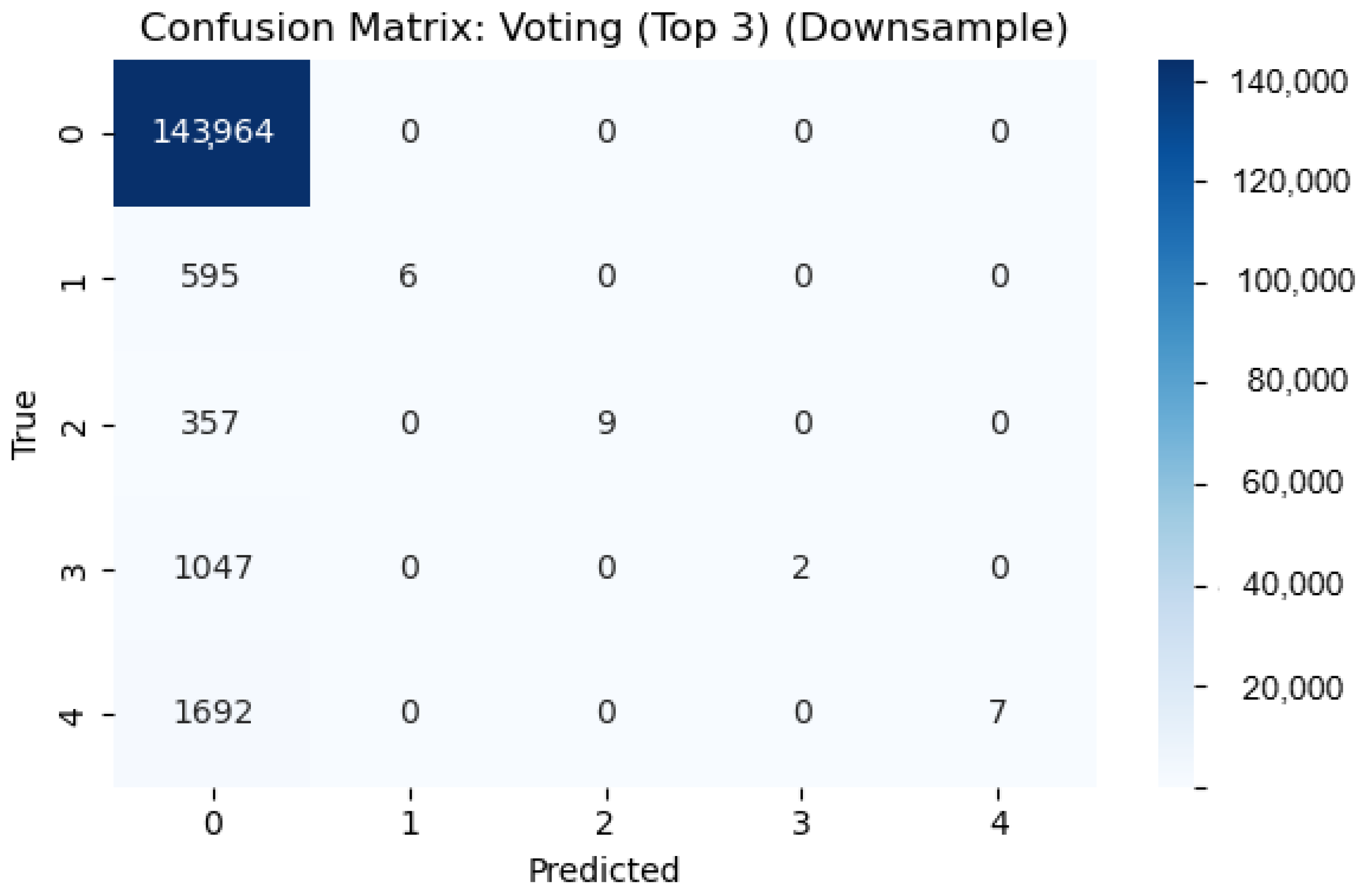
To address this, an ensemble model was proposed using a hard-voting classifier that combined the top three performing models under the downsampling strategy: SVM, RF, and XGBoost. As shown in Figure 6, the voting classifier exhibited improved minority class coverage, correctly identifying several instances in each failure class (e.g., 6 in Class 1, 9 in Class 2, and 7 in Class 4). Although the improvements in macro F1-score (0.21) and accuracy (0.98) appear modest, the voting classifier delivered the lowest total misclassification cost (41,600) and lowest average cost per vehicle (8.37)—outperforming even the individual RF model.

This suggests that while high classification accuracy can be achieved, such results may obscure imbalanced class performance. Cost-aware evaluation metrics and ensemble learning techniques are thus crucial in developing models that perform robustly across all failure modes in real-world predictive maintenance tasks.

RQ2: Which class imbalance handling strategy yields better overall performance? This study addressed the class imbalance problem using three strategies: (i) downsampling only, (ii) downsampling combined with SMOTETomek, and (iii) customised class weighting. As the third strategy was applied selectively to only a few models, it is excluded from the comparative performance discussion. When comparing the first two strategies, the results clearly demonstrate that downsampling alone consistently outperformed the combined approach. Across nearly all models, both accuracy and macro F1-scores were notably higher under downsampling, and total misclassification costs were consistently lower. For example, RF achieved an accuracy of 0.97 with a total cost of 42,684 under downsampling, while its performance deteriorated to 0.56 accuracy and 52,208 in cost when trained with SMOTETomek. A similar trend was observed for SVM, LightGBM, and XGBoost. Even the best-performing model under the SMOTETomek strategy, LightGBM, incurred a higher misclassification cost (51,998) than all top-performing models trained with downsampling. These findings suggest that although SMOTETomek is theoretically intended to improve class balance by combining over- and under-sampling, it may introduce synthetic noise or distort the original data distribution, ultimately reducing model generalisability. This effect appears particularly pronounced for high-capacity models such as SVM and RF. Additionally, the introduction of synthetic minority samples may adversely impact algorithms that are sensitive to feature space geometry, including KNN and MLP.

RQ3: Which predictive model provides the optimal trade-off between classification performance and misclassification cost? Figure 7 illustrates the average misclassification cost per vehicle for all models. The two models that achieved a lower cost than the baseline that predicts all samples as Class 0 (average cost = 8.62) were the following: Voting Classifier (downsampling only) and RF (downsampling only) (8.37 and 8.59, respectively). This finding is significant, as these are the only models that outperformed both baseline models, confirming their suitability for cost-sensitive deployment scenarios. Conversely, none of the models trained with Downsampling + SMOTETomek were able to outperform even the second baseline, a model that predicts all samples as Class 4 (average cost = 9.88). For instance, the best-performing SMOTETomek model (LightGBM) recorded an average cost of 10.47, indicating that despite attempts to improve class balance, this strategy compromised cost-effectiveness. Among all approaches, the Voting Classifier offered the most favourable trade-off, balancing modest gains in predictive performance with superior cost-efficiency. By combining top-performing classifiers (SVM, RF, XGBoost), it effectively reduced the misclassification impact across all failure classes, reinforcing the value of ensemble learning in cost-critical applications. These findings highlight a critical trade-off: models optimised purely for predictive performance may still be suboptimal in cost-sensitive settings, and vice versa. The results reaffirm that both metrics must be evaluated jointly when selecting models for real-world PdM applications.

To further contextualise our findings, it is worth comparing the performance of the classical machine learning models employed in this study with deep learning-based approaches, such as Long Short-Term Memory (LSTM) networks or Convolutional Neural Networks (CNNs), which are often used for predictive maintenance tasks involving time-series or high-dimensional data. While our results demonstrate that classical models such as SVM, RF, and the Voting Classifier achieve high accuracy (up to 0.98) and cost-efficiency (lowest average cost of 8.37 per vehicle) under a downsampling strategy, they struggle with minority class recall due to class imbalance. Deep learning models, particularly LSTMs, could potentially address this limitation by capturing temporal dependencies in the failure data of Component X, which may improve the detection of rare failure events (Classes 1–4). However, deep learning approaches typically require larger datasets and higher computational resources, which may not be feasible in cost-sensitive settings. Additionally, their performance can be sensitive to hyperparameter tuning and may not guarantee superior results compared to our ensemble approach, which uses the strengths of multiple classical models to achieve robust cost-performance trade-offs.

Limitations

This study presents several limitations that warrant consideration. Firstly, despite the application of a downsampling strategy to mitigate class imbalance, the trained models still exhibited poor recall for minority failure classes. This limited their ability to detect rare yet operationally critical events, as evidenced by the confusion matrices. Secondly, the reliance on hand-crafted features extracted from sliding windows may have constrained the models’ ability to learn nuanced temporal relationships in the sensor data. This limitation is particularly relevant for failure progression patterns that evolve gradually over time. The scope of algorithm selection was restricted to a set of well-established classical classifiers, potentially overlooking more adaptive or domain-specific modelling paradigms. The generalisability of the proposed approach remains to be established, as all experiments were conducted exclusively on the SCANIA Component X dataset. While this dataset reflects realistic industrial conditions, further testing on other systems is necessary to validate the wider applicability of the findings.

7. Conclusions

This research presented a comprehensive, cost-sensitive machine learning pipeline for the failure prediction of Component X in heavy-duty trucks. This study explored seven supervised learning models, ranging from interpretable algorithms such as DT to advanced ensemble methods like XGBoost and LightGBM, applied to features extracted from multivariate time-series data via a sliding window and tsfresh-based pipeline. To address the severe class imbalance in the dataset, three strategies were investigated: (i) downsampling of the majority class, (ii) downsampling combined with SMOTETomek, and (iii) custom class weighting. Evaluation was performed using the accuracy, macro F1-score, and SCANIA-specific misclassification cost function. The results demonstrate that the downsampling strategy outperformed the alternatives in both predictive and cost-efficiency terms. The best-performing model, RF, trained under the downsampling strategy, achieved an accuracy of 0.97 and the lowest average cost per vehicle (8.59). An ensemble model, constructed via hard voting across SVM, Random Forest, and XGBoost, further improved robustness and achieved the lowest total cost (41,600). These findings indicate that, under certain conditions, classical machine learning models, when paired with appropriate preprocessing and imbalance-handling techniques, can offer cost performance that is comparable to more complex deep learning methods previously applied to the same dataset, while presenting potential benefits in terms of lower computational demands and greater interpretability.

8. Future Work

Future research could extend this work in several directions. A key priority is to explore additional strategies for mitigating class imbalance beyond downsampling and resampling. Approaches such as dynamic class reweighting, cost-sensitive loss functions, or hybrid resampling techniques may further enhance minority class detection. Temporal modelling also presents a promising avenue: integrating sequential architectures such as Long Short-Term Memory (LSTM), Gated Recurrent Units (GRUs), or Transformer-based networks could capture richer temporal dependencies and improve predictive performance in time-series contexts. Expanding the ensemble framework to include soft voting, stacking, or explicitly cost-aware ensemble designs could yield more balanced performance in high-stakes settings. Although this research focused on classification, future work could revisit Remaining Useful Life (RUL) estimation using survival analysis or time-to-event models, incorporating cost-sensitive objectives. Transitioning the proposed system into a real-time deployment environment would offer insight into its operational viability, including model latency, interpretability, and performance stability under live conditions. This study’s focus on SCANIA Component X limits its generalizability to other industrial contexts, necessitating further research to explore scalability across diverse applications. Future work should investigate the adaptability of the findings in varied industrial settings to enhance broader applicability.