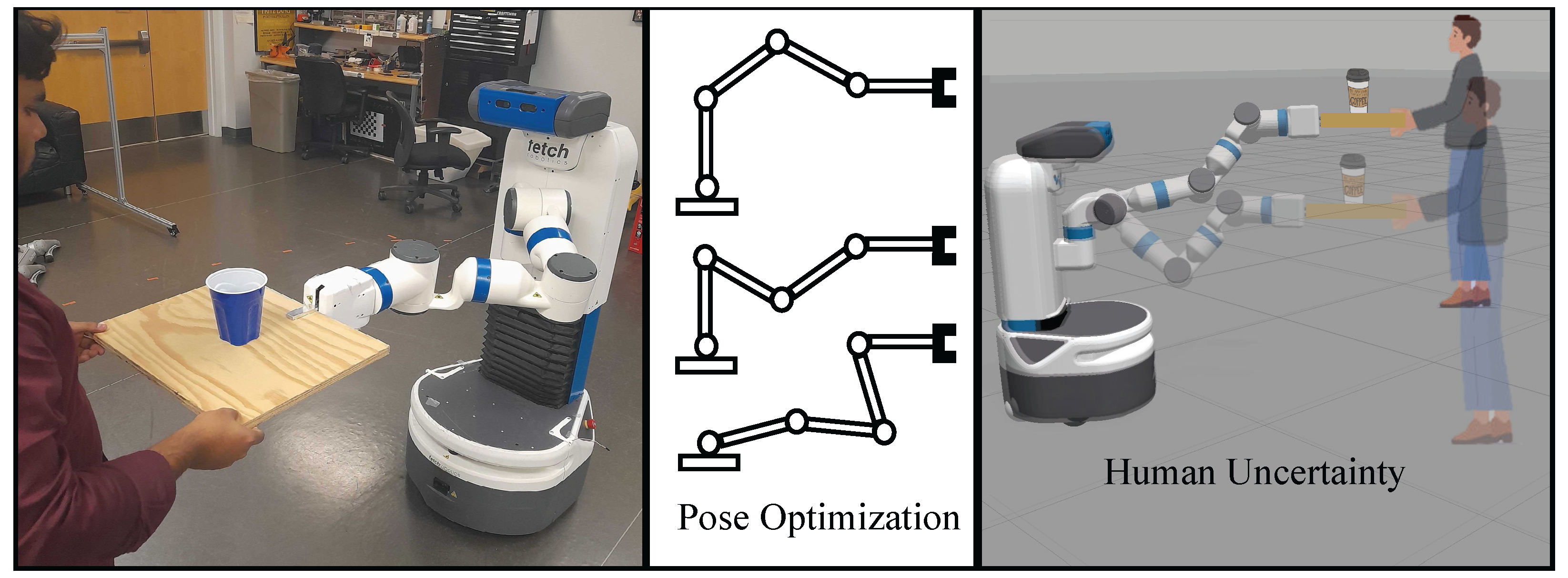
DARC: Disturbance-Aware Redundant Control for Human–Robot Co-Transportation

Abstract

This paper introduces Disturbance-Aware Redundant Control (DARC), a control framework addressing the challenge of human–robot co-transportation under disturbances. Our method integrates a disturbance-aware Model Predictive Control (MPC) framework with a proactive pose optimization mechanism. The robotic system, comprising a mobile base and a manipulator arm, compensates for uncertain human behaviors and internal actuation noise through a two-step iterative process. At each planning horizon, a candidate set of feasible joint configurations is generated using a Conditional Variational Autoencoder (CVAE). From this set, one configuration is selected by minimizing an estimated control cost computed via a disturbance-aware Discrete Algebraic Riccati Equation (DARE), which also provides the optimal control inputs for both the mobile base and the manipulator arm. We derive the disturbance-aware DARE and validate DARC with simulated experiments with a Fetch robot. Evaluations across various trajectories and disturbance levels demonstrate that our proposed DARC framework outperforms baseline algorithms that lack disturbance modeling, pose optimization, or both.

1. Introduction

Human–robot collaboration is an emerging topic in research that helps to reduce humans’ physical and cognitive workloads in various applications. For example, in industrial applications, collaborative robots are often used to perform repetitive tasks that enhance productivity and reduce human effort [1,2]. In such scenarios, robots generally operate behind safety fences, with physical separation from humans, to ensure safety [3]. Moreover, when humans and robots share the same workspace, the robots must be aware of human movements to ensure safety and achieve task goals [4]. This is important in both industrial and non-industrial settings. The application in non-industrial settings includes supporting elderly people with daily activities [5] and providing navigation assistance to individuals [6]. These applications require high-level planning with low-level control of the robot to achieve increased performance while maintaining safety. Increased performance refers to comparison with the performance level of either humans or robots operating independently [7].

Among these diverse applications, the co-transportation of objects by a human with a mobile manipulator (i.e., a robotic arm mounted on a mobile base) is a common scenario [8], as illustrated in Figure 1. In human–robot co-transportation tasks, there are challenges in ensuring safe and efficient performance, especially when subjected to disturbances [9,10]. These disturbances include unpredictable human behavior, hardware imperfections such as sensor noise or actuator inaccuracies, etc. Even if the task has a predefined nominal path, humans often deviate from it due to fatigue, personal preferences, or external influences [11,12]. These deviations need to be compensated for by the robot to achieve the task goals. For a mobile manipulator, such adaptation toward disturbances is complex, as the robotic arm must dynamically reconfigure its joint angles to adapt to the human.

The high-level planning of a mobile manipulator highly relies on the Model Predictive Control (MPC) framework, which has the predictive capabilities to enhance collaborative task performance [13]. However, this framework may lead to singularities or semi-singularities where the arm loses degrees of freedom or becomes stuck [14]. To address (semi-)singularities, proactive pose optimization can be implemented by exploiting the manipulator’s kinematic redundancy [15,16]. Yet, limited existing works consider the integration of MPC and pose optimization, and they are not directly applicable to the co-transportation task considered in this paper [17,18]. Furthermore, the complexity rises in a mobile manipulator compared to a fixed-base robotic arm. Although using a mobile manipulator extends the system’s workspace and maneuverability, such flexibility challenges the simultaneous coordination of the base’s mobility with the arm’s joint angle velocities [19].

To address these challenges, this work (a preprint of this paper is available in [20]) proposes a DARC framework by combining a disturbance-aware Model Predictive Control strategy as a high-level planner with a pose optimization mechanism at the low-level control. The MPC component plays the role of coordinating the movements of the mobile base and robotic arm by estimating the effects of disturbances on tracking accuracy and energy consumption. At the low-level control, we use a pose optimization mechanism that dynamically adjusts the robot’s joint angles to compensate for disturbances. This also helps avoid singularities and enhances tracking accuracy under disturbances. This two-step interactive process, integrating the predictive capability of MPC and the proactive control of the robot with pose optimization, helps to reduce control effort and improve energy efficiency and tracking performance.  

Statement of Contribution: The main contributions of this paper are as follows:

• We formulate a high-level Model Predictive Control (MPC) planner problem that incorporates disturbances along with a low-level pose optimization mechanism and the robot’s whole-body kinematics. We propose a two-step iterative optimization approach to holistically solve the high-level and low-level problems.
• For the high-level MPC problem, we estimate control costs under disturbances and generate optimal control inputs. The initial state of the MPC controller depends on the low-level pose optimization.
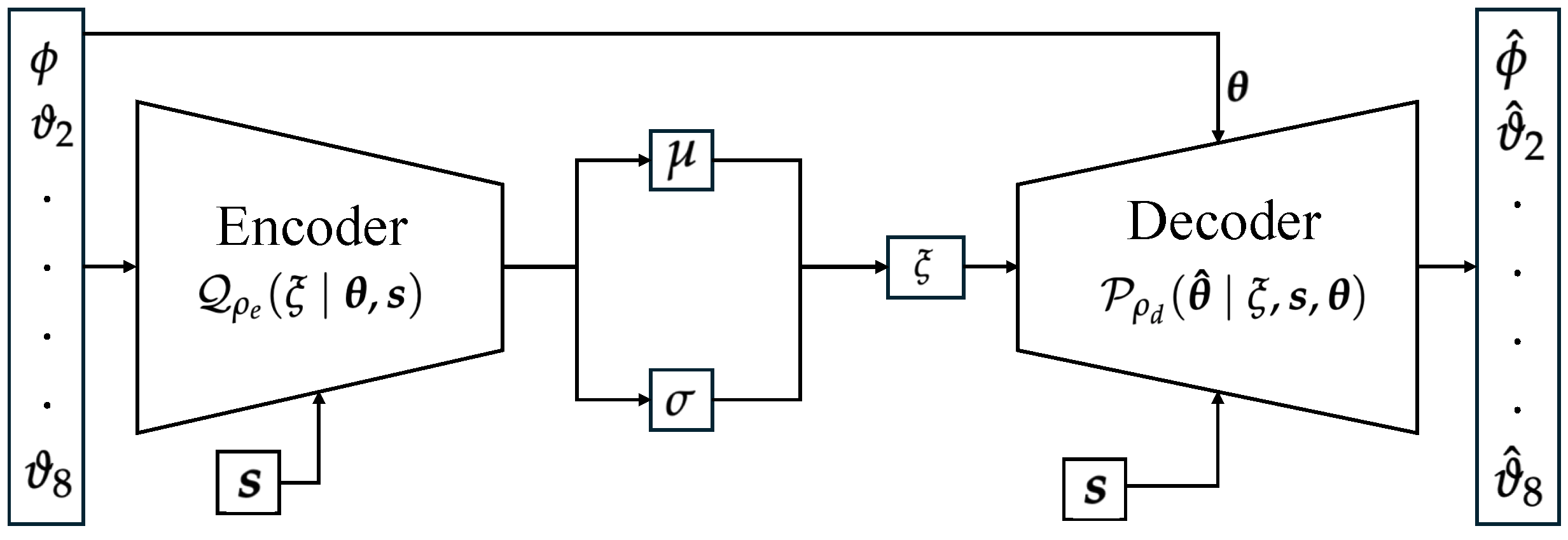
• For the low-level pose optimization, we optimize the robot’s pose selected from a joint configuration set generated using Conditional Variational Autoencoder (CVAE). The selection criteria are informed by the expected cost of the high-level MPC.
• We provide theoretical derivations and simulated experiments with a Fetch mobile manipulator to validate the DARC framework. Quantitative comparisons highlight the advantages of our method over different baselines.

2. Literature Review

Human–robot collaboration can be broadly classified into four levels based on their interaction modes: (i) physical separation (No Coexistence), (ii) shared space with no shared goals (Coexistence), (iii) shared goals in shared space (Cooperation), and (iv) simultaneous work on a shared object in shared space (Collaboration) [21,22]. Co-transportation work falls into level (iv) as the human and the robot carry the same object in the same environment.

To enhance the performance of such collaborative tasks while ensuring safety by adapting to humans, integrating model-based control and reinforcement learning has been explored. Recent works use model-based reinforcement learning to assist humans in target activities [23], perform wood sawing and surface polishing [24], and execute Gaussian Process MPC in collaborative assembly tasks [13]. Furthermore, studies consider robust variable admittance control with unknown payload [25], sampling-based MPC for task and motion planning [26], and combined task/joint-space constraint handling [27]. Co-manipulation and transportation tasks are also addressed by considering whole-body kinematics of mobile manipulators [28,29,30] or employing human–humanoid collaboration strategies [31,32,33] to reduce human workload. While reinforcement learning methods are effective for handling unmodeled human uncertainties, they often lack transparency and rigorous guarantees of performance. For such issues, the control-theoretic framework is provided by robust MPC for addressing uncertainties, ensuring strict safety [34], adhering to physical constraints [35], and accommodating parameter variations [36]. However, these approaches do not integrate the disturbance-aware MPC formulation with pose optimization to enhance the overall performance further. This is one of the main differences from the problem addressed in our proposed framework. Additionally, they usually do not embed the disturbance component in the problem formulation itself; rather, they include it in the robot dynamics.

The idea of pose optimization is closely related to redundancy resolution, where multiple joint configurations can achieve a desired end-effector pose [16,37]. Redundancy resolution is one of the most important parts in controlling high-degree-of-freedom robotic systems, particularly for end-effector manipulation. Such kinematic redundancy helps to avoid singularities [38], improves dexterity in confined workspaces [39], and enhances precision under dynamic conditions [40]. Recent research has explored diverse methodologies to address these objectives—for instance, employing Monte Carlo tree search to optimize redundant configurations [41], introducing a sampling-based approach to navigate complex constraint spaces [42], and leveraging stiffness modeling to refine pose selection for task-specific compliance [43]. In soft robotics, [44] demonstrated redundancy resolution for continuum manipulators by adapting poses to flexible forms. Additionally, many researchers have used learning methods for redundant manipulators. These include utilizing the proximal policy optimization algorithm [45], deep deterministic policy gradient algorithm [46], and deep reinforcement learning [47]. In general, these works highlight the adaptability of pose optimization in overcoming environmental and operational constraints. Although pose optimization has been investigated in many scenarios, these seldom account for disturbances [48]. In contrast to prior approaches, our formulation redefines pose optimization by coupling it with a disturbance-aware MPC framework. This strategy helps to select poses that not only satisfy kinematic goals but also minimize the impact of disturbances.

3. Preliminaries and Problem Formulation

In this section, we first define how disturbances impact the co-transportation process in terms of a nominal trajectory for the human and robot to complete the task. Next, we present the kinematic model of a mobile manipulator’s end-effector, where we integrate the kinematics of its mobile base and arm. Finally, we formulate an MPC problem that incorporates pose optimization to address disturbances effectively.

Notations: Let $I_r$ be the $r\times r$ identity matrix and $\mathrm{diag}\{a_1,\dots ,a_r\}$ be a diagonal matrix whose entries are $a_1,\dots ,a_r$. For any vector x, let ${\parallel x\parallel }_2$ be the Euclidean norm. If M is a square matrix, $\mathrm{Tr}\left(M\right)$ is the trace. Additionally, $M\succ 0$ ($M⪰0$) denotes that M is positive (semi-)definite We define ${\parallel x\parallel }_M^2=x^{\top }Mx$.

3.1. Trajectory with External Human Disturbances

Consider the co-transportation task illustrated in Figure 1, where a human and a mobile manipulator jointly move an object. Let

$$\mathit{r}\left(k\right)={\left[r_x\left(k\right),r_y\left(k\right),r_z\left(k\right),r_{\alpha }\left(k\right),r_{\beta }\left(k\right),r_{\gamma }\left(k\right)\right]}^{\top }\in {\mathbb{R}}^6$$

be the manipulator’s end-effector pose, where $(r_x,r_y,r_z)$ denotes the Cartesian position and $(r_{\alpha },r_{\beta },r_{\gamma })$ the orientation in Euler angles, respectively. We define this pose over a finite horizon $k=0,1,\dots ,H$, where H is the planning horizon. To account for external human disturbances, we incorporate a disturbance term $\varpi \left(\tau \right)$ in the trajectory:

$$\mathit{r}\left(k\right)=\tilde{\mathit{r}}\left(k\right)+D\sum _{\tau =0}^k\varpi \left(\tau \right),$$

(1)

where $\tilde{\mathit{r}}\left(k\right)\in {\mathbb{R}}^6$ is a nominal trajectory. If we assume that the task has a desired trajectory, this $\tilde{\mathit{r}}\left(k\right)$ can be treated as known to the human and the robot. Otherwise, we may consider trajectory prediction of $\tilde{\mathit{r}}\left(k\right)$ by the robot based on human behaviors. In existing works, such trajectory prediction can be achieved using geometry-based curve fitting [49], utility function frameworks [50], or learning methods like recurrent neural networks [51,52], LSTM [53,54,55]. We use LSTM (the detailed implementation will be described in the Appendix A) because it can capture temporal dependencies in sequential data. This makes it beneficial in predicting the continuous, non-linear evolution of human movement. The term $\varpi \left(\tau \right)$ represents the disturbance due to human movement, modeled as a Gaussian distribution—i.e., $\varpi \left(\tau \right)\sim \mathcal{N}({\alpha }_{\varpi },{\Sigma }_{\varpi })$ in the $x,y,$ and z directions where $\tau$ denotes the time step. Here, ${\alpha }_{\varpi }\in {\mathbb{R}}^3$ is the non-zero-mean and ${\Sigma }_{\varpi }\in {\mathbb{R}}^{3\times 3}$ is the covariance matrix that captures individual variations or preferences of the human collaborator. $D\in {\mathbb{R}}^{6\times 3}$ is a matrix that maps $\varpi \left(\tau \right)$ into the $6D$ pose space. To focus on the translational disturbances caused by the human, we assume the orientation $(r_{\alpha },r_{\beta },r_{\gamma })$ remains unaffected by these disturbances. This is because the orientation is co-determined by the robot and the human. Thus, the disturbance towards orientation is not necessarily impacted only by the human, and the robot can compensate for this. Thus, we define $D={\left[\begin{array}{cc}{I}_3& {\mathbf{0}}_{3\times 3}\end{array}\right]}^{\top }$.

3.2. End-Effector Kinematics

We illustrate the modeling details using a Fetch Mobile Manipulator [56], as we used this robot for experiments. The Fetch robot has a differential-drive mobile base and a 7-DOF robotic arm. In the following, we consider simplified kinematics, focusing on velocity inputs.

Note that our proposed framework is applicable to either a dynamic or a kinematic model of the end-effector of any kind of mobile manipulator. A dynamic model with torque control requires the use of accurate inertial parameters, the modelling of non-linear Coriolis and gravity terms, and the capturing of friction and actuator dynamics. When using dynamic models instead of kinematic models, the computational and implementation complexity might increase, but the process remains unchanged. Additionally, the approach can be easily generalized to other types of mobile manipulators, such as robots with an omnidirectional base and a robotic arm mounted on top. For this, we only need to modify the corresponding kinematics equations accordingly.

Mobile Base. The kinematics model of the mobile base of the Fetch Mobile Manipulator can be approximated using a standard differential-drive model in the inertial frame (Figure 2a). Let

$${\mathit{s}}_{\mathrm{base}}\left(k\right)={\left[\begin{array}{c}{x}_{\mathrm{base}}\left(k\right)y_{\mathrm{base}}\left(k\right)\varphi \left(k\right)\end{array}\right]}^{\top }\in {\mathbb{R}}^3$$

be the pose of the base. This has Cartesian coordinates $(x_{\mathrm{base}},y_{\mathrm{base}})$ in the inertial frame and heading angle $\varphi$. The state update of $s_{\mathrm{base}}$ from step k to $k+1$ is given by

$${\mathit{s}}_{\mathrm{base}}(k+1)={\mathit{s}}_{\mathrm{base}}\left(k\right)+\Delta t\left[\begin{array}{cc}cos\left(\varphi \right(k\left)\right)& 0\\ sin\left(\varphi \right(k\left)\right)& 0\\ 0& 1\end{array}\right]{\mathit{u}}_{\mathrm{base}}\left(k\right),$$

(2)

where

$${\mathit{u}}_{\mathrm{base}}\left(k\right)={\left[\begin{array}{c}v\left(k\right)\dot{\varphi }\left(k\right)\end{array}\right]}^{\top }\in {\mathbb{R}}^2$$

where the base’s linear velocity is v and the angular velocity is $\dot{\varphi }$ at time k. We denote the time interval as $\mathsf{\Delta }t$. Here, $(v,\dot{\varphi })$ are in the robot’s body frame $\mathsf{\Xi }$, which translates and rotates with the base.

Robotic Manipulator. Fetch robot incorporates a 7-DOF manipulator mounted on top of its base. We denote each joint angle as ${\vartheta }_i$, where $i\in \{2,\dots ,8\}$ represent seven joint angles. In addition, we include the base’s heading angle $\varphi$ as an extra DOF that yields an 8-DOF system as illustrated in Figure 2b. This helps to merge the kinematics of the mobile base and the manipulator by enabling the transformation of the end-effector’s pose in the robot body frame from the inertial frame without any rotation and vice versa. Additionally, it allows the incorporation of the heading angle $\varphi$ into the pose optimization along with the arm’s joint angles. Let

$$\mathit{\theta }={[\varphi ,{\vartheta }_2,\dots ,{\vartheta }_8]}^{\top }\in {\mathbb{R}}^8$$

combine the base’s heading angle and the arm’s seven joint angles. We denote the corresponding angular velocities by

$$\mathit{\omega }={[\dot{\varphi },{\dot{\vartheta }}_2,\dots ,{\dot{\vartheta }}_8]}^{\top }\in {\mathbb{R}}^8.$$

Let $s_{\mathrm{arm}}$ be the end-effector pose in the body frame $\mathsf{\Xi }$. Specifically,

$${\mathit{s}}_{\mathrm{arm}}=\left[\begin{array}{c}{p}_{\mathrm{arm}}\\ {\psi }_{\mathrm{arm}}\end{array}\right]\in {\mathbb{R}}^6,$$

where $p_{\mathrm{arm}}\in {\mathbb{R}}^3$ denotes the Cartesian position of the end-effector in $\mathsf{\Xi }$ frame, and ${\psi }_{\mathrm{arm}}\in {\mathbb{R}}^3$ represents the orientation in Euler angles in the same frame. Note that our use of Euler angles is primarily for simplicity, although we are aware that Euler angles may potentially lead to singularities [57]. In our application, the target end-effector orientation is maintained horizontally relative to the ground, which helps mitigate the issue. Orientation may also be represented using quaternions or $\mathbb{SO}\left(3\right)$ with complex dynamic matrices. However, we claim that the choice of the representation method does not impact our results if we modify the equations related to Euler angles in Section 4.

Although the original model of forward kinematics is non-linear, it can be locally linearized around $\mathit{\theta }\left(k\right)$ for small sampling intervals. We perform linearization to map the end-effector pose from joint angle velocities, which is a standard process in MPC to enhance computational tractability. Additionally, if the planning horizon of MPC is short, then the impact of this linearization is not significant. Letting $f(·)$ be the forward-kinematics map, we have

$${\mathit{s}}_{\mathrm{arm}}(k+1)=f\left(\mathit{\theta }\left(k\right)+\mathsf{\Delta }t·\mathit{\omega }\left(k\right)\right)\approx s_{\mathrm{arm}}\left(k\right)+\mathsf{\Delta }t·\mathbf{J}\left(\mathit{\theta }\left(k\right)\right)\mathit{\omega }\left(k\right),$$

(3)

where $\mathbf{J}\left(\mathit{\theta }\left(k\right)\right)\in {\mathbb{R}}^{6\times 8}$ is the Jacobian matrix, which is computed as $\mathbf{J}\left(\mathit{\theta }\left(k\right)\right)={\left.{\displaystyle \frac{\partial f\left(\mathit{\theta }\right)}{\partial \mathit{\theta }}}\right|}_{\mathit{\theta }=\mathit{\theta }\left(k\right)}$. The specific form of $\mathbf{J}$ is derived from the DH parameters of the Fetch arm [56].

End-Effector Kinematics. We integrate the kinematics of the base (2) and manipulator (3) to capture the end-effector kinematics of the manipulator in the inertial frame. We define

$$\mathit{s}\in {\mathbb{R}}^6\mathrm{where}\mathit{s}={\mathit{s}}_{\mathrm{arm}}+\left[\begin{array}{c}{x}_{\mathrm{base}}\\ y_{\mathrm{base}}\\ 0_{4\times 1}\end{array}\right].$$

Because ${\mathit{s}}_{\mathrm{base}}$ is measured in the inertial frame, ${\mathit{s}}_{\mathrm{arm}}$ is in the frame $\mathsf{\Xi }$, and $\varphi$ is already included in $\mathit{\theta }$, the heading angle change is effectively captured by the Jacobian matrix itself. Combining the control inputs into $\mathit{u}={[v,{\mathit{\omega }}^{\top }]}^{\top }\in {\mathbb{R}}^9$ and combining (2) and (3) into a single linearized state transition for $s\left(k\right)$ yields

$$\mathit{s}(k+1)=\mathit{s}\left(k\right)+B\left(\mathit{\theta }\left(k\right)\right)\mathit{u}\left(k\right),$$

(4)

where

$$B\left(\mathit{\theta }\left(k\right)\right)=\mathsf{\Delta }t\left[\begin{array}{c}\begin{array}{c}cos\left(\varphi \right(k\left)\right)\\ sin\left(\varphi \right(k\left)\right)& \mathbf{J}\left(\mathit{\theta }\right(k\left)\right)\\ 0_{4\times 1}\end{array}\end{array}\right]\in {\mathbb{R}}^{6\times 9}$$

is the input matrix. Here, the first column represents the contribution of the base’s linear velocity, and the other columns reflect the effect of the angular velocities $\mathit{\omega }\left(k\right)$ through the Jacobian $\mathbf{J}\left(\mathit{\theta }\left(k\right)\right)$.

3.3. MPC-Based Tracking with Pose Optimization

To achieve effective co-transportation, the robot mainly aims to precisely control its end-effector pose by adjusting its joint angles. This ensures seamless coordination with the human during the collaborative task. However, due to the inherent redundancy of high-degree-of-freedom manipulators, a given end-effector pose corresponds to infinitely many joint angle combinations. These different configurations can lead to different future costs. For example, some joint combinations may perform better in tracking trajectories along the y-axis, while some others may be better for the z-axis. Motivated by this observation, we introduce an approach that allows the robot to slightly adjust its joint configuration between each control input without changing the end-effector pose. Such adjustments enable the robot to proactively select a configuration from multiple solutions that potentially minimize future tracking costs. This leads to jointly optimizing both the control inputs and the robot’s joint configuration, as we describe next.

Our goal is to track the trajectory $\mathit{r}\left(k\right)$ while considering the robot’s whole-body kinematics. To achieve this, we formulate a disturbance-aware Model Predictive Control (MPC) problem that incorporates pose optimization. This allows the robot to select a new joint configuration $\overline{\mathit{\theta }}$, which may differ from the initial configuration ${\mathit{\theta }}_0$. We formulate the following finite-horizon optimization problem:

$$\begin{array}{cc}\hfill \underset{\begin{array}{c}\mathit{u}(0:H-1),\overline{\mathit{\theta }}\in \Theta \end{array}}{min}& \mathcal{J}\left(\mathit{u}(0:H-1),\overline{\mathit{\theta }}\right)\hfill \\ \hfill \triangleq & {\mathbb{E}}_{\varpi }\left[\sum _{k=0}^H\underset{\mathrm{Tracking}\mathrm{Error}\mathrm{Cos}\mathrm{t}}{\underbrace{{\left(\mathit{s}\left(k\right)-\mathit{r}\left(k\right)\right)}^{\top }Q\left(\mathit{s}\left(k\right)-\mathit{r}\left(k\right)\right)}}\right]\hfill \\ \hfill & +\sum _{k=0}^{H-1}\underset{\mathrm{Control}\mathrm{Cos}\mathrm{t}}{\underbrace{\mathit{u}{\left(k\right)}^{\top }R\mathit{u}\left(k\right)}}+\underset{\mathrm{Pose}\mathrm{Optimization}}{\underbrace{\kappa {∥\overline{\mathit{\theta }}-{\mathit{\theta }}_0∥}_2^2}}\hfill \\ \hfill & +\underset{\mathrm{joint}\mathrm{limit}\mathrm{penalty}}{\underbrace{w_{\theta }exp\left(-{∥{\mathit{\theta }}^{lim}-\overline{\mathit{\theta }}∥}_2^2\right)}}\hfill \end{array}$$

(5)

subject to

$$\begin{array}{cccc}& \mathit{s}(k+1)=\mathit{s}\left(k\right)+B\left(\overline{\mathit{\theta }}\right)\mathit{u}\left(k\right),\hfill & & \mathit{s}\left(0\right)={\mathit{s}}_0,\hfill \\ & \mathit{r}\left(k\right)=\tilde{\mathit{r}}\left(k\right)+D\sum _{\tau =0}^k\varpi \left(\tau \right),\hfill & & \varpi \left(\tau \right)\sim \mathcal{N}({\alpha }_{\varpi },{\Sigma }_{\varpi }).\hfill \end{array}$$

Here, $\mathit{u}(0:H-1)=\left\{\mathit{u}\right(0),\mathit{u}(1),\dots ,\mathit{u}(H-1\left)\right\}$ denote the control input sequence over finite horizon H, and $\Theta$ is the candidate set of all feasible joint configurations. The tracking error cost term penalizes the deviations of the end-effector pose $\mathit{s}\left(k\right)$ from the trajectory $\mathit{r}\left(k\right)$ over the planning horizon. The matrices $Q⪰0$ and $R\succ 0$ weigh the tracking error and control efforts costs, respectively. $\kappa >0$ adjusts how strongly the optimizer prefers to remain near the initial configuration ${\mathit{\theta }}_0$. The joint limit penalty discourages the robot from approaching its joint limits. This penalty term exponentially increases the cost as the pose $\overline{\theta }$ approaches the joint limit values ${\mathit{\theta }}^{\lim }$. This helps the robot operate within safety bounds and avoids any potential configuration that may lead to a stuck pose. The coefficient $w_{\theta }>0$ is the weighting factor for the joint limit penalty. The expectation ${\mathbb{E}}_{\varpi }[·]$ is computed over the disturbance $\varpi \left(\tau \right)$. Note that, for computational tractability, $B\left(\overline{\mathit{\theta }}\right)$ is treated as fixed over the planning horizon based on the new configuration $\overline{\mathit{\theta }}$. This technique is common in MPC implementations with short horizons [58,59] since re-linearizing at each step would increase the computational burden. By allowing the robot to proactively adjust its joint configuration from ${\mathit{\theta }}_0$ to $\overline{\mathit{\theta }}$, we claim that our framework selects more favorable poses to better compensate for disturbances.

We also note that the state update (cf. Equation (4)) considers an ideal scenario without noise. However, in real-world applications, a robot’s internal noise, such as sensor noise or actuator errors, often exists and introduces uncertainty. From a modeling perspective, both types of noise can be incorporated into the disturbance term $\varpi \left(\tau \right)$ without introducing additional variables. The impact of these noises will then be propagated to the predicted control cost to inform pose optimization. In terms of implementation, actuator errors can be compensated through closed-loop control. Sensor noise, however, is more difficult to address, as it corrupts the measurements and prevents the system from accurately observing its true state. Developing filtering techniques to mitigate the impact of sensor noise will be the focus of our future work.

4. Main Result

In this section, we first present the theoretical foundation of how our framework estimates the impact of disturbances with derivations of the optimal control law. Then, we detail the methodology of generating a candidate set of feasible joint configurations using a Conditional Variational Autoencoder (CVAE).

4.1. Optimal Control Law:

In the problem formulation (5), the control input sequence $\mathit{u}(0:H-1)$ depends on the input matrix $B\left(\overline{\mathit{\theta }}\right)$, which itself is a function of the robot joint configuration $\overline{\mathit{\theta }}$. A direct solution that jointly optimizes both $\mathit{u}(0:H-1)$ and $\overline{\mathit{\theta }}$ is often not tractable because of highly non-linear and non-analytic dependence on $\overline{\mathit{\theta }}$. To handle this challenge, we adopt a two-step iterative approach:

• We first generate a set of candidate joint angle configurations around ${\mathit{\theta }}_0$. Then, for each candidate pose $\overline{\mathit{\theta }}$ in this set, we compute the sequence of optimal control inputs ${\mathit{u}}^{\ast }(0:H-1)$ and associated cost-to-go.
• We compare the estimated cost-to-go ${\mathcal{J}}^{\ast }\left(\overline{\mathit{\theta }}\right)$ for each configuration in the candidate set and choose the one that yields the minimum cost-to-go.

To achieve our goal, we first need to derive an optimal control law, and for that, we need error dynamics. To obtain the error dynamics, we subtract $\mathit{r}(k+1)$ from Equation (4):

$$\begin{array}{cc}\hfill \mathit{s}(k+1)-\mathit{r}(k+1)& =\mathit{s}\left(k\right)-\mathit{r}\left(k\right)+\mathit{r}\left(k\right)-\mathit{r}(k+1)+\overline{B}\mathit{u}\left(k\right)\hfill \\ \hfill \Rightarrow \mathit{e}(k+1)& =\mathit{e}\left(k\right)+\overline{B}\mathit{u}\left(k\right)+\tilde{\mathit{r}}\left(k\right)-\tilde{\mathit{r}}(k+1)-D\varpi (k+1)\hfill \end{array}$$

(6)

where we use $\overline{B}=B\left(\overline{\mathit{\theta }}\right)$, which is the input matrix evaluated at the chosen pose $\overline{\mathit{\theta }}$. $\mathit{e}\left(k\right)=\mathit{s}\left(k\right)-\mathit{r}\left(k\right)$ is the tracking error. We assume that optimal cost-to-go has the following form:

$$\begin{array}{c}\hfill {\mathcal{J}}^{\ast }(\mathit{e}\left(k\right),k)={\parallel \mathit{e}\left(k\right)\parallel }_{P\left(k\right)}^2+2\mathit{e}{\left(k\right)}^{\top }q\left(k\right)+c\left(k\right)\end{array}$$

(7)

where $P\left(k\right)\in {\mathbb{R}}^{6\times 6},q\left(k\right)\in {\mathbb{R}}^6,$ and $c\left(k\right)\in \mathbb{R}$ are unknown quantities to be determined.

Theorem 1.

Suppose the optimal control input ${\mathit{u}}^{\ast }$ for (5) yields a cost-to-go function in the quadratic form of (7). Then for a given pose $\overline{\theta }$ and its corresponding input matrix $\overline{B}$, the quantities $P\left(k\right)$, $q\left(k\right)$, and $c\left(k\right)$ are obtained using a disturbance-aware Discrete Algebraic Riccati Equation (DARE). Letting $M=R+{\overline{B}}^{\top }P(k+1)\overline{B}$,

$$\begin{array}{cc}\hfill P\left(k\right)& =Q+P(k+1)-P(k+1)\overline{B}{M}^{-1}{\overline{B}}^{\top }P(k+1),\hfill \end{array}$$

(8a)

$$\begin{array}{cc}\hfill q\left(k\right)& =q(k+1)+P(k+1)\left[\tilde{\mathit{r}}\left(k\right)-\tilde{\mathit{r}}(k+1)-D{\alpha }_{\varpi }\right]\hfill \\ \hfill & -P(k+1)\overline{B}{M}^{-1}{\overline{B}}^{\top }\left(P(k+1)\left[\tilde{\mathit{r}}\left(k\right)-\tilde{\mathit{r}}(k+1)-D{\alpha }_{\varpi }\right]+q(k+1)\right),\hfill \end{array}$$

(8b)

$$\begin{array}{cc}\hfill c\left(k\right)& =c(k+1)+{∥\tilde{\mathit{r}}\left(k\right)-\tilde{\mathit{r}}(k+1)∥}_{P(k+1)}^2+\mathrm{Tr}\left({\Sigma }_{\varpi }{D}^{\top }P(k+1)D\right)\hfill \\ \hfill & -{∥P(k+1)\left[\tilde{\mathit{r}}\left(k\right)-\tilde{\mathit{r}}(k+1)-D{\alpha }_{\varpi }\right]+q(k+1)∥}_{\overline{B}{M}^{-1}{\overline{B}}^{\top }}^2\hfill \\ \hfill & +2{\left(\tilde{\mathit{r}}\left(k\right)-\tilde{\mathit{r}}(k+1)-D{\alpha }_{\varpi }\right)}^{\top }\left(P(k+1)[-D{\alpha }_{\varpi }]+q(k+1)\right),\hfill \end{array}$$

(8c)

with the terminal conditions

$$P\left(H\right)=Q,q\left(H\right)=0,c\left(H\right)=\kappa \parallel \overline{\mathit{\theta }}-{\mathit{\theta }}_0{\parallel }_2^2+w_{\theta }exp\left(-{∥{\mathit{\theta }}^{lim}-\overline{\mathit{\theta }}∥}_2^2\right).$$

The corresponding optimal control input has the form

$${\mathit{u}}^{\ast }\left(k\right)=-M^{-1}{B}^{\top }(P(k+1)\left(\mathit{e}\left(k\right)+\tilde{\mathit{r}}\left(k\right)-\tilde{\mathit{r}}(k+1)-D{\alpha }_{\varpi }\right)+q(k+1))$$

(9)

Proof of Theorem 1.

Combining the Equations (6) and (7),

$$\begin{array}{cc}\hfill & {\mathcal{J}}^{\ast }(\mathit{e}\left(k\right),k)=\underset{\mathit{u}\left(k\right)}{min}\mathcal{J}(\mathit{e}\left(k\right),k))\hfill \\ \hfill =& \underset{\mathit{u}\left(k\right)}{min}\left[{\mathbb{E}}_{\varpi }\left[{\parallel \mathit{e}\left(k\right)\parallel }_Q^2+{\parallel \mathit{u}\left(k\right)\parallel }_R^2+{\mathcal{J}}^{\ast }\left(\mathit{e}(k+1)\right),k+1)\right]\right]\hfill \\ \hfill =& \underset{\mathit{u}\left(k\right)}{min}{\left[\right[\parallel \mathit{e}\left(k\right)\parallel }_Q^2+{\parallel \mathit{u}\left(k\right))\parallel }_R^2\hfill \\ \hfill & +\parallel \mathit{e}\left(k\right)+\overline{B}\mathit{u}\left(k\right)+\tilde{\mathit{r}}\left(k\right)-\tilde{\mathit{r}}{(k+1)\parallel }_{P(k+1)}^2\hfill \\ \hfill & +\mathrm{Tr}\left({\Sigma }_{\varpi }{D}^{\top }P(k+1)D\right)\hfill \\ \hfill & +2{(\mathit{e}\left(k\right)+\overline{B}\mathit{u}\left(k\right)+\tilde{\mathit{r}}\left(k\right)-\tilde{\mathit{r}}(k+1)-D{\alpha }_{\varpi })}^{\top }P(k+1)(-D{\alpha }_{\varpi })\hfill \\ \hfill & +2{(\mathit{e}\left(k\right)+\overline{B}\mathit{u}\left(k\right)+\tilde{\mathit{r}}\left(k\right)-\tilde{\mathit{r}}(k+1)-D{\alpha }_{\varpi })}^{\top }q(k+1)+c(k+1)]]\hfill \end{array}$$

(10)

where $\mathbb{E}\left(\varpi (k+1)\right)={\alpha }_{\varpi }$. Because the control input is optimized to minimize the cost at each step, the optimality condition yields the following:

$$\begin{array}{cc}\hfill & {\displaystyle \frac{\partial {\mathcal{J}}^{\ast }(\mathit{e}\left(k\right),k)}{\partial \mathit{u}\left(k\right)}}=R\mathit{u}\left(k\right)+{\overline{B}}^{\top }P(k+1)(\mathit{e}\left(k\right)+\overline{B}\mathit{u}\left(k\right)+\tilde{\mathit{r}}\left(k\right)-\tilde{\mathit{r}}(k+1))+{\overline{B}}^{\top }q(k+1)=0.\hfill \end{array}$$

(11)

By solving this, we obtain the optimal control law as

$$\begin{array}{c}\hfill {\mathit{u}}^{\ast }\left(k\right)=-{(R+{\overline{B}}^{\top }P(k+1)\overline{B})}^{-1}{B}^{\top }(P(k+1)(\mathit{e}\left(k\right)+\tilde{\mathit{r}}\left(k\right)-\tilde{\mathit{r}}(k+1)-D{\alpha }_{\varpi })+q(k+1))\end{array}$$

Let

$$d=\tilde{\mathit{r}}\left(k\right)-\tilde{\mathit{r}}(k+1)-D{\alpha }_{\varpi },M=R+{\overline{B}}^{\top }P(k+1)\overline{B},$$

$$\mathcal{M}={\overline{B}}^{\top }\left(P\left(k+1\right)\left(\mathit{e}\right(k)+d)+q\left(k+1\right)\right).$$

By expanding (10) and injecting ${\mathit{u}}^{\ast }\left(k\right)=-M^{-1}\mathcal{M}$ into (10), one has

$$\begin{array}{cc}\hfill {\mathcal{J}}^{\ast }(\mathit{e}\left(k\right),k)=& \mathit{e}{\left(k\right)}^{\top }(Q+P(k+1))\mathit{e}\left(k\right)\hfill \\ \hfill & +2{\mathit{e}}^{\top }(P\left(k+1\right)d+q\left(k+1\right))\hfill \\ \hfill & +{\left(M^{-1}\mathcal{M}\right)}^{\top }M\left(M^{-1}\mathcal{M}\right)\hfill \\ \hfill & -2{\left(M^{-1}\mathcal{M}\right)}^{\top }\mathcal{M}+\mathcal{Z}\hfill \\ \hfill =& \mathit{e}{\left(k\right)}^{\top }(Q+P(k+1))\mathit{e}\left(k\right)\hfill \\ \hfill & +2{\mathit{e}}^{\top }(P\left(k+1\right)d+q\left(k+1\right))\hfill \\ \hfill & -{\mathcal{M}}^{\top }{M}^{-1}\mathcal{M}+\mathcal{Z}\hfill \end{array}$$

(12)

where $\mathcal{Z}=\mathrm{Tr}\left({\mathsf{\Sigma }}_{\varpi }{D}^{\top }P(k+1)D\right)+{(\tilde{\mathit{r}}\left(k\right)-\tilde{\mathit{r}}(k+1))}^{\top }P\left(k+1\right)(\tilde{\mathit{r}}\left(k\right)-\tilde{\mathit{r}}(k+1))+2d^{\top }P\left(k+1\right)(-D{\alpha }_{\varpi })+2d^{\top }q\left(k+1\right)+c(k+1)$. Expanding ${\mathcal{M}}^{\top }{M}^{-1}\mathcal{M}$ yields

$$\begin{array}{cc}\hfill \left[P\right(k+1)& (\mathit{e}\left(k\right)+d)+q\left(k+1\right){]}^{\top }\overline{B}{M}^{-1}{\overline{B}}^{\top }\left[P\left(k+1\right)\left(\mathit{e}\right(k)+d)+q\left(k+1\right)\right]\hfill \\ \hfill & =\mathit{e}{\left(k\right)}^{\top }\left(P\left(k+1\right)\overline{B}\right)M^{-1}\left({\overline{B}}^{\top }P\left(k+1\right)\right)\mathit{e}\left(k\right)\hfill \\ \hfill & +2\mathit{e}{\left(k\right)}^{\top }\left(P\left(k+1\right)\overline{B}\right)M^{-1}({\overline{B}}^{\top }P\left(k+1\right)d+{\overline{B}}^{\top }q\left(k+1\right))\hfill \\ \hfill & +{({\overline{B}}^{\top }P\left(k+1\right)d+{\overline{B}}^{\top }q\left(k+1\right))}^{\top }{M}^{-1}({\overline{B}}^{\top }P\left(k+1\right)d+{\overline{B}}^{\top }q\left(k+1\right))\hfill \end{array}$$

(13)

Putting this back into (12) gives

$$\begin{array}{cc}\hfill {\mathcal{J}}^{\ast }(\mathit{e}\left(k\right),k)& =\mathit{e}{\left(k\right)}^{\top }(Q+P(k+1)-P(k+1)\overline{B}{M}^{-1}{\overline{B}}^{\top }P(k+1)))\mathit{e}\left(k\right)\hfill \\ \hfill & +2\mathit{e}{\left(k\right)}^{\top }(P\left(k+1\right)d+q(k+1)\hfill \\ \hfill & -\left(P\left(k+1\right)\overline{B}\right)M^{-1}\left({\overline{B}}^{\top }(P\left(k+1\right)d+{\overline{B}}^{\top }q(k+1))\right)\hfill \\ \hfill & -({\overline{B}}^{\top }{(P\left(k+1\right)d+{\overline{B}}^{\top }q(k+1))}^{\top }{M}^{-1}({\overline{B}}^{\top }(P\left(k+1\right)d+{\overline{B}}^{\top }q(k+1))+\mathcal{Z}\hfill \end{array}$$

(14)

Comparing (14) with (7), we obtain

$$\begin{array}{cc}\hfill P\left(k\right)& =Q+P(k+1)-P(k+1)\overline{B}{M}^{-1}{\overline{B}}^{\top }P(k+1)\hfill \\ \hfill q\left(k\right)& =q(k+1)+P(k+1)(\tilde{\mathit{r}}\left(k\right)-\tilde{\mathit{r}}(k+1)-D{\alpha }_{\varpi })\hfill \\ \hfill & -P(k+1)\overline{B}{M}^{-1}{\overline{B}}^{\top }(P(k+1)(\tilde{\mathit{r}}\left(k\right)-\tilde{\mathit{r}}(k+1)-D{\alpha }_{\varpi })+q(k+1))\hfill \\ \hfill c\left(k\right)& =c(k+1)+\parallel \tilde{\mathit{r}}\left(k\right)-\tilde{\mathit{r}}{(k+1)\parallel }_{P(k+1)}^2\hfill \\ \hfill & +\mathrm{Tr}\left({\Sigma }_{\varpi }{D}^{\top }P(k+1)D\right)\hfill \\ & -\parallel P(k+1)(\tilde{\mathit{r}}\left(k\right)-\tilde{\mathit{r}}(k+1)-D{\alpha }_{\varpi })+q(k+1){)\parallel }_{\overline{B}{M}^{-1}{\overline{B}}^{\top }}^2\hfill \\ & +2{(\tilde{\mathit{r}}\left(k\right)-\tilde{\mathit{r}}(k+1)-D{\alpha }_{\varpi })}^{\top }(P(k+1)-D{\alpha }_{\varpi }+q(k+1))\hfill \end{array}$$

where ${\mathcal{J}}^{\ast }(\mathit{e}\left(H\right),k=H)$, $P\left(H\right)$, $q\left(H\right)$, and $c\left(H\right)$ are obtained.    □

From Theorem 1, we observe that $c\left(k\right)$ is not a part of the expression for ${\mathit{u}}^{\ast }\left(k\right)$ in (9). However, the term $c\left(k\right)$ is essential in computing the optimal cost-to-go ${\mathcal{J}}^{\ast }$. Therefore, when we compare different pose candidates $\overline{\mathit{\theta }}\in \Theta$, each candidate yields a different set of P, q, and c values. This results in a different cost ${\mathcal{J}}^{\ast }\left(\overline{\mathit{\theta }}\right)$ for each candidate. Among all, we select the pose with the lowest ${\mathcal{J}}^{\ast }$.

Specifically, our proposed two-step iterative process framework, described in Algorithm 1, addresses the challenge that arises from the strong non-linear and non-analytic dependence on $\overline{\mathit{\theta }}$. For this reason, finding an optimized $\overline{\mathit{\theta }}$ can be computationally infeasible. Hence, we use a sample-based approach for generating a set of candidate poses $\mathsf{\Theta }$. In our approach, we use a deep learning method that is discussed in the following Section 4.2 to obtain each candidate pose $\overline{\mathit{\theta }}\in \mathsf{\Theta }$. A similar approach of using learning methods and a sampling-based approach have been used in [42,60], respectively.

Algorithm 1 Disturbance-Aware MPC Tracking with Pose Optimization

Require: Reference trajectory $\tilde{\mathit{r}}(0:H)$, disturbance parameters ${\alpha }_{\varpi },{\Sigma }_{\varpi }$, initial pose ${\mathit{\theta }}_0$ Ensure: Sequence of optimal inputs ${\mathit{u}}^{\ast }(0:H-1)$ and optimized pose control $\overline{\mathit{u}}$ 1: Trajectory Formulation 2: Formulate trajectory $\mathit{r}(k=0:H)$ through (1). 3: Create set of candidate joint configurations $\mathsf{\Theta }$ using CVAE (cf. Algorithm 2). 4: Step 1: Evaluation for Each Candidate Pose 5: for all $\overline{\mathit{\theta }}\in \mathsf{\Theta }$ do 6:      Compute the Jacobian matrix $J\left(\overline{\mathit{\theta }}\right)={\left.{\displaystyle \frac{\partial f\left(\mathit{\theta }\right)}{\partial \mathit{\theta }}}\right|}_{\mathit{\theta }=\overline{\mathit{\theta }}}$. 7:      Compute input matrix $B\left(\overline{\mathit{\theta }}\right)$. 8:      Solve (5) by the disturbance-aware DARE solution (see Theorem 1). 9:      Compute the optimal cost ${\mathcal{J}}^{\ast }\left(\overline{\mathit{\theta }}\right)$ via (7). 10: end for 11: Step 2: Pose Optimization and Control Computation 12: Determine the optimal pose ${\overline{\mathit{\theta }}}^{\ast }=arg{min}_{\overline{\mathit{\theta }}\in \mathsf{\Theta }}{\mathcal{J}}^{\ast }\left(\overline{\mathit{\theta }}\right)$. 13: Compute the pose control input as $\overline{\mathit{u}}={\displaystyle \frac{{\overline{\mathit{\theta }}}^{\ast }-{\mathit{\theta }}_0}{\tau }}$. 14: Reuse the DARE solution for ${\overline{\mathit{\theta }}}^{\ast }$ to compute ${\mathit{u}}^{\ast }(0:H-1)$ using Equation (9). 15: Apply the combined control input $\overline{\mathit{u}}+{\mathit{u}}^{\ast }\left(0\right)$ to the robot.

For each candidate pose $\overline{\mathit{\theta }}\in \mathsf{\Theta }$, we compute the associated Jacobian, input matrix $B\left(\overline{\mathit{\theta }}\right)$ and then evaluate the estimated optimal cost ${\mathcal{J}}^{\ast }\left(\overline{\mathit{\theta }}\right)$ using Theorem 1. Because each candidate in $\mathsf{\Theta }$ is processed independently, this computation can be parallelized to reduce runtime. We can achieve this if the number of candidates in $\mathsf{\Theta }$ is less than the number of computing threads of the test computer. Once the cost ${\mathcal{J}}^{\ast }\left(\overline{\mathit{\theta }}\right)$ is obtained for every candidate, we choose the $\overline{\mathit{\theta }}$ that yields the smallest cost (${\overline{\mathit{\theta }}}^{\ast }$) and apply the corresponding optimal control sequence computed via Equation (9). The ideal implementation of the algorithm would be as follows: (i) move the robot pose to ${\overline{\theta }}^{\ast }$ and then (ii) apply the arm control inputs ${\mathit{u}}^{\ast }$. However, such execution can be challenging in real-time settings. Because of this, we merge these two controls into a single step by adding the pose optimization command and the manipulator control command vectorially. Based on the triangle law of vector addition, this combined approach does not increase the total cost relative to the separated steps. Moreover, if the difference (${\overline{\mathit{\theta }}}^{\ast }-{\mathit{\theta }}_0$) is very small, the potential difference in cost is negligible in practice.

4.2. Generation of Candidate Set with Conditional Variational Autoencoder (CVAE):

As discussed in Section 4.1, directly finding ${\overline{\mathit{\theta }}}^{\ast }$ is challenging because of the input matrix’s non-linear and non-analytic dependence on $\overline{\mathit{\theta }}$. To overcome this, we generate a set of candidate poses that yield the same end-effector pose. We want these configurations to be closer to the initial joint angle combination ${\mathit{\theta }}_0$, since larger deviation from ${\mathit{\theta }}_0$ incurs a higher cost as formulated in (5). However, finding multiple configurations for a given end-effector pose is challenging, as traditional inverse kinematics often yields a single configuration for a certain end-effector pose. To address this, we use a CVAE model to obtain multiple joint angle combinations where each of them gives the same end-effector pose and is close to the initial configuration ${\mathit{\theta }}_0$.

Algorithm 2 Training Algorithm for Conditional Variational Autoencoder (CVAE)

Require: Joint angle data ${\left\{{\mathit{\theta }}_i\right\}}_{i=1}^N$, end-effector pose data ${\left\{\mathit{s}\right\}}_{i=1}^N$, initial configurations ${\left\{{\mathit{\theta }}_{0i}\right\}}_{i=1}^N$, learning rate $\alpha$, weight coefficients ${\lambda }_{\mathrm{KL}}$, ${\lambda }_{\mathrm{pose}}$, number of epochs E, and batch size $\mathbf{B}$. Ensure: Trained CVAE model parameters. 1: for epoch = 1 to E do 2:    for each mini-batch of $\{\mathit{\theta },\mathit{s}\}$ of size $\mathbf{B}$ do 3:      Forward Pass: 4:      Compute encoder input: ${\mathbf{E}}_{\mathrm{in}}\leftarrow [\mathit{\theta },\mathit{s}]$. 5:      Compute latent variables: $(\mu ,log{\sigma }^2)\leftarrow \mathrm{Encoder}\left({\mathbf{E}}_{\mathrm{in}}\right)$. 6:      Compute $\sigma \leftarrow exp\left({\displaystyle \frac{1}{2}}log{\sigma }^2\right)$. 7:      Sample $ϵ\sim \mathcal{N}(\mathbf{0},\mathbf{I})$. 8:      Obtain latent vector: $\xi \leftarrow \mu +\sigma \odot ϵ$. 9:      Compute decoder input: ${\mathbf{D}}_{\mathrm{in}}\leftarrow [\xi ,\mathit{s}]$. 10:      Reconstruct joint angles: $\widehat{\theta }\leftarrow \mathrm{Decoder}\left({\mathbf{D}}_{\mathrm{in}}\right)$. 11:      Loss Computation: 12:      Total loss function: $L_{\mathrm{total}}\leftarrow L_{\mathrm{recon}}+{\lambda }_{\mathrm{KL}}{L}_{\mathrm{KL}}+{\lambda }_{\mathrm{pose}}{L}_{\mathrm{pose}}$ 13:      Backpropagation and Optimization: 14:      Backpropagate $L_{\mathrm{total}}$. 15:      Update model parameters ${\rho }_e$ and ${\rho }_d$ using the NAdam optimizer 16:    end for 17: end for

The CVAE model has an encoder, a reparameterization step, and a decoder. The encoder maps an input joint angle vector $\mathit{\theta }$ to a latent variable $\xi \in {\mathbb{R}}^l$. This is conditioned on the end-effector pose $\mathit{s}\in {\mathbb{R}}^6$. We model this mapping as a multivariate Gaussian distribution:

$${\mathcal{Q}}_{{\rho }_e}\left(\xi \right|\mathit{\theta },\mathit{s})=\mathcal{N}\left(\xi ;{\mu }_{{\rho }_e}(\mathit{\theta },\mathit{s}),diag\left({\sigma }_{{\rho }_e}^2(\mathit{\theta },\mathit{s})\right)\right)$$

(15)

where ${\rho }_e$ denotes the encoder’s trainable parameters, and ${\mu }_{{\rho }_e}$ and $log{\sigma }_{{\rho }_e}^2$ are the mean and log-variance of the latent distribution, respectively. To sample $\xi$ while enabling gradient-based optimization, we employ the reparameterization trick:

$$\begin{array}{c}\hfill \xi \leftarrow {\mu }_{{\rho }_e}+{\sigma }_{{\rho }_e}\odot ϵ,ϵ\sim \mathcal{N}(0,I)\end{array}$$

(16)

where ⊙ represents element-wise multiplication. The decoder then reconstructs a joint angle vector $\widehat{\mathit{\theta }}\in {\mathbb{R}}^8$ from $\xi$, conditioned on $\mathit{s}$ and $\mathit{\theta }$:

$${\mathcal{P}}_{{\rho }_d}\left(\widehat{\mathit{\theta }}\right|\xi ,\mathit{s},\mathit{\theta })=\mathcal{N}\left(\widehat{\theta };{\mu }_{{\rho }_d}(\xi ,\mathit{s},\mathit{\theta }),diag\left({\sigma }_{{\rho }_d}^2\right)\right)$$

(17)

where ${\rho }_d$ represents the decoder’s parameters. Each reconstructed $\widehat{\mathit{\theta }}$ is a candidate for inclusion in $\mathsf{\Theta }$.

Loss Function: We train the model by minimizing a composite loss function. This function comprises (i) Reconstruction loss ($L_{\mathrm{recon}}$) that measures the discrepancy between the reconstructed joint configurations $\widehat{\mathit{\theta }}$ and the original combinations $\mathit{\theta }$; (ii) Kullback–Leibler (KL) Divergence loss ($L_{\mathrm{KL}}$) that regularizes the latent space to follow a standard normal distribution; and (iii) Pose Similarity loss ($L_{\mathrm{pose}}$) that encourages consistency between the pose derived from the reconstructed angles and the desired end-effector pose. Putting all these terms together, the total loss is

$$\begin{array}{cc}\hfill & L_{\mathrm{total}}=L_{\mathrm{recon}}+{\lambda }_{\mathrm{KL}}{L}_{\mathrm{KL}}+{\lambda }_{\mathrm{pose}}{L}_{\mathrm{pose}}\hfill \\ \hfill & ={\displaystyle \frac{1}{\mathbf{B}}}\sum _{i=1}^{\mathbf{B}}\left[\parallel {\widehat{\mathit{\theta }}}_i-{\mathit{\theta }}_i{\parallel }^2-{\displaystyle \frac{{\lambda }_{\mathrm{KL}}}{2}}\sum _{j=1}^l\left(1+log{\sigma }_{ij}^2-{\mu }_{ij}^2-{\sigma }_{ij}^2\right)+{\lambda }_{\mathrm{pose}}{\parallel {\widehat{\mathit{s}}}_i-{\mathit{s}}_i\parallel }^2\right]\hfill \end{array}$$

(18)

where $\mathbf{B}$ is the batch size, and ${\lambda }_{\mathrm{KL}}$ and ${\lambda }_{\mathrm{pose}}$ are the hyperparameters controlling the relative importance of each term.

Network Architecture and Training: We generate the training data for CVAE by randomly taking joint angle combinations and use forward kinematics to obtain the end-effector pose with the Fetch’s URDF. Since all data is generated using the kinematic model and satisfies the joint limit constraints, the output of the CVAE model is therefore trained to meet these constraints. The URDF of the Fetch Mobile Manipulator can be found at https://github.com/ZebraDevs/fetch_ros/blob/ros1/fetch_description/robots/fetch.urdf (accessed on 16 June 2025). In the rare case where infeasible candidates are generated, we will discard the output during selection for the candidate set. We train the encoder and decoder parameters $({\rho }_e,{\rho }_d)$ by minimizing $L_{\mathrm{total}}$ using the Nesterov-accelerated Adaptive Moment Estimation (NAdam) optimizer [61]:

$$\begin{array}{c}\hfill {\rho }_e\leftarrow {\rho }_e-\alpha {\nabla }_{{\rho }_e}{L}_{\mathrm{total}},{\rho }_d\leftarrow {\rho }_d-\alpha {\nabla }_{{\rho }_d}{L}_{\mathrm{total}}\end{array}$$

(19)

where $\alpha$ is the learning rate. We generate the dataset by performing forward kinematics on an 8-DoF configuration (7-DoF manipulator and 1-DoF mobile base, considering heading angle only) to obtain pairs of joint angle vectors $\mathit{\theta }\in {\mathbb{R}}^8$ and the corresponding end-effector pose $\mathit{s}$. Algorithm 2 summarizes our training procedure, and a block diagram is illustrated in Figure 3. For presentation simplicity, we use $\left(\varphi ,{\vartheta }_2,\dots ,{\vartheta }_8\right)$ to represent $\mathit{\theta }$ and $\left(\widehat{\varphi },{\widehat{\vartheta }}_2,\dots ,{\widehat{\vartheta }}_8\right)$ to represent $\widehat{\mathit{\theta }}$ in Figure 3.

5. Experiments

In this section, we first show the efficiency of the CVAE in generating multiple joint configurations while maintaining the same end-effector pose. We then evaluate our proposed algorithm Pose Optimization with Human Uncertainty (PO-HU), which represents the DARC framework, through simulation experiments in the Gazebo environment using a Fetch robot [56].

5.1. Evaluation of CVAE Method

As discussed earlier, there are three parts in CVAE: encoder network, reparameterization trick, and decoder network. In the encoder network, we set up the model as a 14-dimensional input layer ($\mathit{\theta }\in {\mathbb{R}}^8$ and $\mathit{s}\in {\mathbb{R}}^6$) that maps to a hidden layer of 128 neurons. This 14-dimension consists of an 8-dimensional $\mathit{\theta }$ and a 6-dimensional end-effector pose $\mathit{s}$. The second layer maps the hidden layer to 64 neurons. This outputs the mean and log-variance of the latent distribution and maps from 64 to the $l=20$ dimensional latent space. We then use the reparameterization trick part to allow gradient backpropagation through the sampling process. In the decoder network, the first layer maps the $(20+14)$-dimensional input to 64 neurons. Layer 2 maps the 64-dimensional hidden layer to 128 neurons, and this outputs the reconstructed joint angle with a dimension of 8. We set $\mathbf{B}=64$ and $\alpha ={10}^{-4}$.

Figure 4a shows the training and validation loss curves. We can observe the convergence of the loss from this plot. Figure 4b depicts the training and validation accuracy of the model. We evaluate the trained CVAE by feeding it a specific end-effector pose $\mathit{s}$ along with its associated joint angles $\mathit{\theta }$, represented by the row “Given” in

Table 1. Joint angles (8 DOF), end-effector positions, orientations, and MSE between generated and given joint angles for 20 samples.

Sample	Joint Angles (rad)								Position (m)			Orientation (rad)			MSE
		$\mathit{\varphi }$	${\mathit{\vartheta }}_{\mathbf{2}}$	${\mathit{\vartheta }}_{\mathbf{3}}$	${\mathit{\vartheta }}_{\mathbf{4}}$	${\mathit{\vartheta }}_{\mathbf{5}}$	${\mathit{\vartheta }}_{\mathbf{6}}$	${\mathit{\vartheta }}_{\mathbf{7}}$	${\mathit{\vartheta }}_{\mathbf{8}}$	${\mathit{s}}_{\mathbf{x}}$	${\mathit{s}}_{\mathbf{y}}$	${\mathit{s}}_{\mathbf{z}}$	${\mathit{s}}_{\mathrm{roll}}$	${\mathit{s}}_{\mathrm{pitch}}$	${\mathit{s}}_{\mathrm{yaw}}$
Given	0.0	0.2	−0.18	−0.5	−0.68	−0.24	0.95	2.1	0.987	0.201	1.105	1.266	−0.046	−0.093	-
1	0.017	0.177	−0.301	−0.528	−0.454	−0.129	0.814	1.788	1.003	0.185	1.103	1.198	−0.036	−0.064	0.00101
2	0.023	0.174	−0.199	−0.575	−0.497	−0.071	0.844	1.868	1.020	0.213	1.018	1.253	0.064	−0.033	0.00411
3	0.005	0.251	−0.275	−0.444	−0.428	−0.311	0.711	1.860	1.002	0.222	1.114	1.210	−0.122	−0.039	0.00586
4	−0.005	0.217	−0.197	−0.381	−0.379	−0.236	0.761	1.791	1.044	0.174	0.996	1.224	0.084	−0.075	0.00581
5	0.037	0.250	−0.155	−0.548	−0.579	−0.265	0.818	1.905	0.990	0.291	1.050	1.183	−0.065	0.006	0.00492
6	0.033	0.158	−0.251	−0.464	−0.456	−0.140	0.810	1.709	1.018	0.181	1.062	1.159	0.019	−0.054	0.00340
7	0.017	0.195	−0.110	−0.355	−0.444	−0.246	0.805	1.830	1.048	0.181	0.940	1.267	0.149	−0.075	0.01162
8	0.004	0.153	−0.169	−0.410	−0.405	−0.193	0.708	1.730	1.055	0.143	0.994	1.167	0.050	−0.074	0.00661
9	0.014	0.137	−0.181	−0.431	−0.451	−0.114	0.865	1.814	1.040	0.137	0.979	1.294	0.157	−0.100	0.01077
10	−0.005	0.145	−0.133	−0.379	−0.452	−0.136	0.829	1.748	1.053	0.127	0.947	1.252	0.175	−0.092	0.01397
11	0.011	0.199	−0.256	−0.352	−0.430	−0.098	0.818	1.691	1.020	0.196	1.046	1.275	0.082	0.011	0.00531
12	0.005	0.151	−0.175	−0.410	−0.383	−0.092	0.781	1.762	1.055	0.144	0.958	1.274	0.163	−0.061	0.01237
13	0.035	0.174	−0.279	−0.572	−0.463	−0.152	0.817	1.696	1.004	0.201	1.090	1.045	−0.040	−0.071	0.00831
14	−0.003	0.245	−0.184	−0.489	−0.475	−0.098	0.778	1.845	1.020	0.252	1.015	1.289	0.051	0.041	0.00661
15	0.022	0.273	−0.186	−0.548	−0.523	−0.174	0.807	1.832	0.993	0.301	1.041	1.171	−0.013	0.045	0.00721
16	0.003	0.112	−0.178	−0.636	−0.455	−0.126	0.757	1.812	1.048	0.127	1.007	1.092	0.013	−0.131	0.00900
17	0.032	0.238	−0.276	−0.448	−0.512	−0.050	0.863	1.701	0.980	0.276	1.087	1.237	0.026	0.086	0.00734
18	0.031	0.166	−0.142	−0.458	−0.479	−0.270	0.784	1.727	1.038	0.178	0.999	1.065	0.030	−0.099	0.01009
19	0.022	0.180	−0.232	−0.454	−0.477	−0.045	0.827	1.798	1.017	0.212	1.040	1.322	0.070	0.020	0.00576
20	0.015	0.182	−0.126	−0.376	−0.479	−0.114	0.747	1.762	1.043	0.206	0.975	1.294	0.092	0.028	0.00908

. Using CVAE, we first generate 100 samples and then choose 20 samples for the candidate set. To choose these 20 samples, we consider the lowest reconstruction error, pose deviation, satisfaction of joint angle limits, and an error tolerance setting of the Mean Squared Error (MSE) being within $0.02$ for the end-effector pose. If any of the generated joint configurations yields an MSE higher than $0.02$ or violates the joint angle limits, that configuration is dropped from the candidate set. We observe that in sample 13 of Table 1, ${\vartheta }_8$ is $1.696$ rad, but the given ${\vartheta }_8$ is $2.1$ rad. However, the generated end-effector pose is very close to the given pose, with an MSE of only $0.00831$. For that reason, it is still a valid candidate. Yet, these higher differences in generated joint configurations may result in higher estimated costs due to the “Pose Optimization” and “Joint Limit Penalty” terms in Equation (5). Thus, these configurations have a higher chance of being discarded when we select a configuration based on the lowest estimated costs for pose optimization.

Overall, Table 1 illustrates that, for nearly the same end-effector pose, the CVAE can produce different feasible joint angle combinations.

Figure 4c shows the MSE between each predicted end-effector pose and the desired pose. It is observed that the error is very small and within a range of 0.002 to 0.014. Figure 4d,e depict the end-effector position and orientation results, respectively. These figures show that the generated angles yield very similar end-effector poses. Finally, Figure 4f visualizes how the generated angles differ from the given joint angles. These results demonstrate that the proposed approach effectively produces diverse joint angle solutions. Each of them satisfies the end-effector pose condition, along with exploring alternative configurations close to the initial one. In addition, we compare the averaged execution time and MSE with variations over 100 trials for generating the samples in

Table 2. Comparison of averaged execution time and MSE with standard deviation under varying numbers of generated samples.

No. of Samples	Computation Time (s)	MSE
10	0.0011 ± 0.0001	0.0215 ± 0.0057
30	0.0027 ± 0.0004	0.0177 ± 0.0049
60	0.0047 ± 0.0011	0.0125 ± 0.0032
100	0.0061 ± 0.0019	0.0103 ± 0.0015
200	0.0112 ± 0.0031	0.0099 ± 0.0010

. We observe that, by increasing the number of samples, we reduce the MSE. Although this increases the computation time, it remains within an acceptable range for real-time implementation. The low latency stems from using a neural network model that has already been trained offline, and we only perform the forward pass to produce the joint configurations.

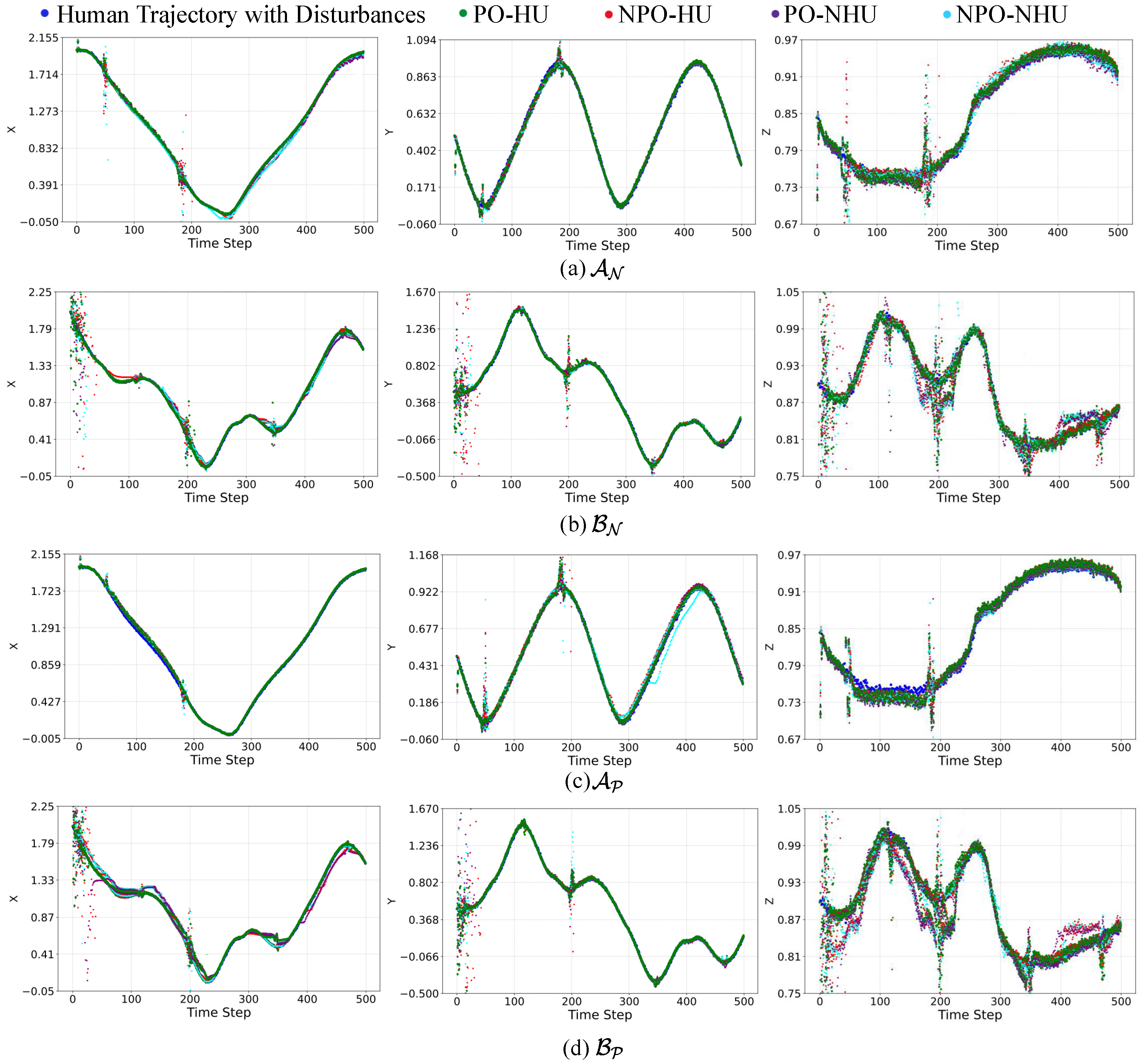
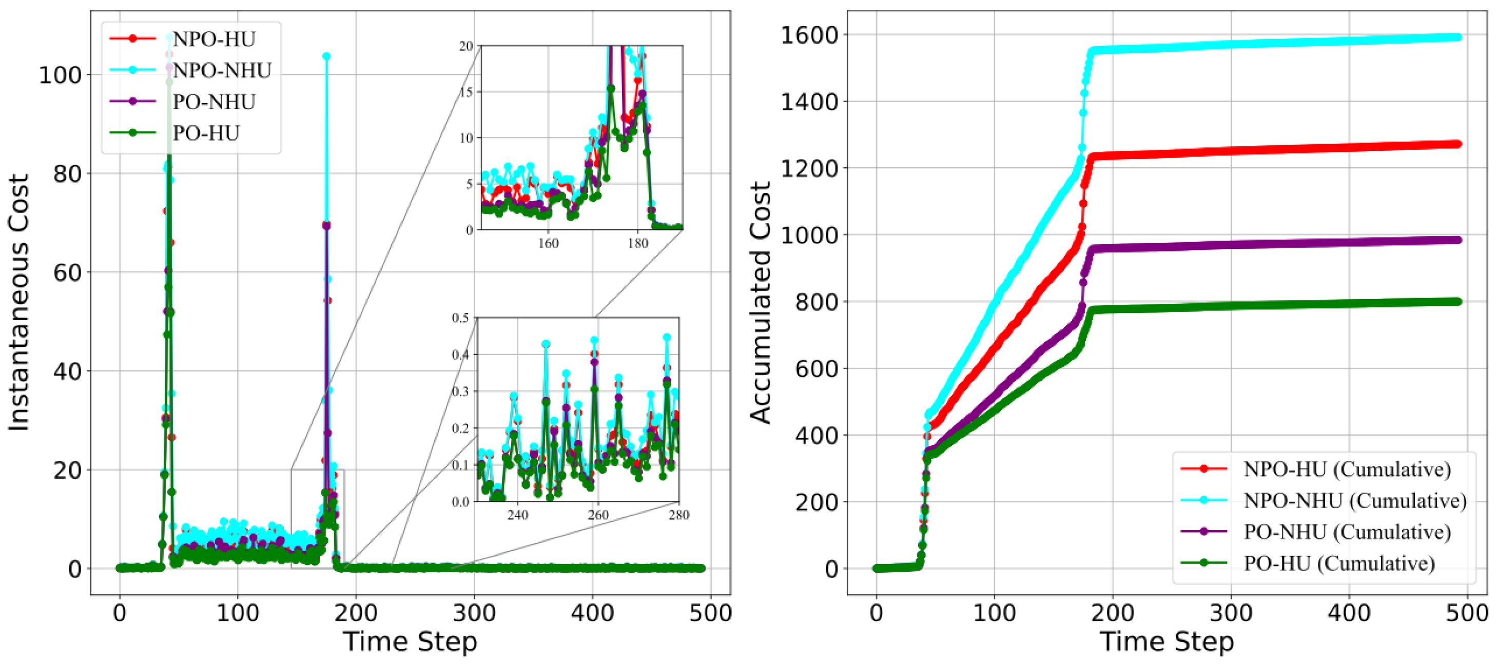
5.2. Evaluation of DARC Framework

We aim to validate the effectiveness of DARC under various levels of human disturbances and trajectories. We assumed that human uncertainties are mathematically equivalent to robot actuation disturbances, as discussed in Section 3.2. To model human uncertainties, we use $\varpi \left(k\right)\sim \mathcal{N}({\alpha }_{\varpi },{\Sigma }_{\varpi })$, where ${\alpha }_{\varpi }={[0.0035,0.0055,0.0027]}^{\top }$ (in meters) and ${\Sigma }_{\varpi }=\eta ·\mathrm{diag}(0.011,0.02,0.013)$ (in meters) and $\eta \in \{0.3,0.6\}$ represents the strength of the disturbances. This reflects the tendency for disturbances along the y-axis to be more pronounced than those in the x and z directions.

To evaluate the algorithm, we employ two representative trajectories, which are trajectory $\mathcal{A}$ and $\mathcal{B}$. Each of them is discretized with 500 waypoints and a time-step interval of $\mathsf{\Delta }t=0.1$ s. In one set of experiments, we assume that the future human poses are unknown to the robot. To address this, we incorporate an LSTM network for pose prediction (cf. Appendix A). The algorithm predicts the next six poses based on the ten previous poses. The experiments leveraging the LSTM-based prediction are denoted by ${\mathcal{A}}_{\mathcal{P}}$ and ${\mathcal{B}}_{\mathcal{P}}$. We consider a second set of experiments where we assume the future human pose to be fully known a priori, though still subject to disturbances. The corresponding experiments are denoted by ${\mathcal{A}}_{\mathcal{N}}$ and ${\mathcal{B}}_{\mathcal{N}}$.

We adopt an MPC strategy as described in Section 3.3 and in Algorithm 1, where the planning is repeated at every discrete time step. Within each planning horizon, we sample twenty candidate robot poses, i.e., $\left|\mathsf{\Theta }\right|=20$. To solve the optimization problem (5), we set $H=4$ for predictive experiments ${\mathcal{A}}_{\mathcal{P}}$ and ${\mathcal{B}}_{\mathcal{P}}$, and $H=8$ for the experiments ${\mathcal{A}}_{\mathcal{N}}$ and ${\mathcal{B}}_{\mathcal{N}}$. In the predictive cases, we forecast only six future steps. We chose $H=4(<6)$ to keep the planning horizon shorter than the prediction window. For ${\mathcal{A}}_{\mathcal{N}}$ and ${\mathcal{B}}_{\mathcal{N}}$, although the robot knows the full reference trajectory, setting a very long horizon would increase computational time and slow the solver. Thus, we select a moderate value $H=8$, which is double the predictive horizon. We examine two distinct settings for the tracking-error weight Q—i.e., $Q=1500·I_6$ and $Q=1100·I_6$. These configurations allow us to investigate the impact of reweighting the tracking error cost on the overall performance. A larger Q emphasizes pose tracking by rescaling the pose error to a magnitude comparable to the control inputs (unit-balancing). Moreover, it ensures the MPC actively suppresses the pose errors that might twist the object. We set $R=I_9$ to penalize all nine actuators evenly, which avoids over-regularizing of any specific control input. We set $\kappa =w_{\theta }=1$, which in our case, is sufficient to penalize changes in joint configurations.

Although the algorithm is designed to minimize an expected cost, we quantify the true cumulative cost over the full trajectory as follows:

$$\begin{array}{c}\hfill {\mathcal{C}}_{\mathrm{total}}=\sum _{t=1}^T\left[\mathit{e}{\left(t\right)}^{\top }Q\mathit{e}\left(t\right)+\mathit{u}{\left(t\right)}^{\top }R\mathit{u}\left(t\right)+\kappa {∥{\overline{\mathit{\theta }}}^{\ast }\left(t\right)-\mathit{\theta }\left(t\right)∥}_2^2\right],\end{array}$$

(20)

where the first term penalizes the end-effector tracking error, the second term penalizes the control effort, and the third term is related to pose optimization. $T=500$ denotes the total number of steps.

To evaluate the effectiveness of our proposed PO-HU algorithm with $\left|\mathsf{\Theta }\right|=20$, we compare it against five baseline methods: (i) PO-HU ($\left|\mathsf{\Theta }\right|=1$): single candidate pose optimization, which corresponds to using a traditional inverse kinematics approach that yields only one joint configuration; (ii) pPO-HU: periodic pose optimization every five time steps, which reduces computation load while still considering human uncertainty; (iii) NPO-HU: no pose optimization but considers human uncertainty while computing the control inputs; (iv) PO-NHU: perform pose optimization without considering the impact of human uncertainties; and (v) NPO-NHU: neither pose optimization nor human uncertainty is considered in the computation of the control inputs.

Table 3. Comparison of ${\mathcal{C}}_{\mathrm{total}}$ across different algorithms (mean ± standard deviation). ^†, ^‡, ^§ represent larger differences for NPO-HU, PO-NHU, and NPO-NHU, respectively, from PO-HU($\left|\mathsf{\Theta }\right|=20$).

Traj	Q	$\mathit{\eta }$	PO-HU ($|\mathbf{\Theta }|=20$)	PO-HU ($|\mathbf{\Theta }|=1$)	pPO-HU ($|\mathbf{\Theta }|=20$)	NPO-HU	PO-NHU	NPO-NHU
${\mathcal{A}}_{\mathcal{P}}$	$1500I_6$	0.3	879.02 ± 32.1	1012.59 ± 43.2	993.12 ± 38.7	2467.55 ± 158.4	1289.69 ± 52.1	8421.79 ± 402.1 §
		0.6	1008.45 ± 42.5	1289.51 ± 60.1	1217.44 ± 54.8	4664.03 ± 279.3 †	1855.11 ± 83.7 ‡	9107.12 ± 445.6 §
	$1100I_6$	0.3	911.56 ± 29.8	986.14 ± 38.5	957.71 ± 35.2	2395.09 ± 142.1	1051.24 ± 63.2	7916.18 ± 365.9 §
		0.6	994.99 ± 38.11	1079.52 ± 51.4	1042.36 ± 46.3	3674.88 ± 201.1 †	1102.45 ± 58.4	9363.44 ± 481.2 §
${\mathcal{A}}_{\mathcal{N}}$	$1500I_6$	0.3	799.66 ± 26.4	891.38 ± 36.5	851.45 ± 31.8	1271.54 ± 81.2	983.87 ± 56.2	1591.42 ± 102.4
		0.6	871.97 ± 36.1	968.91 ± 46.3	924.18 ± 42.6	1564.94 ± 104.8	1092.47 ± 64.9	3206.33 ± 189.7
	$1100I_6$	0.3	735.71 ± 30.1	809.48 ± 39.1	786.72 ± 35.6	1165.65 ± 75.4	869.09 ± 50.8	1778.19 ± 107.8
		0.6	861.07 ± 36.2	953.16 ± 45.8	902.42 ± 42.9	1334.66 ± 88.2	1013.35 ± 59.4	1819.98 ± 119.2
${\mathcal{B}}_{\mathcal{P}}$	$1500I_6$	0.3	852.84 ± 33.6	1091.48 ± 57.1	983.47 ± 43.4	1891.23 ± 127.4	1431.73 ± 71.3	5721.94 ± 314.5 §
		0.6	976.77 ± 43.1	1186.40 ± 61.7	1098.75 ± 54.3	2880.69 ± 162.2 †	1569.67 ± 77.8 ‡	6452.61 ± 338.4 §
	$1100I_6$	0.3	861.766 ± 30.2	1019.72 ± 49.1	971.33 ± 44.5	6407.73 ± 285.1 †	1260.28 ± 61.8	10531.81 ± 490.9 §
		0.6	1001.92 ± 43.4	1218.77 ± 59.1	1179.25 ± 53.7	7243.09 ± 327.8 †	1461.87 ± 70.5	11355.08 ± 517.6 §
${\mathcal{B}}_{\mathcal{N}}$	$1500I_6$	0.3	615.81 ± 26.1	701.63 ± 36.3	679.55 ± 33.7	1259.24 ± 92.1	764.59 ± 49.2	2558.78 ± 175.5
		0.6	828.87 ± 38.3	897.28 ± 52.6	866.41 ± 48.1	2483.88 ± 150.7	927.36 ± 62.1	3495.15 ± 198.8
	$1100I_6$	0.3	651.76 ± 32.1	762.99 ± 48.2	711.81 ± 39.5	2214.90 ± 12.3	969.85 ± 59.4	5278.04 ± 261.9 §
		0.6	778.93 ± 40.2	937.81 ± 59.4	894.11 ± 48.9	2758.48 ± 142.6 †	1172.75 ± 60.7	5661.65 ± 297.6 §

shows the mean with standard deviation of the total cost ${\mathcal{C}}_{\mathrm{total}}$ over 100 trials for each combination of trajectory type (${\mathcal{A}}_{\mathcal{P}}$, ${\mathcal{B}}_{\mathcal{P}}$, ${\mathcal{A}}_{\mathcal{N}}$, ${\mathcal{B}}_{\mathcal{N}}$), disturbance strength $\eta$, and weighting matrix Q. Here, we observe that whenever pose optimization is performed (i.e., PO-HU, PO-NHU, pPO-HU), it achieves a lower mean cost and often reduced standard deviation compared to methods lacking pose optimization (NPO-HU and NPO-NHU). Notably, NPO-NHU yields the highest mean cost with the largest variance as it neither performs pose optimization nor considers human uncertainties. This supports the importance of selecting a better pose for improved performance.

Within pose optimization methods, PO-HU outperforms PO-NHU. This reflects how explicitly accounting for human uncertainty yields advantages in all scenarios. While comparing PO-HU ($\left|\mathsf{\Theta }\right|=1$) and PO-HU ($\left|\mathsf{\Theta }\right|=20$), we observe that even a single-candidate version of pose optimization can achieve better results than not performing pose optimization at all, i.e., NPO-HU. However, when more candidate poses are considered ($\left|\mathsf{\Theta }\right|=20$), the algorithm better explores alternative joint configurations and achieves the lowest average total cost in all cases. Moreover, the pPO-HU shows that pose optimization at every five steps is still better than never performing pose optimization. Still, there exists a slight performance drop compared to optimizing at every time step.

In addition, NPO-HU shows better performance than NPO-NHU. This highlights that even without performing pose optimization, and only considering human uncertainty, it can still increase the overall performance. Here, we use specific markers to highlight significant differences with respect to PO-HU. We use “†” to mark large differences for NPO-HU, “‡” for PO-NHU, and “§” for NPO-NHU. The fewer highlighted markers in PO-NHU than in NPO-HU and NPO-NHU imply that pose optimization contributes more to cost reduction than the characterization of human uncertainty.

Overall, the robot achieves better performance in the cases where future human poses are known a priori to the robot (i.e., ${\mathcal{A}}_{\mathcal{N}}$ and ${\mathcal{B}}_{\mathcal{N}}$) compared to the cases where the robot uses LSTM to predict the human future poses (i.e., ${\mathcal{A}}_{\mathcal{P}}$ and ${\mathcal{B}}_{\mathcal{P}}$). This stems from having more accurate knowledge of human movements than predicting human poses.

Figure 5 visualizes the tracking performance along the x-, y-, and z-axes for trajectories ${\mathcal{A}}_{\mathcal{N}}$, ${\mathcal{B}}_{\mathcal{N}}$, ${\mathcal{A}}_{\mathcal{P}}$, and ${\mathcal{B}}_{\mathcal{P}}$, with the weighting matrix $Q=1500·I_6$ and $\eta =0.3$ for 10 representative trials. We observe that PO-HU tracks the human trajectory with disturbances more closely, whereas methods lacking pose optimization comparatively deviate more. Empirically, the performance of LSTM is good, as suggested by this figure. We observe that the human trajectories with disturbances in Figure 5c,d are almost similar to those in Figure 5a,b. We validated our trained LSTM model with trajectories ${\mathcal{A}}_{\mathcal{N}}$ and ${\mathcal{B}}_{\mathcal{N}}$. The validation accuracy of the model is $90.84\%$ with an MSE loss of 0.0512. If the human follows a smooth trajectory, it is expected that the model can predict the future movements with high accuracy. Theoretically, the accuracy of the LSTM-based model is not guaranteed. If the human takes sharp turns, then the trajectory prediction accuracy will be lower. Consequently, the control cost obtained from the MPC can be inaccurate, which further impacts the pose selection. However, when the control input is implemented, the tracking accuracy will not be significantly impacted, as we have a closed-loop control. Specifically, while the MPC can plan for six future time steps, the execution applies to only one step.

Figure 6 depicts the instantaneous (left) and accumulated cost (right) for trajectory ${\mathcal{A}}_{\mathcal{N}}$ with $Q=1500·I_6$, $R=I_9$, and $\eta =0.3$. We observe that, at each time step, the cost associated with PO-HU remains the lowest, while NPO-NHU consistently shows the highest cost. This reflects that incorporating pose optimization performs better than ignoring it, both in terms of instantaneous and accumulated cost.

Table 4. Average tracking error with standard deviation of trajectories for different planning horizons with PO-HU.

Trajectory	H = 1	H = 4	H = 6	H = 8
${\mathcal{A}}_{\mathcal{P}}$	0.049 ± 0.027	0.072 ± 0.027	0.091 ± 0.031	0.104 ± 0.039
${\mathcal{A}}_{\mathcal{N}}$	0.034 ± 0.019	0.056 ± 0.034	0.072 ± 0.038	0.082 ± 0.043
${\mathcal{B}}_{\mathcal{P}}$	0.041 ± 0.024	0.062 ± 0.039	0.077 ± 0.045	0.085 ± 0.049
${\mathcal{B}}_{\mathcal{N}}$	0.031 ± 0.017	0.057 ± 0.031	0.065 ± 0.035	0.075 ± 0.038

Note: Bold entries represent the lowest average tracking error for each trajectory across planning horizons.

represents the comparison of average tracking error (mean ± standard deviation) across different planning horizons for the proposed PO-HU method. This tracking error is averaged over 100 trials. We observe that a longer planning horizon may increase tracking error if we execute the entire control input sequence. For example, when $H=8$, executing all eight control inputs may incur a higher tracking error. In our method, although we generate the eight control inputs for the future eight time steps, we only execute the control input for the first time step, and then re-plan again for the next planning horizon. This strategy yields a lower tracking error, as shown in the case of a planning horizon of $H=1$.

Table 5. Average execution time with standard deviation in evaluating each candidate for different planning horizons with $\left|\mathsf{\Theta }\right|=20$ (in seconds).

Planning Horizon	PO-HU	NPO-HU	PO-NHU
4	0.013286 ± 0.00116	0.010474 ± 0.00094	0.013164 ± 0.00102
8	0.013633 ± 0.00121	0.011300 ± 0.00109	0.013295 ± 0.00107
12	0.013866 ± 0.00119	0.012736 ± 0.00113	0.013668 ± 0.00115
16	0.014126 ± 0.00124	0.012807 ± 0.00119	0.014003 ± 0.00119
20	0.014951 ± 0.00128	0.013287 ± 0.00116	0.014205 ± 0.00124
24	0.015287 ± 0.00131	0.013888 ± 0.00125	0.014257 ± 0.00129

presents the average execution time with standard deviation in evaluating each candidate for different planning horizons. The time is averaged over 500 trials. In our approach, we can parallelize steps 4–9 of Algorithm 1. As a result, the computation times for methods with and without pose optimization differ slightly. This benefits from the multiple computing threads of the AMD 5975WX on our test computer. The majority of the computation time is spent on the one-time calculation of the Jacobian matrix. The minor increase is due to the increasing number of planning horizons and thus more iterations when solving the DARE (cf. Equation (8)).

5.3. Hardware Demonstration

Besides Gazebo simulations, we implemented our proposed algorithm in real hardware as a demo. A video of the hardware demo is available at https://www.youtube.com/watch?v=QyR2NcSXhvY (accessed on 16 June 2025). For this hardware demo, we used an AprilTag marker on a board and placed a cup on top. We allowed the robot to capture the marker’s pose with its built-in camera for end-effector tracking. We positioned the cup so that the marker remained visible to the camera. The captured pose was first obtained in the camera frame, and then it was transformed to the robot’s base frame using the tf package. The human leads the robot by pulling the board along the x, y, and z axes. The robot predicts six future poses using LSTM, and uses a planning horizon of $H=3$. It then plans three steps with MPC but executes only the first control input before re-planning to adapt to the human. We used $Q=1100·I_6$, $R=I_9$, and $\kappa =w_{\theta }=1$ in the demonstration. As discussed in Section 3, each control input consists of the linear and angular velocity of the base and seven joint angle velocities. The executions of these control inputs are driven by an ROS publisher and then sent to the corresponding ROS topic on Fetch. From the demonstration video, we observe that tracking is slower. This is primarily due to the physical execution time required for the robot to move its base and arm. The computation time does not significantly impact the slowness of the demonstration, as the generation of the candidate set is achieved by the pre-trained CVAE model, and the evaluation of each candidate was fully parallelized throughout the demonstration.

6. Conclusions and Future Works

We proposed and validated the Disturbance-Aware Redundant Control (DARC) framework, which integrates disturbance-aware MPC with a proactive pose optimization strategy for efficient human–robot co-transportation. The developed two-step iterative approach effectively addresses the inherent uncertainties of human behavior and internal robot disturbances by proactively generating and selecting robot joint configurations. To facilitate this process, we utilized a Conditional Variational Autoencoder (CVAE) to generate candidate sets of joint configurations for pose optimization, while a Long Short-Term Memory (LSTM) network was employed to predict future human poses. Theoretical derivations and simulated experiments with a Fetch mobile manipulator demonstrate the enhanced performance of our proposed framework compared to control methodologies that lack disturbance characterization or pose optimization. Future work will aim to refine the modeling of human behavior and decision-making processes and extend the proposed DARC framework to complex scenarios involving multi-robot multi-human collaborative tasks.

References

1. Prewett, M.S.; Johnson, R.C.; Saboe, K.N.; Elliott, L.R.; Coovert, M.D. Managing workload in human–robot interaction: A review of empirical studies. Comput. Hum. Behav. 2010, 26, 840–856. [Google Scholar] [CrossRef]
2. Liu, L.; Schoen, A.J.; Henrichs, C.; Li, J.; Mutlu, B.; Zhang, Y.; Radwin, R.G. Human robot collaboration for enhancing work activities. Hum. Factors 2024, 66, 158–179. [Google Scholar] [CrossRef] [PubMed]
3. Bischoff, R.; Kurth, J.; Schreiber, G.; Koeppe, R.; Albu-Schäffer, A.; Beyer, A.; Eiberger, O.; Haddadin, S.; Stemmer, A.; Grunwald, G.; et al. The KUKA-DLR Lightweight Robot arm—A new reference platform for robotics research and manufacturing. In Proceedings of the ISR 2010 (41st International Symposium on Robotics) and ROBOTIK 2010 (6th German Conference on Robotics), Munich, Germany, 7–9 June 2010; VDE: Berlin, Germany; pp. 1–8. [Google Scholar]
4. Pedrocchi, N.; Vicentini, F.; Matteo, M.; Tosatti, L.M. Safe human-robot cooperation in an industrial environment. Int. J. Adv. Robot. Syst. 2013, 10, 27. [Google Scholar] [CrossRef]
5. Broekens, J.; Heerink, M.; Rosendal, H. Assistive social robots in elderly care: A review. Gerontechnology 2009, 8, 94–103. [Google Scholar] [CrossRef]
6. Cai, S.; Ram, A.; Gou, Z.; Shaikh, M.A.W.; Chen, Y.A.; Wan, Y.; Hara, K.; Zhao, S.; Hsu, D. Navigating real-world challenges: A quadruped robot guiding system for visually impaired people in diverse environments. In Proceedings of the 2024 CHI Conference on Human Factors in Computing Systems, Honolulu, HI, USA, 11–16 May 2024; pp. 1–18. [Google Scholar]
7. Ajoudani, A.; Zanchettin, A.M.; Ivaldi, S.; Albu-Schäffer, A.; Kosuge, K.; Khatib, O. Progress and prospects of the human–robot collaboration. Auton. Robot. 2018, 42, 957–975. [Google Scholar] [CrossRef]
8. Sharkawy, A.N.; Koustoumpardis, P.N. Human–robot interaction: A review and analysis on variable admittance control, safety, and perspectives. Machines 2022, 10, 591. [Google Scholar] [CrossRef]
9. Hayes, B.; Scassellati, B. Challenges in shared-environment human-robot collaboration. Learning 2013, 8. [Google Scholar]
10. Brosque, C.; Galbally, E.; Khatib, O.; Fischer, M. Human-robot collaboration in construction: Opportunities and challenges. In Proceedings of the 2020 IEEE International Congress on Human-Computer Interaction, Optimization and Robotic Applications (HORA), Ankara, Turkey, 26–28 June 2020; pp. 1–8. [Google Scholar]
11. Cursi, F.; Modugno, V.; Lanari, L.; Oriolo, G.; Kormushev, P. Bayesian neural network modeling and hierarchical MPC for a tendon-driven surgical robot with uncertainty minimization. IEEE Robot. Autom. Lett. 2021, 6, 2642–2649. [Google Scholar] [CrossRef]
12. Mahmud, A.J.; Li, W.; Wang, X. Mutual Adaptation in Human-Robot Co-Transportation with Human Preference Uncertainty. arXiv 2025, arXiv:2503.08895. [Google Scholar]
13. Haninger, K.; Hegeler, C.; Peternel, L. Model predictive control with gaussian processes for flexible multi-modal physical human robot interaction. In Proceedings of the 2022 IEEE International Conference on Robotics and Automation (ICRA), Philadelphia, PA, USA, 23–27 May 2022; pp. 6948–6955. [Google Scholar]
14. Donelan, P. Singularities of robot manipulators. In Singularity Theory: Dedicated to Jean-Paul Brasselet on His 60th Birthday; World Scientific: Singapore, 2007; pp. 189–217. [Google Scholar]
15. Chiaverini, S. Singularity-robust task-priority redundancy resolution for real-time kinematic control of robot manipulators. IEEE Trans. Robot. Autom. 1997, 13, 398–410. [Google Scholar] [CrossRef]
16. Chiacchio, P.; Chiaverini, S.; Sciavicco, L.; Siciliano, B. Closed-loop inverse kinematics schemes for constrained redundant manipulators with task space augmentation and task priority strategy. Int. J. Robot. Res. 1991, 10, 410–425. [Google Scholar] [CrossRef]
17. Wittmann, J.; Kist, A.; Rixen, D.J. Real-Time Predictive Kinematics Control of Redundancy: A Benchmark of Optimal Control Approaches. In Proceedings of the 2022 IEEE/RSJ International Conference on Intelligent Robots and Systems (IROS), Kyoto, Japan, 23–27 October 2022; pp. 11759–11766. [Google Scholar]
18. Faroni, M.; Beschi, M.; Tosatti, L.M.; Visioli, A. A predictive approach to redundancy resolution for robot manipulators. IFAC-Pap. Online 2017, 50, 8975–8980. [Google Scholar] [CrossRef]
19. Erhart, S.; Sieber, D.; Hirche, S. An impedance-based control architecture for multi-robot cooperative dual-arm mobile manipulation. In Proceedings of the 2013 IEEE/RSJ International Conference on Intelligent Robots and Systems, Tokyo, Japan, 3–7 November 2013; pp. 315–322. [Google Scholar]
20. Mahmud, A.J.; Raj, A.H.; Nguyen, D.M.; Xiao, X.; Wang, X. Human-Robot Co-Transportation with Human Uncertainty-Aware MPC and Pose Optimization. arXiv 2024, arXiv:2404.00514. [Google Scholar]
21. Aaltonen, I.; Salmi, T.; Marstio, I. Refining levels of collaboration to support the design and evaluation of human-robot interaction in the manufacturing industry. Procedia CIRP 2018, 72, 93–98. [Google Scholar] [CrossRef]
22. Magrini, E.; Ferraguti, F.; Ronga, A.J.; Pini, F.; De Luca, A.; Leali, F. Human-robot coexistence and interaction in open industrial cells. Robot. Comput.-Integr. Manuf. 2020, 61, 101846. [Google Scholar] [CrossRef]
23. Roveda, L.; Maskani, J.; Franceschi, P.; Abdi, A.; Braghin, F.; Molinari Tosatti, L.; Pedrocchi, N. Model-based reinforcement learning variable impedance control for human-robot collaboration. J. Intell. Robot. Syst. 2020, 100, 417–433. [Google Scholar] [CrossRef]
24. Peternel, L.; Tsagarakis, N.; Caldwell, D.; Ajoudani, A. Robot adaptation to human physical fatigue in human–robot co-manipulation. Auton. Robot. 2018, 42, 1011–1021. [Google Scholar] [CrossRef]
25. Mujica, M.; Crespo, M.; Benoussaad, M.; Junco, S.; Fourquet, J.Y. Robust variable admittance control for human–robot co-manipulation of objects with unknown load. Robot. Comput.-Integr. Manuf. 2023, 79, 102408. [Google Scholar] [CrossRef]
26. Zhang, Y.; Pezzato, C.; Trevisan, E.; Salmi, C.; Corbato, C.H.; Alonso-Mora, J. Multi-Modal MPPI and Active Inference for Reactive Task and Motion Planning. IEEE Robot. Autom. Lett. 2024, 9, 7461–7468. [Google Scholar] [CrossRef]
27. Bhardwaj, M.; Sundaralingam, B.; Mousavian, A.; Ratliff, N.D.; Fox, D.; Ramos, F.; Boots, B. Storm: An integrated framework for fast joint-space model-predictive control for reactive manipulation. In Proceedings of the Conference on Robot Learning, Auckland, New Zealand, 14–18 December 2022; pp. 750–759. [Google Scholar]
28. De Schepper, D.; Schouterden, G.; Kellens, K.; Demeester, E. Human-robot mobile co-manipulation of flexible objects by fusing wrench and skeleton tracking data. Int. J. Comput. Integr. Manuf. 2023, 36, 30–50. [Google Scholar] [CrossRef]
29. Sirintuna, D.; Giammarino, A.; Ajoudani, A. An Object Deformation-Agnostic Framework for Human–Robot Collaborative Transportation. IEEE Trans. Autom. Sci. Eng. 2023, 21, 1986–1999. [Google Scholar] [CrossRef]
30. Sirintuna, D.; Ozdamar, I.; Gandarias, J.M.; Ajoudani, A. Enhancing Human-Robot Collaboration Transportation through Obstacle-Aware Vibrotactile Feedback. arXiv 2023, arXiv:2302.02881. [Google Scholar]
31. Bussy, A.; Gergondet, P.; Kheddar, A.; Keith, F.; Crosnier, A. Proactive behavior of a humanoid robot in a haptic transportation task with a human partner. In Proceedings of the 2012 IEEE RO-MAN: The 21st IEEE International Symposium on Robot and Human Interactive Communication, Paris, France, 9–13 September 2012; pp. 962–967. [Google Scholar]
32. Agravante, D.J.; Cherubini, A.; Sherikov, A.; Wieber, P.B.; Kheddar, A. Human-humanoid collaborative carrying. IEEE Trans. Robot. 2019, 35, 833–846. [Google Scholar] [CrossRef]
33. Berger, E.; Vogt, D.; Haji-Ghassemi, N.; Jung, B.; Amor, H.B. Inferring guidance information in cooperative human-robot tasks. In Proceedings of the 2013 13th IEEE-RAS International Conference on Humanoid Robots (Humanoids), Atlanta, GA, USA, 15–17 October 2013; pp. 124–129. [Google Scholar]
34. Zanon, M.; Gros, S. Safe reinforcement learning using robust MPC. IEEE Trans. Autom. Control 2020, 66, 3638–3652. [Google Scholar] [CrossRef]
35. Saltık, M.B.; Özkan, L.; Ludlage, J.H.; Weiland, S.; Van den Hof, P.M. An outlook on robust model predictive control algorithms: Reflections on performance and computational aspects. J. Process Control 2018, 61, 77–102. [Google Scholar] [CrossRef]
36. Mohammadpour, J.; Scherer, C.W. Control of Linear Parameter Varying Systems with Applications; Springer Science & Business Media: Berlin, Germany, 2012. [Google Scholar]
37. Patel, S.; Sobh, T. Manipulator performance measures-a comprehensive literature survey. J. Intell. Robot. Syst. 2015, 77, 547–570. [Google Scholar] [CrossRef]
38. Yoshikawa, T. Manipulability of robotic mechanisms. Int. J. Robot. Res. 1985, 4, 3–9. [Google Scholar] [CrossRef]
39. Cheong, H.; Ebrahimi, M.; Duggan, T. Optimal design of continuum robots with reachability constraints. IEEE Robot. Autom. Lett. 2021, 6, 3902–3909. [Google Scholar] [CrossRef]
40. Mohammed, A.; Schmidt, B.; Wang, L.; Gao, L. Minimizing energy consumption for robot arm movement. Procedia Cirp 2014, 25, 400–405. [Google Scholar] [CrossRef]
41. Zhang, M.M.; Atanasov, N.; Daniilidis, K. Active end-effector pose selection for tactile object recognition through monte carlo tree search. In Proceedings of the 2017 IEEE/RSJ International Conference on Intelligent Robots and Systems (IROS), Vancouver, BC, Canada, 24–28 September 2017; pp. 3258–3265. [Google Scholar]
42. Wang, J.; Zhang, T.; Wang, Y.; Luo, D. Optimizing Robot Arm Reaching Ability with Different Joints Functionality. In Proceedings of the 2023 32nd IEEE International Conference on Robot and Human Interactive Communication (RO-MAN), Busan, Republic of Korea, 28–31 August 2023; pp. 1778–1785. [Google Scholar]
43. Schneider, U.; Posada, J.R.D.; Verl, A. Automatic pose optimization for robotic processes. In Proceedings of the 2015 IEEE International Conference on Robotics and Automation (ICRA), Seattle, WA, USA, 26–30 May 2015; pp. 2054–2059. [Google Scholar]
44. George Thuruthel, T.; Ansari, Y.; Falotico, E.; Laschi, C. Control strategies for soft robotic manipulators: A survey. Soft Robot. 2018, 5, 149–163. [Google Scholar] [CrossRef]
45. Kumar, V.; Hoeller, D.; Sundaralingam, B.; Tremblay, J.; Birchfield, S. Joint space control via deep reinforcement learning. In Proceedings of the 2021 IEEE/RSJ International Conference on Intelligent Robots and Systems (IROS), Prague, Czech Republic, 27 September–1 October 2021; pp. 3619–3626. [Google Scholar]
46. Hua, X.; Wang, G.; Xu, J.; Chen, K. Reinforcement learning-based collision-free path planner for redundant robot in narrow duct. J. Intell. Manuf. 2021, 32, 471–482. [Google Scholar] [CrossRef]
47. Shen, Y.; Jia, Q.; Huang, Z.; Wang, R.; Fei, J.; Chen, G. Reinforcement learning-based reactive obstacle avoidance method for redundant manipulators. Entropy 2022, 24, 279. [Google Scholar] [CrossRef] [PubMed]
48. Soleimani Amiri, M.; Ramli, R. Intelligent trajectory tracking behavior of a multi-joint robotic arm via genetic–swarm optimization for the inverse kinematic solution. Sensors 2021, 21, 3171. [Google Scholar] [CrossRef] [PubMed]
49. Parque, V.; Miyashita, T. Smooth curve fitting of mobile robot trajectories using differential evolution. IEEE Access 2020, 8, 82855–82866. [Google Scholar] [CrossRef]
50. Sun, L.; Zhan, W.; Hu, Y.; Tomizuka, M. Interpretable modelling of driving behaviors in interactive driving scenarios based on cumulative prospect theory. In Proceedings of the 2019 IEEE Intelligent Transportation Systems Conference (ITSC), Auckland, New Zealand, 27–30 October 2019; pp. 4329–4335. [Google Scholar]
51. Zhang, J.; Liu, H.; Chang, Q.; Wang, L.; Gao, R.X. Recurrent neural network for motion trajectory prediction in human-robot collaborative assembly. CIRP Ann. 2020, 69, 9–12. [Google Scholar] [CrossRef]
52. Kratzer, P.; Toussaint, M.; Mainprice, J. Prediction of human full-body movements with motion optimization and recurrent neural networks. In Proceedings of the 2020 IEEE International Conference on Robotics and Automation (ICRA), Paris, France, 31 May–31 August 2020; pp. 1792–1798. [Google Scholar]
53. Alahi, A.; Goel, K.; Ramanathan, V.; Robicquet, A.; Fei-Fei, L.; Savarese, S. Social lstm: Human trajectory prediction in crowded spaces. In Proceedings of the IEEE Conference on Computer Vision and Pattern Recognition, Las Vegas, NV, USA, 27–30 June 2016; pp. 961–971. [Google Scholar]
54. Manh, H.; Alaghband, G. Scene-lstm: A model for human trajectory prediction. arXiv 2018, arXiv:1808.04018. [Google Scholar]
55. Rossi, L.; Paolanti, M.; Pierdicca, R.; Frontoni, E. Human trajectory prediction and generation using LSTM models and GANs. Pattern Recognit. 2021, 120, 108136. [Google Scholar] [CrossRef]
56. Fetch Robotics. Fetch & Freight Research Edition Documentation. Available online: https://github.com/fetchrobotics/docs (accessed on 16 June 2025).
57. Campa, R.; De La Torre, H. Pose control of robot manipulators using different orientation representations: A comparative review. In Proceedings of the 2009 IEEE American Control Conference, St. Louis, MO, USA, 10–12 June 2009; pp. 2855–2860. [Google Scholar]
58. Zheng, H.; Negenborn, R.R.; Lodewijks, G. Trajectory tracking of autonomous vessels using model predictive control. IFAC Proc. Vol. 2014, 47, 8812–8818. [Google Scholar] [CrossRef]
59. Shi, Q.; Zhao, J.; El Kamel, A.; Lopez-Juarez, I. MPC based vehicular trajectory planning in structured environment. IEEE Access 2021, 9, 21998–22013. [Google Scholar] [CrossRef]
60. Ho, C.K.; Chan, L.W.; King, C.T.; Yen, T.Y. A deep learning approach to navigating the joint solution space of redundant inverse kinematics and its applications to numerical IK computations. IEEE Access 2023, 11, 2274–2290. [Google Scholar] [CrossRef]
61. Dozat, T. Incorporating Nesterov Momentum into Adam. In Proceedings of the International Conference on Learning Representations (ICLR), San Juan, Puerto Rico, 2–4 May 2016; pp. 1–4. [Google Scholar]
Figure 1. Human–robot co-transportation through disturbance-aware MPC and pose optimization (redundancy resolution for the same end-effector position).
Electronics 14 02480 g001
Figure 2. (a,b) show the Fetch robot’s mobile base and arm configuration. (a) Fetch robot’s base in the inertial frame. A shifted frame Ξ centered at the robot’s current position. (b) Denavit–Hartenberg (DH) representation with 8-DOF (manipulator’s joint angles and base’s heading angle) joint configurations in Ξ frame.
Electronics 14 02480 g002
Figure 3. Block diagram model of CVAE for pose optimization.
Electronics 14 02480 g003
Figure 4. Visualization of CVAE model training metrics and outputs: (af) show various training and evaluation plots including loss, accuracy, MSE, predicted vs. desired outputs, and joint variations. (a) Training and validation loss of the CVAE model. (b) Training and validation accuracy of the CVAE model. (c) MSE between predicted and desired end-effector pose. (d) Predicted vs. desired end-effector position. (e) Predicted vs. desired end-effector orientation. (f) Variation in joint angles from the given joint angle.
Electronics 14 02480 g004
Figure 5. Tracking across trajectories (a) A N , (b) B N , (c) A P , and (d) B P on the x-, y-, and z-axes, where Q = 1500 · I 6 , R = I 9 , and η = 0.3 for 10 representative trials.
Electronics 14 02480 g005
Figure 6. Instantaneous and accumulated cost for trajectory A N with Q = 1500 · I 6 , R = I 9 , and η = 0.3 .
Electronics 14 02480 g006