BO–FTT: A Deep Learning Model Based on Parameter Tuning for Early Disease Prediction from a Case of Anemia in CKD

Abstract

Renal anemia (RA) is a common complication of chronic kidney disease (CKD). Patients with prolonged RA may present with nonspecific systemic manifestations, including cold intolerance, fatigue, drowsiness, anorexia, muscle weakness, reduced physical activity, impaired memory and cognitive function, and difficulty concentrating. Although previous studies have identified risk factors for anemia development in CKD, challenges remain in early diagnosis and therapeutic intervention. Therefore, we analyzed a dataset of CKD patients with RA from the MIMIC database and used machine learning models to predict whether RA will occur in CKD patients. In addition, an optimized model was designed, and is explained in the article, that tunes the hyperparameters of FT-Transformer (FTT) with the Bayesian optimization (BO) algorithm. The proposed BO–FTT model achieved an accuracy of 91.81%, outperforming the untuned FTT as well as TabNet, Multilayer Perceptron (MLP), and Kolmogorov–Arnold Networks (KAN) that were optimized by the BO algorithm.

1. Introduction

Chronic kidney disease (CKD) is a prevalent clinical renal disease, the main cause of which is chronic and persistent impairment of renal function [1]. Nowadays, the global incidence of CKD is increasing annually. Due to its long latency period, difficult detection, and poor prognosis, CKD has been recognized as a major public health challenge globally [2]. According to the National Health and Nutrition Examination Survey (NHANES) study, the total prevalence of CKD is already at 11.7% and is expected to rise to 16.7% by 2030 [3,4]. Such a high prevalence has a serious impact on individual health and presents a significant challenge to socioeconomic and public health systems.

Clinically, CKD patients frequently develop renal anemia (RA), secondary hyperparathyroidism (SHPT), and other comorbidities [5]. Among these complications, RA is one of the most common manifestations of CKD. It is characterized by anemia resulting from reduced renal erythropoietin (EPO) production and the accumulation of plasma toxins that impair erythropoiesis and shorten red blood cell lifespan as renal function deteriorates due to underlying kidney diseases [6,7]. RA has been demonstrated to exacerbate renal disease progression, and patients with anemia due to CKD have a higher mortality rate than CKD patients without RA. If RA patients are not diagnosed and treated promptly, other diseases are likely to be induced, which can cause death in severe situations [8,9]. As a result, when patients are diagnosed with CKD, early assessment of RA risk is critical to initiate timely interventions, thereby improving clinical outcomes and quality of life.

However, the complexity of factors contributing to the increased risk of anemia in CKD and the lack of consensus on specific diagnostic markers have led to difficulty in early prediction and timely therapeutic decisions [10]. Therefore, there is an urgent need for efficient and accurate methods to support doctors in making a diagnosis and designing clinical studies on CKD.

Artificial intelligence and big data have advanced rapidly since the beginning of the 21st century, and the application of machine learning (ML) algorithms in disease prediction has received increasing attention. ML is a data-driven approach that can improve performance by tuning hyperparameters and optimizing algorithms. It is widely used in disease diagnosis and prognosis [11]. Therefore, the goal of this paper was to design an early prediction model using ML algorithms, which would be applied to estimate the probability of anemia in CKD patients and identify key biomarkers associated with renal anemia pathogenesis.

The contributions of this work are as follows:

• Medical data of CKD and RA patients were extracted from the MIMIC database and preprocessed. To ensure analytical reliability, we implemented three distinct feature selection methods and addressed dataset imbalance through targeted techniques.
• We designed a model that tuned the hyperparameters of FT-Transformer using the Bayesian optimization algorithm. By continuously optimizing the parameters and improving the classifier’s performance, we successfully achieved accurate predictions about the likelihood of CKD patients developing RA.
• A comprehensive evaluation and interpretability analysis were conducted on the trained model, through which key risk factors predictive of clinical outcomes were identified. By integrating these findings with the existing medical literature, we further validated the identified risk factors, strengthening their clinical relevance and implications.

Figure 1 depicts the technology roadmap for the remaining parts of this study. The pathogenesis and diagnostic advances of RA and the application of ML in the early prediction of renal diseases are presented in “Section 2”. “Section 3” introduces the dataset and the methodology in the experiment, including data preprocessing, feature selection, and the construction of deep learning models based on hyperparameter optimization. In “Section 4”, the performance of the model designed in the paper is evaluated using evaluation metrics, and a series of comparative experiments are conducted. Lastly, the experimental conclusions are summarized, and future research directions are presented in “Section 5”.

2. Related Work

RA is a common complication of CKD, which is caused mostly by reduced renal EPO production and iron deficiency. However, the diagnosis of anemia in individuals with CKD is challenging. For example, the gold-standard indicator for iron deficiency anemia, such as bone marrow iron storage, is invasive, or some individuals may not respond well to erythropoiesis despite iron supplementation [12]. As a result, we will start by discussing the markers that have potential in the diagnosis of RA.

Agoro et al. [13] discovered that inhibiting FGF-23 signaling can significantly slow down the apoptosis of erythroid cells, promote the mRNA expression of EPO, and diminish the expression of HIF-1α and HIF-2α, thereby creating a hypoxic environment conducive to stimulate erythropoiesis. The experiment further confirmed that FGF 23 inhibits the expression of ferredoxin and inflammatory factors, leading to increased serum iron and reduced inflammation. Tirmenstajn-Jankovic et al. [14] investigated patients with CKD stages 3–5 and found that anemia and renal dysfunction were independently associated with NT-proBNP (BNP) levels. Anemia can cause an increase in heart rate to obstruct oxygen delivery, potentially leading to ventricular remodeling. Furthermore, anemia can impair myocardial oxygen supply and increase cardiac burden by stimulating the sympathetic nervous system and the renin–angiotensin–aldosterone system, which further influences BNP levels. It was observed that creatinine and BNP levels were significantly higher in anemic patients with advanced CKD compared to non-anemic patients. Din et al. [15] examined laboratory tests in hemodialysis patients, which included serum calcium, phosphorus, 25(OH) vitamin D, intact parathyroid hormone (iPTH) levels, hemoglobin level, ferritin level, serum iron, total iron binding capacity, and transferrin saturation. Significant correlations were found between vitamin D levels, iPTH levels, calcium, and hemoglobin levels according to the experiment results. Kamei et al. [16] studied hemodialysis patients and utilized Passing–Bablok regression analysis to evaluate the methods in this experiment. The results revealed a significant correlation between the hepcidin-25 levels assessed by latex immunoassay (LIA) and liquid chromatography–tandem mass spectrometry (LC-MS/MS), with nearly equivalent measurements. As a result, a high level of hepcidin can support predicting the severity of anemia in CKD patients, with better performance in advanced CKD patients with severe anemia. Akchurin et al. [17] investigated the serum parameters of pediatric CKD patients and found that, after adjusting for the glomerular filtration rate (GFR), only IL-6 was significantly inversely associated with hemoglobin levels. The relationship between IL-6 and hemoglobin in children with CKD remained strong even after controlling for the CKD stage and iron-modulating hormones. This suggested that IL-6 plays a crucial role in the inflammatory process related to RA, and it may exacerbate anemia not only by affecting iron metabolism but also by promoting renal fibrosis and interfering with the normal function of EPO. These findings provided a theoretical foundation for the development of new diagnostic and predictive approaches for anemia in CKD.

ML is a branch of artificial intelligence that focuses on the development of algorithms and statistical models; it can be subdivided into supervised learning and unsupervised learning, and supervised learning algorithms include K-nearest neighbor (KNN), naive Bayes (NB), support vector machine (SVM), logistic regression (LR), neural network (NN), decision tree (DT), and ensemble models of DT such as random forest (RF), extreme gradient boosting (XGBoost), and light gradient boosting machine (LightGBM) [18]. Among these ML algorithms, neural networks (NNs) are computational models inspired by biological nervous systems, with common examples including Multilayer Perceptron (MLP). NN can further develop into deep learning, which has a more complex structure and can process more information. Common deep learning models include convolutional neural networks (CNN) and recurrent neural networks (RNN). Some researchers have also presented new deep learning models subsequently. For instance, Vaswani et al. [19] presented the Transformer in 2017, illustrating the ongoing advancement and improvement of ML algorithms in handling tasks with intricate information. In recent years, supervised learning algorithms have been widely used in the prediction of kidney diseases. Therefore, the following chapters will introduce the application of ML in kidney diseases, using acute kidney injury (AKI), CKD, and diabetic nephropathy (DN) as examples.

AKI is one of the most common kidney diseases. Tomašev et al. [20] designed a prediction model for AKI based on a large longitudinal electronic health record using deep learning algorithms. The model could predict 55.8% of AKI events in hospitalized patients. In addition, the model was able to predict future trends in clinical blood tests, which may provide a time window to identify patients at risk and provide early treatment. To study the early prediction of Sepsis-Associated AKI, Yue et al. [21] extracted medical data of sepsis patients from the MIMIC database and selected features by utilizing the Boruta algorithm with ten-fold cross-validation. They used multiple ML models, including LR, KNN, SVM, DT, RF, ANN, and XGBoost, and compared them with the traditional SOFA and SAPS II scoring models. The results showed that the XGBoost achieved a maximum AUC value of 0.7787 with better performance. She et al. [22] also predicted the risk of AKI in patients with intracerebral hemorrhage (ICH) based on the MIMIC database. In the training set, six ML algorithms, including XGBoost, LR, LightGBM, RF, AdaBoost, and MLP, were trained using a five-fold cross-validation method. The results showed that, among the six ML algorithms, RF achieved the maximum AUC value of 0.698 on the validation set. The most important features ranked based on the RF algorithm were platelets, serum creatinine, vancomycin, hemoglobin, and hematocrit. Qu et al. [23] analyzed the data of patients with acute pancreatitis for the occurrence of AKI by several ML methods. Their study retrieved information such as demographic characteristics and laboratory data, and the dataset was input into the SVM, RF, CART, and XGBoost models. In the experiment, XGBoost obtained the highest AUC value of 0.91. Zhang et al. [24] similarly analyzed patients with acute pancreatitis and constructed an AutoML model to compare with the traditional LR model. The results demonstrated that the deep learning model excelled in predicting AKI in patients with acute pancreatitis, achieving an AUC of 0.83 on the validation set. Meanwhile, the article identified creatinine, urea, International Normalized Ratio (INR), etiology, smoking status, alanine aminotransferase (ALT), hypertension, prothrombin time (PT), lactate dehydrogenase (LDH), and diabetes mellitus as important factors affecting the prediction of AKI in patients with acute pancreatitis through interpretability analysis.

CKD is a renal disease characterized by chronic structural and renal dysfunction due to a variety of causes. Chang et al. [25] used the Cox proportional hazards (PH) model to predict the risk of progression to dialysis in patients with CKD by collecting demographic variables, medical history, and blood biochemical indices; their analysis demonstrated the elevated progression risk. However, this study lacked complete biochemical indices, and further confirmation is needed. Patients with CKD often present with hyperkalemia, which is associated with fatal arrhythmias and is usually asymptomatic, but monitoring of serum potassium is not common. Galloway et al. [26] trained DNN for the non-invasive screening of hyperkalemia from an electrocardiogram (ECG) using only two ECG leads. The DNN model could detect hyperkalemia in CKD patients with AUC values of 0.853–0.883. Chittora et al. [27] applied seven classification algorithms including ANN, C5.0, Chi-squared Automatic Interaction Detection (CHAID), LR, SVM with L1 and L2 Penalty, and DT to deal with the CKD dataset from the UCI repository. The highest accuracy of 98.86% was achieved by the SVM with L2 regularization, utilizing the Synthetic Minority Over-sampling Technique (SMOTE) and all available features. In addition, the effect was further improved when the LASSO Regression for feature selection was used, ultimately achieving an optimal SVM accuracy of 98.46% and an ANN accuracy of 99.6%. Glomerular injury (GI) and tubular injury (TI) are early manifestations of CKD and can indicate the risk of CKD; therefore, Song et al. [28] used three ML models including RF, NB, and LR to classify GI and TI, with LASSO regression for feature selection and SMOTE for balancing the dataset. An AUC value of 0.868 was achieved by RF, which was superior to NB and LR. It was also found that the four variables contributing most to the classification of GI were systolic blood pressure, diastolic blood pressure, gender, and age, and the four variables contributing most to the classification of TI were age, systolic blood pressure, fasting blood glucose, and glycated hemoglobin. Swain et al. [29] employed the chi-square test on public datasets to identify the features exhibiting high correlations with CKD, and they constructed models utilizing ML algorithms based on these selected features. The results showed that SVM and RF had the highest accuracy of 99.33% and 98.67%, respectively. Zheng et al. [30] used clinical data about CKD patients to predict the risk of CKD by four ML models. XGBoost performed best in the classification task with an AUC value of 0.867, and further analysis revealed that the glomerular filtration rate, age, and creatinine were risk factors for CKD. They also conducted a survival analysis and found that random survival forest (RSF) was more capable of generalization on new data compared to Cox proportional hazards regression.

Kidney diseases can be divided into DN and non-diabetic nephropathy (NDRD). Zhang et al. [31] used RF and SVM as classifiers to distinguish between DN and NDRD patients based on their baseline features and laboratory examination data. The results revealed that both models were able to classify noninvasively, with AUC values of 0.920 and 0.911 on the validation set. Jiang et al. [32] designed a predictive column-line diagram for discriminating DN and NDRD patients using renal biopsy data by an LR model. The model incorporating gender, diabetes duration, diabetic retinopathy, hematuria, hemoglobin A1c (HbA1c), anemia, blood pressure, and estimated glomerular filtration rate (eGFR) had the best predictive ability with an index of consistency value of 0.91 for the internal test and 0.875 for the external test. Furthermore, the model had the potential to substitute for kidney biopsy, which could be useful in some clinical situations.

The literature shows that ML has made significant progress in the field of kidney disease, but overall, studies focusing on establishing early prediction models for RA remain relatively scarce. Concurrently, current prediction models predominantly rely on conventional algorithms like RF and LR, which exhibit a limited capacity to decode the multifactorial diagnostic markers associated with CKD comorbidities. Specifically, these models frequently fail to capture the intricate nonlinear relationships and feature interactions inherent in complex immunological renal pathologies. Therefore, more advanced ML algorithms, such as optimized ensemble deep architectures, could be applied to develop more accurate prediction models, thereby assisting clinicians in making precise diagnostic judgments.

3. Materials and Methods

3.1. Datasets

The Medical Information Mart for Intensive Care (MIMIC) is a public database created in 2003 by the Massachusetts Institute of Technology’s Laboratory of Computational Physiology in collaboration with Beth Israel Deaconess Medical Center (BIDMC) and Philips Healthcare, with funding from the National Institutes of Health (NIH) [33]. The database collects a large amount of medical data from intensive care units (ICUs) such as clinical text records, providing valuable resources for medical research. Since its inception, MIMIC has undergone iterative updates, with the current version being MIMIC-IV (v2.2). For this study, access to MIMIC-IV was granted following completion of the required CITI certification program. All researchers completed the CITI Program certification (ID: 13249330; Learner Group: Data or Specimens Only Research—Refresher Course; and record ID: 62244756).

Since this study focuses on patients with RA, the initial step involved extracting CKD patients based on ICD codes and subsequently identifying RA patients within this cohort. The exclusion and inclusion criteria were as follows:

• RA patients were defined as ICU patients with clinically diagnosed CKD and hemoglobin (Hb) levels ≤ 110 g/L.
• For patients with multiple ICU admissions, only data from their first hospitalization were included.
• Patients under 18 years of age were excluded.
• Patients with excessive missing data were excluded.

In this process, 58-dimensional features such as age, height, weight, rbc, and wbc were extracted from the database by query language (SQL).

3.2. Data Preprocessing

Data preprocessing is an important preliminary work. Through data cleaning, imputation, normalization, and other operations, the original data were transformed into a more suitable form for model analysis, thereby improving the accuracy of classification.

In order to prevent missing values from interfering with model training, this paper used KNN Imputation [34] to deal with some missing values, and for features with a large number of missing values, they were excluded directly.

For categorical variables such as gender in the dataset, this paper applied one-hot encoding to facilitate subsequent modeling and analysis.

Due to the varying scales of the features, we rescaled all variables to [0, 1] using Min-Max Normalization to ensure comparability. The Min-Max Normalization equation is as follows:

$${x^{\prime }}_{ij}={\displaystyle \frac{x_{ij}-\min \left(x_j\right)}{\max \left(x_j\right)-\min \left(x_j\right)}}$$

(1)

where max(x_j) is the largest value of feature x_j and min(x_j) is the minimum value of feature x_j.

Then, the dataset was divided into a training set, validation set, and test set in the ratio of 8:1:1.

The analyzed dataset exhibited substantial class imbalance, with the proportion of CKD patients diagnosed with RA being markedly lower than their non-RA counterparts. Imbalanced datasets may cause models to focus excessively on majority-class samples, biasing the model against minority classes. As a result, dealing with the imbalance in the dataset is crucial.

This study processed the training dataset using the adaptive synthetic sampling (ADASYN) algorithm [35], which synthesizes new samples from minority-class samples on the boundary and gives varying weights to each minority-class sample to generate different numbers of samples. The ratio of positive to negative cases in the final dataset is almost 1:3. The data preprocessing tasks were conducted using Python 3.11.

3.3. Feature Selection

Feature selection [36] is an important step in ML because it removes noise interference and irrelevant features. There are three sorts of feature selection methods: Filter, Wrapper, and Embedded [37]. Filter methods perform feature ranking and selection in an efficient way, but without considering the interaction with models. Both Wrapper methods and Embedded methods require model-based feature selection. Distinct methods may provide distinct features.

To identify the most critical features and improve diagnostic accuracy, this study employed three distinct feature selection methods on the training dataset: Correlation Analysis [38] retained features demonstrating absolute correlation coefficients exceeding 0.1 with the target variable (∣r∣ > 0.1) to construct the feature subset. The RFE [39] algorithm utilized SVM as the base model, evaluating model performance across different feature combinations through cross-validation. The ElasticNet [40] model combined L1 and L2 regularization to prevent overfitting, determining the feature subset by eliminating features with zero coefficients. Ultimately, 20 features appearing in at least two selection methods were identified as the optimal subset. The features selected by each method and their final combination are detailed in Appendix A 

Table A1. Feature selection.

	Selected Features
Correlation Analysis	gender, age, rbc, wbc, hematocrit, platelet, neutrophils_abs, creatinine, calcium, severe_liver_disease, chronic_pulmonary_disease, mild_liver_disease, diabetes_with_cc, diabetes_without_cc, peripheral_vascular_disease, charlson_comorbidity_index, metastatic_solid_tumor, malignant_cancer, paraplegia, bilirubin_total
Recursive Feature Elimination	gender, rbc, wbc, hemoglobin, platelet, creatinine, hematocrit, neutrophils_abs, severe_liver_disease, chronic_pulmonary_disease, mild_liver_disease, diabetes_with_cc, diabetes_without_cc, metastatic_solid_tumor, malignant_cancer, paraplegia, alp
ElasticNet	gender, age, wbc, hematocrit, neutrophils_abs, lymphocytes_abs, calcium, chronic_pulmonary_disease, mild_liver_disease, diabetes_with_cc, diabetes_without_cc, peripheral_vascular_disease, charlson_comorbidity_index, malignant_cancer, bilirubin_total
Final Feature Set	gender, age, rbc, wbc, hematocrit, platelet, neutrophils_abs, creatinine, calcium, severe_liver_disease, chronic_pulmonary_disease, mild_liver_disease, diabetes_with_cc, diabetes_without_cc, peripheral_vascular_disease, charlson_comorbidity_index, metastatic_solid_tumor, malignant_cancer, paraplegia, bilirubin_total

.

3.4. Deep Learning Model Based on Bayesian Optimization

This section describes the process of the Bayesian optimization (BO) algorithm [41] and the FT-Transformer (FTT) model [42] and gives the framework of the FT-Transformer classifier based on the BO algorithm.

3.4.1. Bayesian Optimization Algorithm

Hyperparameter tuning is one of the effective methods to improve the performance of ML algorithms, and its target is to find an optimal set of hyperparameters X that can make the objective function value Y achieve a desired result [43]. For most models, using different hyperparameter combinations will influence the ultimate training effect. At the same time, hyperparameter tuning is difficult since determining the ideal hyperparameter combinations needs a substantial amount of time to train the model repeatedly. When the model is sophisticated and the amount of data to be analyzed is large, tuning the parameters becomes even more challenging. The generally used optimization methods in ML include grid search, random search, genetic algorithm [44], and BO algorithm.

Among these algorithms, the BO algorithm can record the parameters that have been sought and utilize them as prior knowledge to guide the next tuning. The BO algorithm includes two main processes: the Prior Function and the Acquisition Function [45]. When using the BO algorithm to tune parameters, X and Y are sampled to create a surrogate model that depicts the distribution of the objective function related to hyperparameters. The acquisition function is then used to determine the best point in the surrogate model, and the point will be added to the known X and Y for subsequent iterations. Therefore, compared to traditional optimization methods such as random search, Bayesian optimization does not require extensive sampling across the entire parameter space, significantly reducing computational costs. Compared to swarm intelligence optimization algorithms such as genetic algorithm, Bayesian optimization is unaffected by initial population and random factors, resulting in stable convergence performance [46].

Gaussian process regression is used as a surrogate model to find the distribution of the objective function. The prior distribution is set as Equation (2).

$$f\left(x_{1:n}\right)\sim Normal\left({\mu }_0\left(x_{1:n}\right),{\Sigma }_0\left(x_{1:k},x_{1:n}\right)\right)$$

(2)

$$\left\{\begin{array}{c}{\mu }_0\left(x_{1:n}\right)=\left[{\mu }_0\left(x_1\right),\dots ,{\mu }_0\left(x_n\right)\right]\\ {\Sigma }_0\left(x_{1:n},x_{1:n}\right)=[{\Sigma }_0\left(x_1,x_1\right),\dots ,{\Sigma }_0\left(x_1,x_n\right);\dots ;{\Sigma }_0\left(x_k,x_n\right),\dots ,{\Sigma }_0\left(x_n,x_n\right)]\end{array}\right.$$

(3)

$${\Sigma }_0\left(x,x^{\prime }\right)={\displaystyle \frac{1}{\Gamma \left(\nu \right)2^{\nu -1}}}{\left(\sqrt{2\nu }‖x-x^{\prime }‖\right)}^{\nu }{K}_v\left(\sqrt{2\nu }‖x-x^{\prime }‖\right)$$

(4)

where $x_{1:n}\to x_1,x_2,\dots ,x_n,x_i\in {ℝ}^d$ is the set of hyperparameters chosen by the optimizer and $f_{1:n}$ is the output of the function. In addition, Equation (2) implements the Matérn covariance kernel, where K_v denotes the modified Bessel function of the second kind with smoothness parameter v = 2.5. This kernel is suitable for Gaussian process regression due to its flexible modeling of objective function smoothness. The value v = 2.5 was specifically selected because it yields twice-differentiable sample paths, optimally balancing model flexibility and computational stability for medium-dimensional spaces [47,48].

Then the conditional distribution can be derived as follows:

$$f\left(x\right)|f\left(x_{1:n}\right)\sim Normal\left({\mu }_n\left(x\right),{\sigma }_n^2\left(x\right)\right)$$

(5)

where

$$\left\{\begin{array}{c}{\mu }_n\left(x\right)={\Sigma }_0\left(x,x_{1:n}\right){\Sigma }_0{\left(x_{1:n},x_{1:n}\right)}^{-1}\left(f\left(x_{1:n}\right)-{\mu }_0\left(x_{1:n}\right)\right)+{\mu }_0\left(x\right)\\ {\sigma }_n^2\left(x\right)={\Sigma }_0\left(x,x\right)-{\Sigma }_0\left(x,x_{1:n}\right){\Sigma }_0{\left(x_{1:n},x_{1:n}\right)}^{-1}{\Sigma }_0\left(x_{1:n},x\right)\end{array}\right.$$

(6)

Therefore, according to the Equations (5) and (6), the expectation of the posterior distribution can be adopted as the predicted value of the function:

$$f\left(x\right)\leftarrow E\left[F\left(x\right)\left|F\left(x_{1:n}\right)=f\left(x_{1:n}\right)\right.\right]=\mu \left(x\right)$$

(7)

Then, we need to find a point $x_{n+1}$ that is most likely to match the objective function and add it to the known $\left(x_{1:n},f(x_{1:n})\right)$ for the next learning. The BO algorithm in this paper uses the expected improvement (EI) as the acquisition function, and the optimization objective is demonstrated below:

$$E{I}_n\left(x\right)=E_n\left(\max \left(f\left(x\right)-f_n^{\ast }\left(0\right)-\xi \right)\right)$$

(8)

where $f_n^{\ast }$ is the maximum known value of the objective function, with $\xi$ set to 0.01. The expansion of Equation (8) is shown as follows:

$$E{I}_n\left(x\right)=\left[{\Delta }_n{\left(x\right)}^{+}+{\sigma }_n\left(x\right)\phi \left({\displaystyle \frac{{\Delta }_n\left(x\right)}{{\sigma }_n\left(x\right)}}\right)-\left|{\Delta }_n\left(x\right)\right|\Phi \left({\displaystyle \frac{{\Delta }_n\left(x\right)}{{\sigma }_n\left(x\right)}}\right)\right]$$

(9)

$${\Delta }_n\left(x\right)={\mu }_n\left(x\right)-f_n^{\ast }$$

(10)

where $\phi \left(x\right)$ is the conditional probability distribution and $\Phi \left(x\right)$ is the cumulative probability distribution.

The $x_{n+1}$ can be determined based on the largest EI according to Equation (11).

$$x_{n+1}=\arg \max E{I}_n\left(x\right)$$

(11)

After adding a new point, the algorithm continues with the next round of iteration and learning until the termination condition is satisfied.

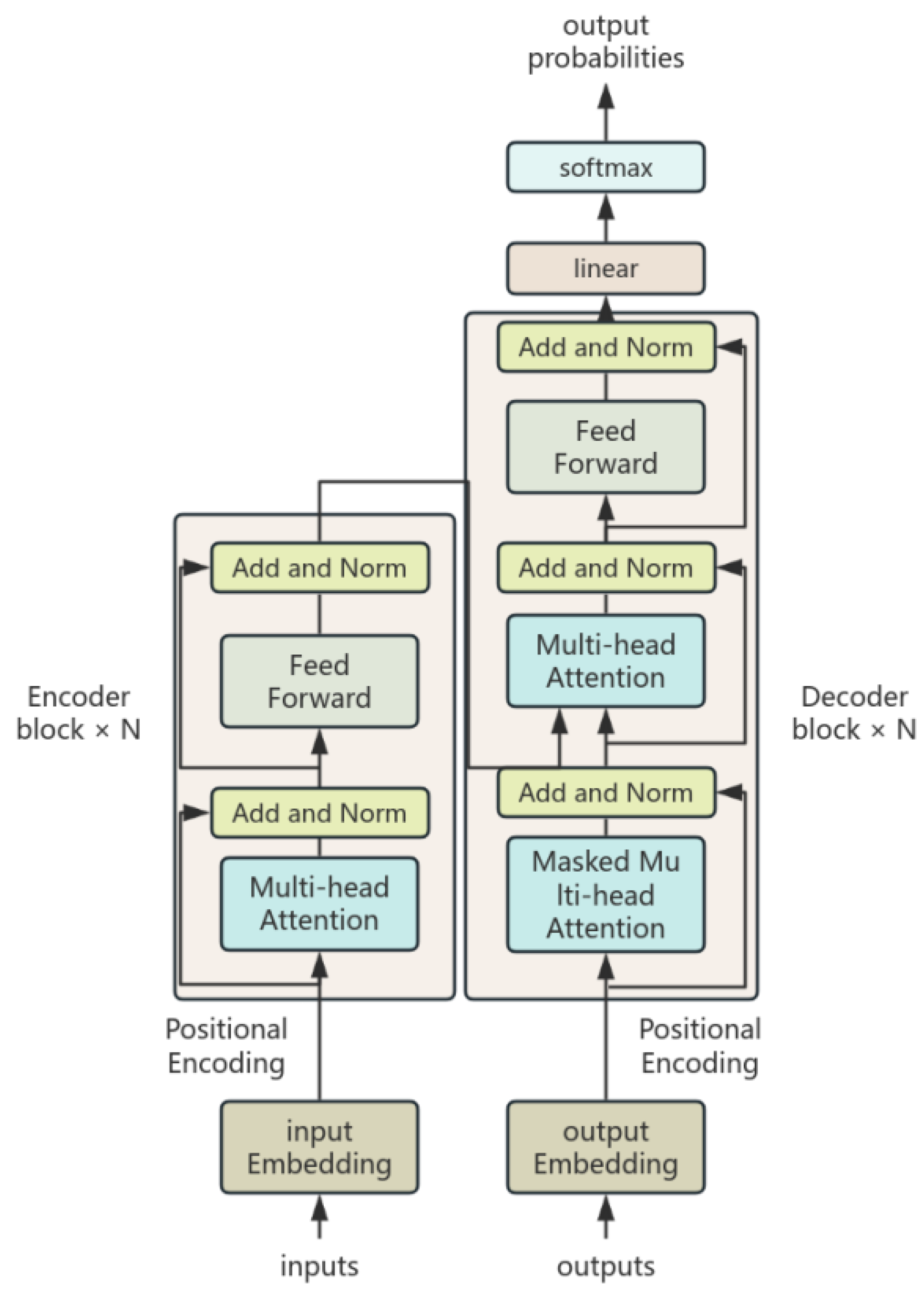
3.4.2. FT-Transformer

Although deep learning models are effective at tasks with unstructured data, such as computer vision (CV) and natural language processing (NLP), their application to tabular data presents several obstacles. FTT is a deep learning model that Gorishniy et al. proposed in 2021. It is designed to apply the Transformer [19] architecture to classification and regression tasks for tabular data [49].

FTT preprocesses tabular data by transforming it into a shape suitable for the Transformer via the Feature Tokenizer (FT) component and adding a classification token (CLS token) for training. FTT employs the same attention mechanism as the original Transformer, allowing the model to capture precise feature correlations while improving performance. Notably, empirical studies have validated its effectiveness in classification and regression benchmarks, including the California Housing (CA, real estate data), Adult (AD, income estimation), and Helena (HE, anonymized dataset) datasets, where it consistently outperformed traditional deep learning models [42]. Consequently, FTT is positioned as a standalone architecture that exhibits robustness across diverse application domains and offers a novel perspective on applying deep learning models to tasks involving tabular data.

The form of FTT significantly differs from typical CNN and RNN and is based on the encoder–decoder architecture. The encoder and decoder are made up of Multi-head attention layers and Feedforward Neural Networks (FNNs) [50]. The asymmetric network structure of the model is shown in Figure 2.

The attention mechanism is the main component of the Transformer. Its design resembles the visual attention mechanism of humans, in which a person prefers to focus more on the part that satisfies his or her demands while observing. The attention mechanism achieves this by adjusting the weight parameter, and the attention value is calculated by the following equation:

$$Attention(Q,K,V)=soft\max ({\displaystyle \frac{Q{K}^T}{\sqrt{d_k}}})V$$

(12)

where K, V, and Q signify the key matrix, value matrix, and query matrix, respectively, which are derived from the inputs by linear layer mapping, and d_k denotes the feature dimension of the Key vectors. The attention mechanism evaluates the similarity between K and V to derive the weight coefficients of each K and then obtains the attention values by multiplying the weights with V.

Multi-head attention is defined as the integration of h distinct attention mechanisms, with various output matrices spliced to produce the final output.

FTT further introduces the CLS token and FT on the basis of the Transformer. Figure 3 shows the structure of FTT.

FT encodes both categorical and numerical features into vectors so that more effective features can be extracted from tabular data. The encoding equation is as follows:

$$T_J^{(num)}=b_j^{(num)}+x_j^{(num)}{W}_j^{(num)}$$

(13)

$$T_J^{(cat)}=b_j^{(cat)}+e_j^T{W}_j^{(cat)}$$

(14)

$$T=stack\left[T_1^{(num)},\dots ,T_p^{(num)},T_1^{(cat)},\dots ,T_q^{(cat)}\right]$$

(15)

Then, T is integrated with the embedding layer of the CLS token using Equation (15). In this process, all feature information is added to the CLS token, which serves as the input to the transformer layer T₀. The process is shown as follows:

$$T_0=stack\left[[CLS],T\right]$$

(16)

$$T_i=F_i\left(T_{i-1}\right)$$

(17)

After stacking L layers of transformers, the CLS token can be extracted from the final output T_L and then passed to the prediction layer and used for the outcome. The process can be shown in Equation (18).

$$\stackrel{⌢}{y}=Linear(ReLU(LayerNorm(T_L^{\left[CLS\right]})))$$

(18)

In addition, the FTT removes the LayerNorm from the original Transformer input to improve the accuracy.

3.4.3. BO–FTT

In this paper, we propose an optimized model, BO–FTT, by tuning the main hyperparameters of FTT using the BO algorithm.

One of the essential components of the BO–FTT hybrid model is the iterative process of the BO algorithm. The approach first defines a parameter space and randomly selects a set of initial parameters to train and evaluate the FTT. The evaluated parameters are used to train the surrogate model that can predict the objective function value for any point in the parameter space. After that, the EI equation is used to select new parameters for evaluation, and the BO algorithm iteratively updates the surrogate model and gradually approaches the optimal parameters until the maximum number of iterations is reached.

The specific procedure for tuning the parameters of FTT using the BO algorithm is as follows:

• The objective function was configured as accuracy with init_points = 12, n_iter = 15, and a random seed of 1234. In addition, the five key parameters selected in this paper include core structural parameters, input_embed_dim, num_attn_blocks, and num_heads, and regularization parameters, attn_dropout and ff_dropout. Among them, num_heads determines the diversity of the multi-attention mechanism; input_embed_dim determines the vector representation capability of categorical features, which directly affects the model’s ability to capture feature differences; num_attn_blocks controls the model depth, where increased layers enhance feature interactions but heighten overfitting risks; attn_dropout can control the sparsity of the attention matrix through randomly masking some attention connections to prevent overfitting; ff_dropout is mainly used to regulate the overfitting risk of the feedforward network. The parameters and their value ranges are shown in

  Table 1. Parameters selected to be optimized in FTT and their value ranges.

  Parameter	Value Range
  num_heads (int)	(0, 10)
  num_attn_blocks (int)	(0, 10)
  input embed dim (int)	(0, 100)
  attn_dropout (float)	(0.1, 0.5)
  ff_dropout (float)	(0.1, 0.5)

  .

2.

Randomly select a set of parameters as initial evaluation points and compute the objective function values

3.

Use the current surrogate model and acquisition function to choose the next most promising site for sampling and assessing accuracy. Add the new observation point to the training data, and then update the surrogate model.

4.

Repeat the sampling, evaluation, updating, and checking process from Step 3 until either the maximum number of iterations of 100 times is reached or there is no improvement in the model’s accuracy within 20 iterations. At the end of each loop, output the parameters that maximize the accuracy of FTT.

The flow diagram of BO–FTT is shown in Figure 4.

The optimal parameters of the FTT are presented in

Table 2. Parameter settings of BO–FTT.

Parameter	Value
num_heads (int)	7
num_attn_blocks (int)	8
input embed dim (int)	77
attn_dropout (float)	0.21
ff_dropout (float)	0.20

.

4. Results

The analysis is conducted by classifying the preprocessed dataset using BO–FTT, and comparative experiments are designed to evaluate the performance of different models. We employed a Windows operating system and configured an environment with Python 3.11, while leveraging an NVIDIA GeForce RTX 4060 graphics processing unit (GPU) to accommodate the computing requirements.

The metrics used in experiments are listed below:

• Accuracy

Accuracy refers to the proportion of correctly classified samples to the total number of samples. The equation is as follows:

$$\mathrm{Accuracy}={\displaystyle \frac{\mathrm{TP}+\mathrm{TN}}{\mathrm{TP}+\mathrm{FP}+\mathrm{TN}+\mathrm{FN}}}$$

(19)

2.

Recall

Recall measures the proportion of actual positive samples that are correctly predicted as positive. The equation is as follows:

$$\mathrm{Recall}={\displaystyle \frac{\mathrm{TP}}{\mathrm{TP}+\mathrm{FN}}}$$

(20)

3.

Precision

Precision measures the proportion of samples predicted as positive that are actually positive. The equation is as follows:

$$\mathrm{Precision}={\displaystyle \frac{\mathrm{TP}}{\mathrm{TP}+\mathrm{FP}}}$$

(21)

4.

F1 score

F1 score takes into account both the recall and precision of the classification model. The range of the F1 score is (0,1), and the larger the value means the better performance. The equation is as follows:

$$F1=2\cdot {\displaystyle \frac{\mathrm{Precision}\cdot \mathrm{Recall}}{\mathrm{Precision}+\mathrm{Recall}}}$$

(22)

5.

AUC-ROC curve

The ROC curve depicts the relationship between the True Positive Rate (TPR) and the False Positive Rate (FPR). The area under the ROC curve (AUC) is used to quantify the performance of the ROC curve. Therefore, the AUC-ROC curve can comprehensively evaluate model performance in a situation of data imbalance and provide a more thorough assessment.

4.1. Performance Evaluation of BO–FTT

We trained the BO–FTT model, and its performance on the test set is shown in

Table 3. The performance of BO–FTT.

Evaluation Metrics	Value
Accuracy	91.81%
Precision	87.71%
Recall	89.10%
F1-score	88.37%

and Figure 5.

Table 3 demonstrates that the accuracy of BO–FTT reached 91.81%, indicating that the model can correctly predict 91.81% of RA patients and non-RA patients. Meanwhile, the model achieved an 87.71% in precision, 89.10% in recall, and 88.37% in F1 score, all of which showed that the model has produced feasible prediction results.

Meanwhile, Figure 5 shows that the AUC value in the test set was 0.89, with a 95% confidence interval of (0.845, 0.921). This indicated that the model demonstrates strong robustness and is capable of diagnosing the majority of RA patients when used to assist in the management of CKD patients. The ROC curve was near the upper left corner of the coordinate axis, indicating that the model could maintain a low FPR while producing a high TPR.

The accuracy of BO–FTT model on the training set and validation set with the number of iterations is shown in Figure 6. As shown, BO–FTT stabilized on the training set after approximately 21 iterations and achieved a peak accuracy of 91.81% at the 41st iteration on the validation set.

To further comprehend the predictive performance of BO–FTT, the confusion matrix [51] of the classification results was plotted. The confusion matrix is an effective visualization technique used mostly in supervised learning to compare classification results with actual values. Different columns in the confusion matrix represent the different predicted classes, and the total number of columns corresponds to the number of classes predicted by the model. Each row, on the other hand, represents the true classes of the samples, and the total number of rows corresponds to the number of actual classes. The confusion matrix of BO–FTT is shown in Figure 7.

Figure 7 shows that the number at (0, 0) was 496, indicating that 532 of the 496 positive samples were properly predicted. The result demonstrates that the BO–FTT model is capable of making accurate predictions for the majority of samples.

4.2. Comparative Experiments

To validate the efficacy of the proposed BO–FTT model, we conducted a comparative analysis by applying BO to three benchmark models: tabnet, Kolmogorov–Arnold Networks (KAN), and Multilayer Perceptron (MLP). Among them, MLP is one of the most basic and widely used neural network structures. It employs a straightforward stacking of fully connected layers, exhibiting strong stability and predictability in various tasks, especially in tabular data analysis [52]. Tabnet is a deep learning architecture designed for tabular data, featuring a unique attention mechanism and sparse feature selection module. While maintaining model interpretability, tabnet achieves feasible predictions [53]. KAN introduces an innovative approach by replacing fixed activation functions with trainable univariate spline functions. These adaptive functions dynamically adjust during training, offering enhanced flexibility compared to conventional architectures [54]. Therefore, these three models can constitute a control group for evaluating model performance.

Table 4. Parameter settings for different ML models.

Model	Value
BO–FTT	‘input_embed_dim’: 77; ‘attn_dropout’: 0.21; ‘num_heads’: 7; ‘ff_dropout’: 0.20; ‘num_attn_blocks’: 8
BO–tabnet	‘cat_emb_dim_label’: 9; ‘mask_type_label’: softmax; ‘optimizer_params’: 0.03;
BO–MLP	‘alpha’: 0.02; ‘hidden_layer_sizes’: 402;
BO–KAN	‘grid_eps’: 0.03; ‘grid_range_max’: 6; ‘grid_range_min’: −6; ‘grid_size’: 8; ‘scale_base’: 0.23; ‘scale_noise’: 0.27; ‘scale_spline’: 2.11; ‘spline_order’: 8

shows the hyperparameter settings of the selected models after being optimized.

The experimental results after tuning the hyperparameters and training these models are shown in

Table 5. Comparative experimental results of different ML models.

Model	Accuracy	Precision	Recall	F1-Score
BO–FTT	91.81%	87.71%	89.10%	88.37%
BO–tabnet	79.16%	77.31%	78.79%	78.04%
BO–MLP	86.40%	85.84%	86.40%	85.99%
BO–KAN	83.90%	81.05%	73.90%	71.88%

.

Table 5 shows that the BO–FTT and BO–MLP achieved more than an 80% accuracy, precision, recall, and F1 score. Meanwhile, BO–KAN and BO–tabnet reached more than 70% in all metrics.

In order to further intuitively understand the effects and gaps of these ML models with the BO algorithm, the experimental results are plotted as a bar chart, which is shown in Figure 8. It can be seen that the BO–FTT model demonstrated the best performance across all evaluation metrics, slightly surpassing the BO–MLP, which ranked second in overall performance. The BO–KAN and BO–tabnet performed less effectively, although the BO–tabnet model, which obtained the lowest total rating, achieved more than 70% accuracy.

To demonstrate the significance of using the BO algorithm for parameter tuning in improving model performance, this work trained and evaluated the FTT model without parameter tuning and then compared the experimental results of FTT to BO–FTT. The experimental results are presented in

Table 6. Evaluation results of FTT.

Evaluation Metrics	Value
accuracy	88.01%
precision	82.35%
recall	83.83%
f1-score	83.05%

.

Table 5 shows that after being optimized by the BO algorithm, all model metrics showed an improvement, which means that tuning the parameters of FTT can indeed improve the performance of models to some extent.

To further validate the model’s reliability and generalizability, this study employed two public disease datasets—Breast Cancer Wisconsin [55] and Early Stage Diabetes Risk Prediction [56]—to assess the BO–FTT model’s predictive performance across distinct medical domains. The Breast Cancer Wisconsin dataset comprises 569 samples with 30 nuclear morphology features for classifying benign or malignant tumors, while the Early Stage Diabetes Risk Prediction dataset contains 520 samples with 16 clinical symptom indicators for binary classification of diabetes risk. Both datasets were pre-cleaned and balanced, requiring only normalization during preprocessing. The benchmark models, BO–MLP, BO–KAN, and BO–tabnet, were used for comparative analysis. The experimental results are presented in

Table 7. Performance of different ML models on Breast Cancer Wisconsin dataset.

Model	Accuracy	Precision	Recall	F1-Score
BO–FTT	96.49%	96.37%	96.01%	96.37%
BO–tabnet	94.74%	94.70%	94.70%	94.70%
BO–MLP	95.32%	95.37%	94.94%	95.14%
BO–KAN	92.41%	92.42%	91.00%	91.63%

and

Table 8. Performance of different ML models on Early Stage Diabetes Risk Prediction dataset.

Model	Accuracy	Precision	Recall	F1-Score
BO–FTT	97.12%	97.19%	96.81%	96.99%
BO–tabnet	87.65%	82.34%	83.11%	87.62%
BO–MLP	94.87%	94.84%	94.22%	94.51%
BO–KAN	87.50%	85.76%	85.17%	85.45%

.

As shown in Table 7 and Table 8, BO–FTT demonstrates superior performance in the prediction of diabetes and breast cancer, with accuracy rates reaching 96.49% and 97.12%. Its stable performance across differing pathological mechanisms and feature characteristics robustly confirms the model’s generalizability and exceptional predictive capability in diverse disease diagnostic tasks.

4.3. Interpretability of BO–FTT

In fields such as healthcare, the reliability of outcomes is highly critical, so the explainability of ML models has always been an important issue of concern for scholars. At the same time, due to the inherent complexity of the FTT model, understanding the reasons behind its decisions is also a key challenge. As a result, the gradient feature importances [57] were calculated and ranked for the BO–FTT model to determine the contribution of the features to the outcomes and to assess the interpretability of the model.

The overall explanation obtained for the model is shown in Figure 9. It can be seen that complications of metastatic solid tumors are one of the most important risk factors for anemia in CKD patients. This may be due to tumor-related inflammation, such as increased levels of interleukin-6 and tumor necrosis factor-α, which suppress red blood cell production and interfere with iron absorption. Additionally, tumor infiltration of the bone marrow directly destroys the hematopoietic microenvironment, creating a synergistic effect with the inherent lack of EPO in CKD, further exacerbating anemia [58]. Paraplegia is another significant factor for the occurrence of anemia in CKD patients. Patients with paraplegia may experience acute blood loss related to spinal cord injury, while chronic inflammation from pressure sores and urinary tract infections can suppress EPO production and iron metabolism, leading to anemia [59]. In diabetic patients, chronic inflammation can also increase hepcidin levels and inhibit iron absorption. Concurrently, renal impairment reduces EPO production, and metabolic disorders shorten the lifespan of red blood cells [60]. Liver disease patients often develop splenomegaly, which accelerates erythrocyte destruction through hemolysis, significantly increasing anemia risk [61].

Gender and age are also factors affecting the occurrence of anemia in RA. Female CKD patients may have a higher incidence and severity of anemia due to menstrual blood loss, increased iron demands during pregnancy, and hormonal changes after menopause; older CKD patients are at a significantly higher risk of anemia due to renal function decline, chronic inflammation, malnutrition, and multiple comorbidities [62].

The reduction in red blood cell count and hematocrit is an important manifestation of anemia, reflecting insufficient red blood cell production. Concurrently, the increase in white blood cell count and the absolute value of neutrophils indicate the presence of inflammation or infection in the body. This chronic inflammatory state can further exacerbate anemia by suppressing EPO production and disrupting iron metabolism. Furthermore, rising total bilirubin levels typically signal accelerated hemolysis. Potential mechanisms include direct inhibition of bone marrow hematopoietic function by unconjugated bilirubin, as well as indirect aggravation of anemia through hemoglobin degradation, which worsens iron dysregulation [63].

5. Discussion

This paper explains the design of a model to tune the hyperparameters of FTT using a BO algorithm and effectively completed an early prediction about the risk of anemia in patients with CKD. Compared to existing studies utilizing FTT or BO for medical prediction, this study employs three distinct feature selection methods based on different principles to enhance model efficiency and accuracy. Additionally, we conducted an interpretability analysis on the FTT to elucidate the relative importance of various features in model outputs, thereby identifying potential critical indicators influencing disease onset.

Medical records from the MIMIC database were extracted in this work. After preprocessing and feature selection, the dataset was fed into the BO–FTT model to predict whether a CKD patient had RA or not. The results showed that the BO–FTT achieved better results and more reliable predictions, outperforming the untuned FTT model by 3.8% in accuracy and outperforming BO–tabnet, BO–MLP, and BO–KAN in terms of all evaluation metrics. Therefore, we hope that this optimized BO–FTT model can become a part of the clinical decision support system, assisting doctors in identifying high-risk groups potentially suffering from RA early in the management of CKD patients. The proposed BO–FTT not only enables more timely preventive or interventional measures to delay disease progression and improve patient outcomes, but also provides a lightweight algorithmic solution for portable medical electronic devices, filling the critical gap in real-time RA prediction within electronic health systems.

In the future, the model will be upgraded to accommodate increasingly complex disease diagnoses. For instance, besides hyperparameter optimization, adjustments to the structure of FTT, such as optimizing the attention mechanism, could be considered. In addition, we will investigate whether there are suitable ensemble methods that can achieve more effective predictions while maintaining high efficiency and providing robust interpretability analysis.

References

1. Pramod, S.; Goldfarb, D.S. Challenging patient phenotypes in the management of anemia of chronic kidney disease. Int. J. Clin. Pract. 2021, 75, e14681. [Google Scholar] [CrossRef] [PubMed]
2. Comini, L.D.O.; de Oliveira, L.C.; Borges, L.D.; Dias, H.H.; Batistelli, C.R.S.; Ferreira, E.D.S.; da Silva, L.S.; Moreira, T.R.; da Costa, G.D.; da Silva, R.G.; et al. Prevalence of chronic kidney disease in Brazilians with arterial hypertension and/or diabetes mellitus. J. Clin. Hypertens. 2020, 22, 1666–1673. [Google Scholar] [CrossRef] [PubMed]
3. Gansevoort, R.T. Too much nephrology? The CKD epidemic is real and concerning. A PRO view. Nephrol. Dial. Transplant. 2019, 34, 577–580. [Google Scholar] [CrossRef] [PubMed]
4. Smemr, A.; Hallmark, B.F. Complications of Kidney Disease. Nurs. Clin. N. Am. 2018, 53, 579–588. [Google Scholar]
5. Pazianas, M.; Miller, P.D. Osteoporosis and chronic kidney disease–mineral and bone disorder (CKD-MBD): Back to basics. Am. J. Kidney Dis. 2021, 78, 582–589. [Google Scholar] [CrossRef]
6. Farinha, A.; Mairos, J.; Fonseca, C. Anemia in Chronic Kidney Disease: The State of the Art. Acta Medica Port. 2022, 35, 758–764. [Google Scholar] [CrossRef]
7. Odawara, M.; Nishi, H.; Nangaku, M. A spotlight on using HIF-PH inhibitors in renal anemia. Expert Opin. Pharmacother. 2024, 25, 1291–1299. [Google Scholar] [CrossRef]
8. Figurek, A.; Rroji, M.; Spasovski, G. FGF23 in chronic kidney disease: Bridging the heart and anemia. Cells 2023, 12, 609. [Google Scholar] [CrossRef]
9. Fishbane, S.; Pollock, C.A.; El-Shahawy, M.; Escudero, E.T.; Rastogi, A.; Van, B.P.; Frison, L.; Houser, M.; Pola, M.; Little, D.J.; et al. Roxadustat versus epoetin alfa for treating anemia in patients with chronic kidney disease on dialysis: Results from the randomized phase 3 ROCKIES study. J. Am. Soc. Nephrol. 2022, 33, 850–866. [Google Scholar] [CrossRef]
10. Guzzo, I.; Atkinson, M.A. Anemia after kidney transplantation. Pediatr. Nephrol. 2023, 38, 3265–3273. [Google Scholar] [CrossRef]
11. Cui, J.; Yang, J.; Zhang, K.; Xu, G.; Zhao, R.; Li, X.; Liu, L.; Zhu, Y.; Zhou, L.; Yu, P.; et al. Machine learning-based model for predicting incidence and severity of acute ischemic stroke in anterior circulation large vessel occlusion. Front. Neurol. 2021, 12, 749599. [Google Scholar] [CrossRef] [PubMed]
12. Bahrainwala, J.; Berns, J.S. Diagnosis of iron-deficiency anemia in chronic kidney disease. Semin. Nephrol. 2016, 36, 94–98. [Google Scholar] [CrossRef] [PubMed]
13. Agoro, R.; Montagna, A.; Goetz, R.; Aligbe, O.; Singh, G.; Coe, L.M.; Mohammadi, M.; Rivella, S.; Sitara, D. Inhibition of fibroblast growth factor 23 (FGF23) signaling rescues renal anemia. FASEB J. 2018, 32, 3752. [Google Scholar] [CrossRef] [PubMed]
14. Tirmenstajn-Jankovic, B.; Dimkovic, N.; Perunicic-Pekovic, G.; Radojicic, Z.; Bastac, D.; Zikic, S.; Zivanovic, M. Anemia is independently associated with NT-proBNP levels in asymptomatic predialysis patients with chronic kidney disease. Hippokratia 2013, 17, 307. [Google Scholar]
15. el Din Afifi, E.N.; Tawfik, A.M.; Abdulkhalek, E.E.R.S.; Khedr, L.E. The relation between vitamin D status and anemia in patients with end stage renal disease on regular hemodialysis. J. Ren. Endocrinol. 2021, 7, e15. [Google Scholar] [CrossRef]
16. Kamei, D.; Nagano, M.; Takagaki, T.; Tomotaka, S.; Ken, T. Comparison between liquid chromatography/tandem mass spectroscopy and a novel latex agglutination method for measurement of hepcidin-25 concentrations in dialysis patients with renal anemia: A multicenter study. Heliyon 2023, 9, e13896. [Google Scholar] [CrossRef]
17. Akchurin, O.; Patino, E.; Dalal, V. Interleukin-6 contributes to the development of anemia in juvenile CKD. Kidney Int. Rep. 2019, 4, 470–483. [Google Scholar] [CrossRef]
18. Verma, A.; Jain, M. Predicting the Risk of Diabetes and Heart Disease with Machine Learning Classifiers: The Mediation Analysis. Meas. Interdiscip. Res. Perspect. 2024, 42, 1–18. [Google Scholar] [CrossRef]
19. Vaswani, A.; Shazeer, N.; Parmar, N.; Uszkoreit, J.; Jones, L.; Gomez, A.N.; Kaiser, L.; Polosukhin, I. Attention is all you need. Adv. Neural Inf. Process. Syst. 2017, 30. [Google Scholar]
20. Tomašev, N.; Glorot, X.; Rae, J.W. A clinically applicable approach to continuous prediction of future acute kidney injury. Nature 2019, 572, 116–119. [Google Scholar] [CrossRef]
21. Yue, S.; Li, S.; Huang, X. Machine learning for the prediction of acute kidney injury in patients with sepsis. J. Transl. Med. 2022, 20, 215. [Google Scholar] [CrossRef]
22. She, S.; Shen, Y.; Luo, K.; Zhang, X.; Luo, C. Prediction of Acute Kidney Injury in Intracerebral Hemorrhage Patients Using Machine Learning. Neuropsychiatr. Dis. Treat. 2023, 19, 2765–2773. [Google Scholar] [CrossRef] [PubMed]
23. Qu, C.; Gao, L.; Yu, X.; Wei, M.; Fang, G.Q.; He, J.; Li, W.Q. Machine learning models of acute kidney injury prediction in acute pancreatitis patients. Gastroenterol. Res. Pract. 2020, 2020, 3431290. [Google Scholar] [CrossRef] [PubMed]
24. Zhang, R.; Yin, M.; Jiang, A.; Zhang, S.; Xu, X.; Liu, L. Automated machine learning for early prediction of acute kidney injury in acute pancreatitis. BMC Med. Inform. Decis. Mak. 2024, 24, 16. [Google Scholar] [CrossRef] [PubMed]
25. Chang, H.L.; Wu, C.C.; Lee, S.P.; Chen, Y.K.; Su, W.; Su, S.L. A predictive model for progression of CKD. Medicine 2019, 98, e16186. [Google Scholar] [CrossRef]
26. Galloway, C.D.; Valys, A.V.; Shreibati, J.B.; Treiman, D.L.; Petterson, F.L.; Gundotra, V.P.; Friedman, P.A. Development and validation of a deep-learning model to screen for hyperkalemia from the electrocardiogram. JAMA Cardiol. 2019, 4, 428–436. [Google Scholar] [CrossRef]
27. Chittora, P.; Chaurasia, S.; Chakrabarti, P.; Kumawat, G.; Chakrabarti, T.; Leonowicz, Z.; Bolshev, V. Prediction of chronic kidney disease—A machine learning perspective. IEEE Access 2021, 9, 17312–17334. [Google Scholar] [CrossRef]
28. Song, W.; Zhou, X.; Duan, Q.; Wang, Q.; Li, Y.; Li, A.; Zhou, W.; Sun, L.; Qiu, L.; Li, R.; et al. Using random forest algorithm for glomerular and tubular injury diagnosis. Front. Med. 2022, 9, 911737. [Google Scholar] [CrossRef]
29. Swain, D.; Mehta, U.; Bhatt, A.; Patel, H.; Patel, K.; Mehta, D.; Acharya, B.; Gerogiannis, V.C.; Kanavos, A.; Manika, S. A robust chronic kidney disease classifier using machine learning. Electronics 2023, 12, 212. [Google Scholar] [CrossRef]
30. Zheng, J.X.; Li, X.; Zhu, J.; Guan, S.Y.; Zhang, S.X.; Wang, W.M. Interpretable machine learning for predicting chronic kidney disease progression risk. Digit. Health 2024, 10, 20552076231224225. [Google Scholar] [CrossRef]
31. Zhang, W.; Liu, X.; Dong, Z.; Wang, Q.; Pei, Z.; Chen, Y.; Zheng, Y.; Wang, Y.; Chen, P.; Feng, Z.; et al. New diagnostic model for the differentiation of diabetic nephropathy from non-diabetic nephropathy in Chinese patients. Front. Endocrinol. 2022, 13, 913021. [Google Scholar] [CrossRef] [PubMed]
32. Jiang, S.; Fang, J.; Yu, T.; Liu, L.; Zou, G.; Gao, H.; Zhuo, L.; Li, W. Novel model predicts diabetic nephropathy in type 2 diabetes. Am. J. Nephrol. 2020, 51, 130–138. [Google Scholar] [CrossRef] [PubMed]
33. Johnson, A.; Bulgarelli, L.; Pollard, T.; Horng, S.; Celi, L.A.; Mark, R. MIMIC-IV (version 2.0). PhysioNet 2022, 24, 49–55. [Google Scholar]
34. Aljrees, T. Improving prediction of cervical cancer using KNN imputer and multi-model ensemble learning. PLoS ONE 2024, 19, e0295632. [Google Scholar] [CrossRef]
35. Balaram, A.; Vasundra, S. Prediction of software fault-prone classes using ensemble random forest with adaptive synthetic sampling algorithm. Autom. Softw. Eng. 2022, 29, 6. [Google Scholar] [CrossRef]
36. Marcos-Zambrano, L.J.; Karaduzovic-Hadziabdic, K.; Loncar Turukalo, T.; Przymus, P.; Trajkovik, V.; Aasmets, O.; Berland, M.; Gruca, A.; Hasic, J.; Hron, K. Applications of machine learning in human microbiome studies: A review on feature selection, biomarker identification, disease prediction and treatment. Front. Microbiol. 2021, 12, 634511. [Google Scholar] [CrossRef]
37. Pudjihartono, N.; Fadason, T.; Kempa-Liehr, A.W.; O′Sullivan, J.M. A review of feature selection methods for machine learning-based disease risk prediction. Front. Bioinform. 2022, 2, 927312. [Google Scholar] [CrossRef]
38. Domingo, D.; Kareem, A.B.; Okwuosa, C.N.; Custodio, P.M.; Hur, J.W. Transformer Core Fault Diagnosis via Current Signal Analysis with Pearson Correlation Feature Selection. Electronics 2024, 13, 926. [Google Scholar] [CrossRef]
39. Zhou, S.; Li, T.; Li, Y. Recursive feature elimination based feature selection in modulation classification for MIMO systems. Chin. J. Electron. 2023, 32, 785–792. [Google Scholar] [CrossRef]
40. Zhang, G.; Zhao, W.; Sheng, Y. Variable selection for uncertain regression models based on elastic net method. Commun. Stat.-Simul. Comput. 2024, 49, 1–22. [Google Scholar] [CrossRef]
41. Cao, Y.; Li, B.; Xiang, Q.; Zhang, Y. Experimental Analysis and Machine Learning of Ground Vibrations Caused by an Elevated High-Speed Railway Based on Random Forest and Bayesian Optimization. Sustainability 2023, 15, 12772. [Google Scholar] [CrossRef]
42. Gorishniy, Y.; Rubachev, I.; Khrulkov, V.; Babenko, A. Revisiting deep learning models for tabular data. Adv. Neural Inf. Process. Syst. 2021, 34, 18932–18943. [Google Scholar]
43. Kumar, P.; Nair, G.G. An efficient classification framework for breast cancer using hyper parameter tuned Random Decision Forest Classifier and Bayesian Optimization. Biomed. Signal Process. Control 2021, 68, 102682. [Google Scholar]
44. Özkale, M.R.; Abbasi, A. Iterative restricted OK estimator in generalized linear models and the selection of tuning parameters via MSE and genetic algorithm. Stat. Pap. 2022, 63, 1979–2040. [Google Scholar] [CrossRef]
45. Liwei, T.; Li, F.; Yu, S.; Yuankai, G. Forecast of lstm-xgboost in stock price based on bayesian optimization. Intell. Autom. Soft Comput. 2021, 29, 855–868. [Google Scholar] [CrossRef]
46. Cavoretto, R.; De Rossi, A.; Lancellotti, S.; Romaniello, F. Parameter tuning in the radial kernel-based partition of unity method by Bayesian optimization. J. Comput. Appl. Math. 2024, 451, 116108. [Google Scholar] [CrossRef]
47. Snoek, J.; Larochelle, H.; Adams, R.P. Practical bayesian optimization of machine learning algorithms. Adv. Neural Inf. Process. Syst. 2012, 25, 2960–2968. [Google Scholar]
48. Williams, C.K.I.; Rasmussen, C.E. Gaussian Processes for Machine Learning; MIT Press: Cambridge, MA, USA, 2006. [Google Scholar]
49. Jaffari, Z.H.; Abbas, A.; Kim, C.M.; Shin, J.; Kwak, J.; Son, C.; Lee, Y.-G.; Kim, S.; Chon, K.; Cho, K.H. Transformer-based deep learning models for adsorption capacity prediction of heavy metal ions toward biochar-based adsorbents. J. Hazard. Mater. 2024, 462, 132773. [Google Scholar] [CrossRef]
50. Isomura, T.; Shimizu, R.; Goto, M. Optimizing FT-Transformer: Sparse Attention for Improved Performance and Interpretability. Ind. Eng. Manag. Syst. 2024, 23, 253–266. [Google Scholar]
51. Yu, Z.; Li, X.; Sun, L. A transformer cascaded model for defect detection of sewer pipes based on confusion matrix. Meas. Sci. Technol. 2024, 35, 115410. [Google Scholar] [CrossRef]
52. Joo, Y.; Namgung, E.; Jeong, H.; Kang, I.; Kim, J.; Oh, S.; Lyoo, I.K.; Yoon, S.; Hwang, J. Brain age prediction using combined deep convolutional neural network and multi-layer perceptron algorithms. Sci. Rep. 2023, 13, 22388. [Google Scholar] [CrossRef] [PubMed]
53. Joseph, L.P.; Joseph, E.A.; Prasad, R. Explainable diabetes classification using hybrid Bayesian-optimized TabNet architecture. Comput. Biol. Med. 2022, 151, 106178. [Google Scholar] [CrossRef] [PubMed]
54. Sulaiman, M.H.; Mustaffa, Z.; Mohamed, A.I.; Samsudin, A.S.; Rashid, M.I.M. Battery state of charge estimation for electric vehicle using Kolmogorov-Arnold networks. Energy 2024, 311, 133417. [Google Scholar] [CrossRef]
55. Street, W.N.; Wolberg, W.H.; Mangasarian, O.L. Nuclear feature extraction for breast tumor diagnosis. In Proceedings of the Biomedical Image Processing and Biomedical Visualization, San Jose, CA, USA, 29 July 1993; SPIE: Bellingham, WA, USA, 1993; Volume 1905, pp. 861–870. [Google Scholar]
56. Islam, M.M.F.; Ferdousi, R.; Rahman, S.; Bushra, H. Likelihood prediction of diabetes at early stage using data mining techniques. Adv. Intell. Syst. Comput. 2020, 992, 113–125. [Google Scholar]
57. Sterratt, D.C. On the importance of countergradients for the development of retinotopy: Insights from a generalised Gierer model. PLoS ONE 2013, 8, e67096. [Google Scholar] [CrossRef]
58. Frisbie, J.H. Anemia and hypoalbuminemia of chronic spinal cord injury: Prevalence and prognostic significance. Spinal Cord 2010, 48, 566–569. [Google Scholar] [CrossRef]
59. Bozzini, C.; Busti, F.; Marchi, G.; Vianello, A.; Cerchione, C.; Martinelli, G.; Girelli, D. Anemia in patients receiving anticancer treatments: Focus on novel therapeutic approaches. Front. Oncol. 2024, 14, 1380358. [Google Scholar] [CrossRef]
60. Mehdi, U.; Toto, R.D. Anemia, diabetes, and chronic kidney disease. Diabetes Care 2009, 32, 1320–1326. [Google Scholar] [CrossRef]
61. Singh, S.; Manrai, M.; Kumar, D.; Srivastava, S.; Pathak, B. Association of liver cirrhosis severity with anemia: Does it matter? Ann. Gastroenterol. 2020, 33, 272. [Google Scholar] [CrossRef]
62. Santos, S.; Lousa, I.; Carvalho, M.; Sameiro-Faria, M.; Santos-Silva, A.; Belo, L. Anemia in Elderly Patients: Contribution of Renal Aging and Chronic Kidney Disease. Geriatrics 2025, 10, 43. [Google Scholar] [CrossRef]
63. Tefferi, A.; Hanson, C.A.; Inwards, D.J. How to interpret and pursue an abnormal complete blood cell count in adults. In Mayo Clinic Proceedings; Elsevier: Amsterdam, The Netherlands, 2005; Volume 80, pp. 923–936. [Google Scholar]
Figure 1. The stages in the prediction of RA by BO–FTT.
Electronics 14 02471 g001
Figure 2. Transformer’s encoder–decoder structure with key components.
Electronics 14 02471 g002
Figure 3. The structure of FTT.
Electronics 14 02471 g003
Figure 4. The flow diagram of BO–FTT in prediction tasks.
Electronics 14 02471 g004
Figure 5. ROC curve of BO–FTT.
Electronics 14 02471 g005
Figure 6. The accuracy of BO–FTT on training and validation sets with the number of iterations. The red star denotes the peak validation accuracy.
Electronics 14 02471 g006
Figure 7. Confusion matrix of BO–FTT.
Electronics 14 02471 g007
Figure 8. Performance comparison of different ML models.
Electronics 14 02471 g008
Figure 9. Feature importances of BO–FTT.
Electronics 14 02471 g009