Article

MSGformer: A Hybrid Multi-Scale Graph–Transformer Architecture for Unified Short- and Long-Term Financial Time Series Forecasting

1
School of Computer Science and Technology, Henan Polytechnic University, Jiaozuo 454000, China
2
Hebi National Optoelectronic Technology Co, Ltd., Hebi 458000, China
*
Author to whom correspondence should be addressed.
Electronics 2025, 14(12), 2457; https://doi.org/10.3390/electronics14122457
Submission received: 19 May 2025 / Revised: 11 June 2025 / Accepted: 12 June 2025 / Published: 17 June 2025

Abstract

Forecasting financial time series is challenging due to their intrinsic nonlinearity, high volatility, and complex dependencies across temporal scales. This study introduces MSGformer, a novel hybrid architecture that integrates multi-scale graph neural networks (MSGNet) with Transformer encoders to capture both local temporal fluctuations and long-term global trends in high-frequency financial data. The MSGNet module constructs multi-scale representations using adaptive graph convolutions and intra-sequence attention, while the Transformer component enhances long-range dependency modeling via multi-head self-attention. We evaluate MSGformer on minute-level stock index data from the Chinese A-share market, including CSI 300, SSE 50, CSI 500, and SSE Composite indices. Extensive experiments demonstrate that MSGformer significantly outperforms state-of-the-art baselines (e.g., Transformer, PatchTST, Autoformer) in terms of MAE, RMSE, MAPE, and R2. The results confirm that the proposed hybrid model achieves superior prediction accuracy, robustness, and generalization across various forecasting horizons, providing an effective solution for real-world financial decision-making and risk assessment.

1. Introduction

Stock price prediction is a fundamental task in the financial domain, essential for investment strategies, risk management, and enhancing market efficiency [1]. Financial time series data are influenced by a multitude of factors such as macroeconomic conditions, investor sentiment, and regulatory changes [2,3], leading to their inherently nonlinear and complex nature. Accurately forecasting stock trends remains a significant challenge.
Over the years, various traditional machine learning techniques have been employed to address the stock price prediction problem, such as support vector machines (SVMs) [4], decision trees [5], and k-nearest neighbors (KNNs) [6]. While these methods have provided valuable insights and demonstrated effectiveness in certain cases, they face significant limitations in the context of complex financial markets. Specifically, traditional machine learning approaches struggle with effectively balancing short-term volatility and long-term trends in time series forecasting [7,8]. To overcome this challenge, developing hybrid models that can simultaneously capture short-term local fluctuations and long-term global evolutionary features has emerged as a critical breakthrough direction for improving the accuracy of financial time series forecasting.
With the development of deep learning, more complex models have emerged, successfully capturing the nonlinear features in financial data. Among these, long short-term memory networks (LSTMs) [9], convolutional neural networks (CNNs) [10], and recurrent neural networks (RNNs) [11] have proven particularly effective for time series forecasting. However, when modeling both short-term fluctuations and long-term trends in financial time series, traditional deep learning architectures have their limitations: CNNs may lose important sequence information when extracting local features, while RNN models often suffer from vanishing or exploding gradients, limiting their ability to model long sequences [12]. The Transformer architecture was introduced to address these issues. Unlike CNNs and RNNs, the Transformer uses a self-attention mechanism to capture global dependencies in sequences and can process all elements of a sequence in parallel. This attention mechanism has achieved great success in natural language processing (NLP) [13] and has been extended to applications in computer vision [14], audio processing [15], and chemical sequence modeling [16]. These advancements suggest that the Transformer architecture holds great potential for financial time series modeling, especially in identifying long-term dependencies and complex interaction patterns.
Recent studies have confirmed this potential. For example, Zeng et al. (2023) evaluated various Transformer architectures and demonstrated their effectiveness in time series forecasting, particularly with the introduction of lightweight attention mechanisms [17]. Nie et al. (2024) provided a comprehensive survey of large language models and Transformer variants applied to financial data, highlighting their capacity to model market dynamics [18]. Moreover, TimesNet (Wu et al., 2022) and FEDformer (Zhou et al., 2021) have shown promising results in capturing both short- and long-term dependencies in high-frequency financial data [19,20]. These findings support the feasibility of using advanced Transformer-based architectures for financial forecasting tasks.
However, in the financial domain, most current applications of Transformers are still focused on text analysis, such as news or social media sentiment analysis, to indirectly predict market movements [21]. It is only recently that research has directly applied Transformers to stock price time series forecasting. However, applying the standard Transformer to multivariate stock prediction remains challenging, particularly when handling long historical sequences, as the computational cost is high and the original attention mechanism struggles to capture multi-scale patterns and suppress noise in financial data [18,22]. Therefore, there is an urgent need to design a novel architecture that efficiently handles long sequences and integrates diverse market information to enhance prediction performance [23].
A recent new model, multi-scale graph neural networks (MSGNet) [24], is a complex deep learning framework designed to handle multi-scale data, capturing local dynamics and broader market trends. Its primary strength lies in representing financial time series as a graph structure, with data points from different time scales acting as nodes linked by edges. This graph-based representation allows the model to effectively learn hierarchical structures and relationships within financial data, capturing complex multi-scale interactions. However, while MSGNet excels at handling high-dimensional financial data, it faces challenges in modeling long-term dependencies due to the limitations of its message-passing mechanism, which may not effectively capture global trends, limiting its ability to fully detect long-term changes in large-scale time series. To address the aforementioned challenges, this paper proposes MSGformer, a hybrid architecture that integrates multi-scale feature modeling with the sequential learning capability of Transformer. MSGformer combines the advantages of multi-scale graph neural networks (MSGNet) and Transformer, aiming to improve the accuracy of stock price prediction. In this model, the self-attention mechanism of Transformer is particularly effective in capturing long-term dependencies, especially global information across extended time scales. By integrating these two models, we leverage their complementary strengths to enhance both short-term and long-term forecasting of financial time series. The main contributions of this hybrid approach are summarized as follows.
  • We developed MSGformer to forecast financial time series, effectively capturing short-term volatility and long-term dependencies in market data;
  • To address the challenges of capturing local short-term dependencies in high-dimensional financial data, we incorporated a multi-scale graph neural network (MSGnet) to model complex market dynamics at multiple scales, improving the model’s ability to handle varied time resolutions;
  • By combining MSGnet’s ability to handle multi-dimensional data and Transformer’s attention mechanism, the proposed model overcomes the limitations of single-model approaches, achieving improved prediction accuracy across different financial forecasting tasks.
This paper is organized as follows: Section 2 reviews the related work. Section 3 introduces the model used in the article. Section 4 introduces the experiment. Section 5 presents the conclusion of this article.

2. Related Work

2.1. Traditional Methods

In early research, financial time series prediction mainly relied on econometric or statistical methods. The autoregressive integrated moving average model (ARIMA) and its enhancements are effective approaches for addressing this issue in econometrics and statistics [25]. Subsequently, ARIMA has been applied to time series forecasting in finance, resulting in several enhanced algorithms, including autoregressive (AR) [26], vector autoregressive (VAR) [27], autoregressive distributed lag (ARDL) [28], autoregressive conditional heteroskedasticity (ARCH) [29], generalized ARCH (GARCH) [30], and mixed data sampling (MIDAS) [31]. Although these techniques can be successfully used for short-term prediction, they are not suitable for nonlinear problems and have poor long-term prediction performance [32,33]. In order to solve this problem, machine learning is introduced to analyze time series and successfully applied to stock price forecasting [34,35]. Research indicates that machine learning algorithms, through adaptive noise suppression mechanisms such as regularization constraints and feature importance weighting, can effectively separate high-frequency noise from underlying signals in financial time series, thereby capturing the inherent nonlinear correlation patterns of data more accurately and significantly improving the prediction accuracy [36]. Machine learning methods include support vector machine (SVM), decision tree, naive Bayes, random forest, and so on. Wang et al. (2013) used a hybrid model of decision tree and SVM to predict future price trends [37]. IK Nti et al. (2020) established a feature-weighted SVM and k-nearest neighbor algorithm to predict the stock market index [38]. Avraam Tsantekidis et al. (2017) used convolutional neural networks for stock price prediction and found they outperformed multilayer perceptrons and support vector machines in predictive capability [39,40]. By leveraging large-scale financial datasets, AI algorithms can identify complex nonlinear patterns and subtle market signals that are often overlooked by traditional methods. This capability enables more accurate stock price forecasting, early detection of market trends, and data-driven investment strategies that enhance portfolio performance [41,42,43,44].

2.2. Deep Learning Approaches

Deep learning technology has been extensively utilized in the field of financial time series prediction, particularly in the context of short-term prediction tasks. A significant number of studies have focused on the capture of short-term market volatility and temporary market sentiment changes through models such as deep neural networks (DNNs), convolutional neural networks (CNNs), and long-term and short-term memory networks (LSTMs). In the study conducted by Wu et al. (2022), the utilization of the LSTM network proved to be a successful method for predicting short-term fluctuations in stock prices [19]. Wan A. et al. (2023) further enhanced the prediction accuracy by integrating the convolutional neural network (CNN) and the long short-term memory (LSTM) algorithms. These methods have been shown to exhibit enhanced resilience to short-term dependencies and rapid responsiveness to market fluctuations [45].

2.3. Transformer Methods

Despite the Transformer model’s extensive adoption and its proven efficacy in numerous sequential modeling tasks, its utilization in time series forecasting remains constrained by several significant limitations. Firstly, the self-attention mechanism of the Transformer exhibits quadratic computational complexity with respect to sequence length. This results in substantial computational resource consumption and reduced scalability when processing long sequences [17]. Secondly, the fixed positional encoding employed by the traditional Transformer is inadequate in effectively representing the periodic patterns that are commonly observed in time series data. This limitation restricts the model’s capacity to capture complex temporal dependencies [46]. Consequently, there is a necessity to develop structural optimizations and methodological enhancements to address the shortcomings of Transformer in terms of computational efficiency, temporal modeling capabilities, and robustness against noise, thereby improving its applicability to time series forecasting tasks.
In recent years, a series of Transformer-based architectures have been proposed specifically for time series forecasting tasks, addressing some of the computational and modeling limitations of the vanilla Transformer. For instance, Informer introduced the ProbSparse self-attention mechanism to reduce the complexity of long-sequence modeling while preserving forecasting accuracy [21]. Autoformer and FEDformer improved long-term series forecasting by incorporating trend-seasonal decomposition and frequency domain enhancements, respectively, which are particularly suitable for capturing periodic patterns in financial time series [20,46]. PatchTST leveraged a non-recurrent, convolution-free design by operating on time series patches with linear projections, demonstrating strong performance on high-frequency datasets [47]. Meanwhile, ETSformer integrated exponential smoothing principles into Transformer design to explicitly capture level, trend, and seasonality components [48].
Building upon these advances, our proposed MSGformer uniquely combines multi-scale graph modeling and Transformer-based global attention, enabling it to capture both short-term volatility and long-term dependencies. This hybrid architecture leverages insights from recent Transformer improvements while introducing novel multi-scale representations tailored to the financial domain.

3. Methodology

3.1. MSGNet

MSGNet is a new framework designed to capture the correlation between different sequences on different time scales. The whole model architecture is shown in Figure 1. MSGNet consists of multiple ScaleGraph blocks, the essence of which is that it can insert various components seamlessly. Each ScaleGraph block requires the following four-step sequence.
  • Identify the scale of the input time series;
  • Use adaptive graph convolution blocks to reveal the inter-sequence correlation of scale links;
  • Capture intra-sequence correlation through multi-head attention;
  • Use the SoftMax function to adaptively aggregate representations from different scales.
Figure 1. MSGNet employs several ScaleGraph blocks, each encompassing three pivotal modules: an FFT module for multiscale data identification, an adaptive graph convolution module for inter-series correlation learning within a time scale, and a multi-head attention module for intra-series correlation learning.
Electronics 14 02457 g001

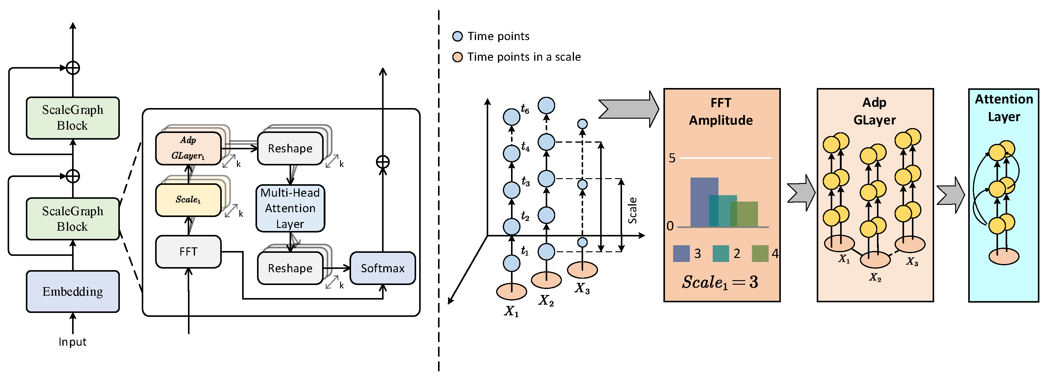
3.1.1. Scale Identification

Dominant time scales are extracted using Fast Fourier Transform (FFT):
F = A v g A m p F F T X e m p , f 1 , , f k = a r g T o p k F f * 1 , , L 2 , s i = L f i
Here, F F T and A m p denote the F F T and the calculation of amplitude values, respectively. The vector F ∈ L represents the calculated amplitude of each frequency, which is averaged across d m o d e l dimensions by the function A v g .
Based on the selected time scale s 1 , , s k , the input is reshaped into a 3D tensor by using the following equation to obtain multiple representations corresponding to different time scales:
X i = Re s h a p e s i , f i P a d d i n g X i n , i 1 , , k
To ensure uniform length across input time series, we initially used zero-padding. However, in this work, we further experimented with classical imputation techniques (e.g., linear interpolation and forward filling) to replace missing or extended values. These methods better preserve the underlying trends and reduce the risk of introducing artificial discontinuities.

3.1.2. Adaptive Graph Convolution

MSGNet proposes a novel multi-scale graph convolution method to capture specific and comprehensive inter-sequence dependencies. The specific methods are as follows.
Firstly, the tensor corresponding to the i-th scale is projected back to the tensor containing N variables by linear transformation, where N represents the number of time series. This projection is performed by the following defined linear transformation:
H i = W i X i
H i N × S I × f i , W i N × d m o d e l is a learnable weight matrix, tailored for tensors of the i-th scale.
In this method, the graph learning process involves generating two trainable parameters, E1 and E2. Then, by multiplying these two parameter matrices, an adaptive adjacency matrix is obtained according to the following formula:
A i = S o f t M a x Re L U E 1 i E 2 i T
After obtaining the adjacency matrix A i of the i-scale, the Mixhop graph convolution method is used to capture the correlation between sequences. Graph convolution is defined as follows:
H o u t i = σ | | j P A i j H i
H o u t i represents the output after the scale i fusion, σ() is the activation function, the hyperparameter P is a set of integer adjacent power, A i j represents the learned adjacency matrix A i multiplied by j times, and || represents the column-level connection, connecting the intermediate variables generated during each iteration.

3.1.3. Multi-Head Attention and Scale Aggregation
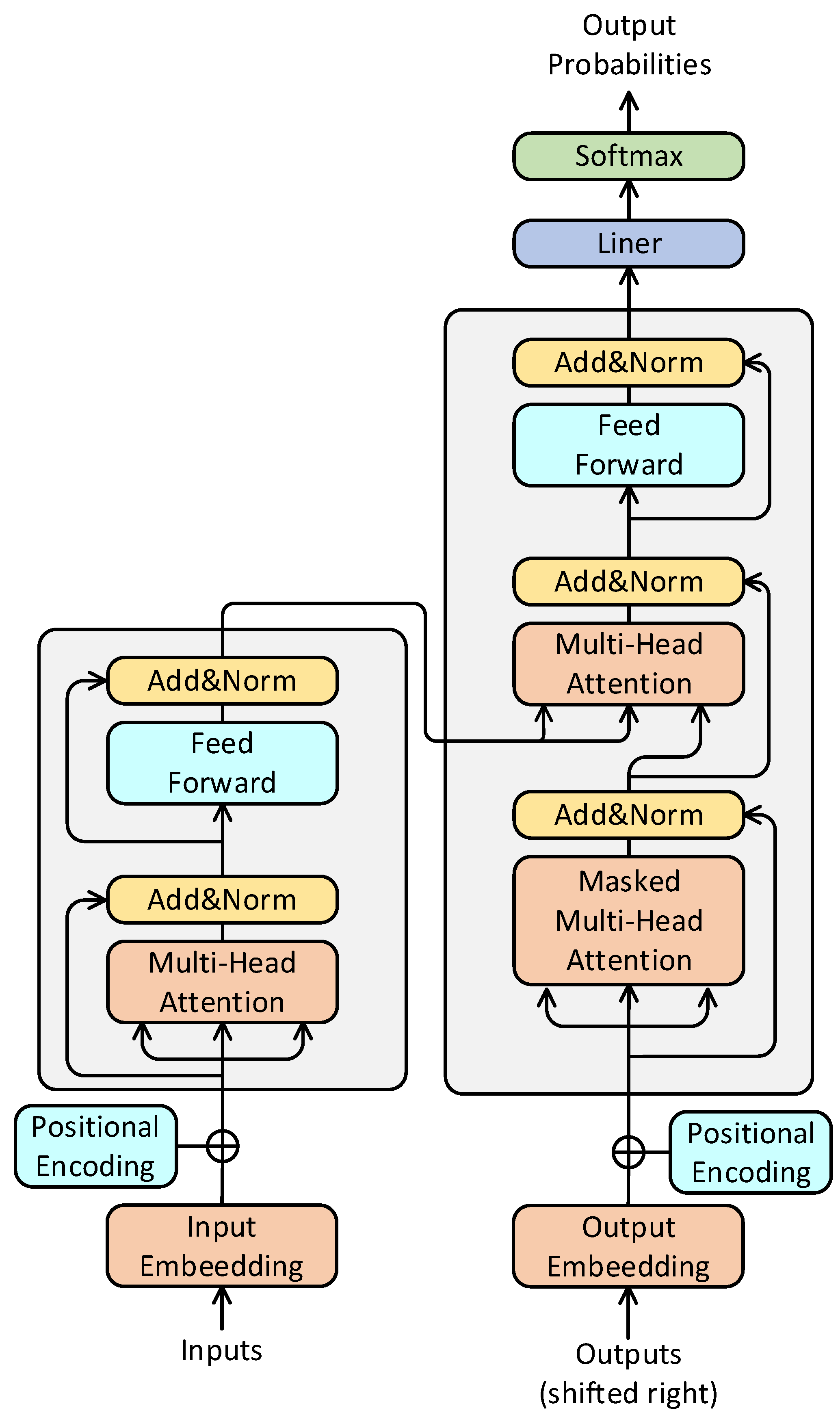
At each time scale, the multi-head attention (MHA) mechanism is used to capture the correlation within the sequence. Specifically, for the tensor χ ^ i of each time scale, the multi-headed attention mechanism of self-attention is applied on the time scale dimension of the tensor:
X ^ o u t i = M H A s X ^ i
M H A s refers to the multi-head attention function in the scale dimension proposed by Vaswani et al. (2017) [13]. In implementation, this involves reshaping the size of the input tensor from B × d m o d e l × s i × f i to the tensor of B f i × d m o d e l × s i , where B is the batch size.
Finally, for proceeding to the next layer, it is necessary to integrate k tensors X ^ o u t 1 , , X ^ o u t k of varying scales. Initially, each scale’s tensor is reshaped back into a two-dimensional matrix X ^ o u t i d m o d e l × L . Subsequently, the different scales are aggregated based on their amplitudes:
a ^ 1 , , a ^ k = S o f t M a x F f 1 , , F f k , X ^ o u t = i = 1 k a ^ i X ^ o u t i
F f 1 , , F f k is the amplitude corresponding to each scale, which is calculated by FFT. Then the SoftMax function is used to calculate the amplitude a ^ 1 , , a ^ k .

3.2. Transformer

Transformer is a deep learning architecture based on the self-attention mechanism. The core of its principle is to replace the traditional RNN and CNN with a self-attention mechanism to more efficiently capture long-range dependencies in sequence data. Transformer mainly consists of the following parts: a self-attention mechanism, multi-head attention mechanism, positional encoding, and encoder and decoder structure. The structure diagram of the Transformer is as follows (Figure 2).

3.2.1. Self-Attention

The self-attention mechanism is one of the core innovations of the Transformer model. Its purpose is to generate a weighted representation for each element by calculating the correlation between the elements of each position in the input sequence and the elements of all other positions. The calculation process of the self-attention mechanism can be divided into the following steps.
  • Query: Each input element is mapped into a query vector (Q);
  • Key: Each input element is also mapped to a bond vector (K);
  • Value: Each input element is mapped to a value vector (V).
Then, by calculating the similarity between the query vector and the key vector (usually using dot product or scaling dot product), an attention weight can be obtained. This weight is used to weight the value vector, and finally, a new representation is obtained. The formula of this process is as follows:
A t t e n t i o n Q , K , V = s o f t max Q K T d k V
Among them, d k is the dimension of the key vector, and the SoftMax function ensures that the sum of the ownership weights is 1, so that the model focuses on different parts of different positions in the sequence.

3.2.2. Multi-Head Attention

The multi-head attention mechanism in Transformer parallelizes the self-attention process by mapping the input queries, keys, and values into multiple subspaces. Self-attention is computed for each subspace, and the outputs are combined and linearly transformed to produce the final result. This approach allows the model to capture diverse relationships within the input sequence, enhancing its representational capacity.
As shown in Figure 3, the multi-head attention (MA) mechanism starts by applying scaled dot-product attention to the inputs V, Q, and K through linear transformations, computing each head separately. Although there are multiple heads with distinct parameters WWW for the linear transformations of Q, K, and V, it is collectively referred to as multi-head attention. Finally, the outputs of all heads are concatenated and linearly transformed to produce the final output of the MA mechanism.
The MA mechanism involves executing multiple self-attention operations on the initial input sequences V, Q, and K. Afterward, it concatenates the outcomes from each self-attention set and applies a single linear transformation to derive the final output. Specifically, its calculation formula is:
M u l t i H e a d Q , K , V = C i n c a t h e a d 1 , , h e a d h W o w h e r e   h e a d i = A t t e n t i o n Q W 1 Q , K W i Q , V W i V
The multi-head attention mechanism enables the model to focus on information from various subspaces at different positions, making it more effective than single self-attention.

3.2.3. Positional Encoding

Transformer introduces positional encoding, which enables the model to perceive the order of elements in the sequence by adding a position-related encoding to each input element. Position coding is usually generated by sine and cosine functions. The specific formula is:
P E p o s , 2 i = sin p o s 10,000 2 i / d m o d e l P E p o s , 2 i + 1 = cos p o s 10,000 2 i / d m o d e l
p o s is the location index, and d m o d e l denotes the embedding dimension. This encoding method can generate a different vector for each position, and the encoding of different positions can be combined with the input data in an additive form to help the model learn the relationship between positions.

3.2.4. Encoder and Decoder Structures

The Transformer model follows a typical encoder–decoder structure commonly used in sequence-to-sequence tasks like machine translation. The encoder is responsible for extracting features and learning representations of the input sequence. It consists of multiple identical layers, each containing a multi-head self-attention layer and a feed-forward neural network (FFN). The self-attention layer learns the relationships between each position in the input sequence, while the FFN transforms the representation of each position nonlinearly through two fully connected layers. To ensure stability and convergence during training, layer normalization and residual connections are applied to both the input and output of each layer.
The decoder generates the target sequence based on the encoder’s output. Similar to the encoder, it consists of multiple identical layers, but with an additional multi-head attention layer to compare the decoder’s output with the encoder’s output, aiding in generating the final prediction. The decoder’s structure mirrors the encoder, with self-attention and feed-forward networks, allowing it to produce the desired sequence by leveraging both the current input and the encoder’s learned representations.

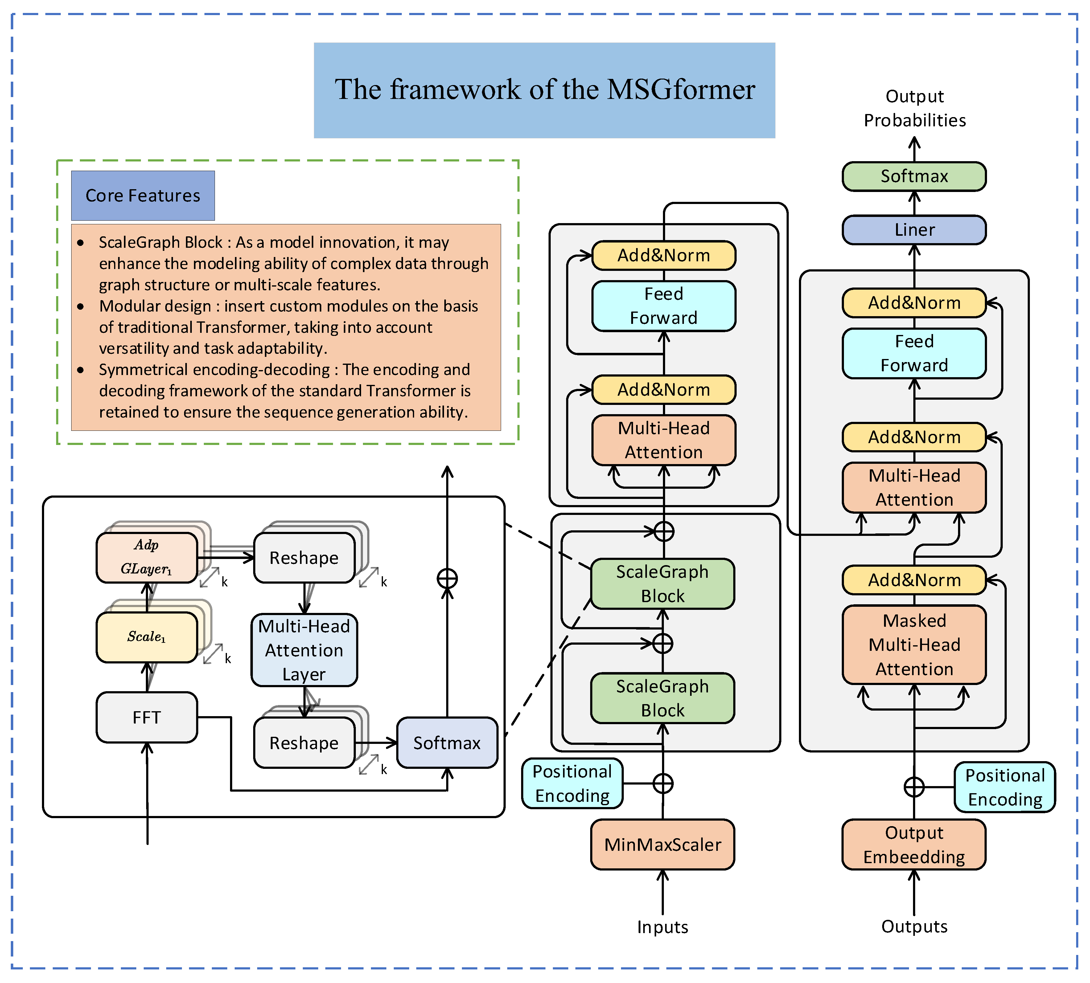
3.3. MSGformer Hybrid Model

The integration of MSGNet and Transformer in this study seeks to capitalize on the strengths of both models to address the complex challenges inherent in financial time series forecasting. MSGNet employs graph convolutional networks (GCNs) to process multi-scale data, thereby capturing local dynamics and multivariate relationships in financial time series. This renders it well-suited for handling heterogeneous data, such as prices and trading volumes. However, MSGNet is subject to limitations in terms of its capacity to capture long-term global dependencies and trends.
The incorporation of Transformer has been demonstrated to enhance the model’s capacity to capture global temporal dynamics. Transformer’s self-attention mechanism has been demonstrated to be effective in identifying global dependencies across extended time spans, particularly when dealing with long-term trends and macroeconomic influences. The combination of these two approaches enables the extraction of multi-scale features by MSGNet, which are then fed into Transformer to facilitate the capture of global trends and long-term dependencies through its self-attention mechanism. This enables the model to account for both short-term fluctuations and long-term trends, thereby improving prediction accuracy and robustness.
The integration of MSGNet’s local dependency modeling with Transformer’s global dependency modeling has been demonstrated to result in a more accurate and comprehensive forecasting capability for complex financial time series.

Structure of MSGformer

MSGformer combines the advantages of MSGNet and Transformer. In this model, the input data, which consist of multivariate time series (such as stock prices, trading volumes, and technical indicators), are first processed and normalized using MinMaxScaler to ensure that all features are within the same scale, facilitating more efficient model training. The data are then reshaped into a 3D format suitable for processing by the model.
The processed data are passed through MSGNet, where they are transformed into a graph structure. Each time step in the time series is represented as a node, and the relationships between different time steps are captured by graph edges. MSGNet then uses graph convolution and message passing mechanisms to extract multi-scale features from the data. These features represent both short-term fluctuations and long-term trends, allowing MSGNet to model the local dependencies within the time series at different temporal scales.
Once MSGNet has extracted the multi-scale features, they are passed to the Transformer encoder, where the self-attention mechanism of Transformer comes into play. The encoder uses multi-head self-attention to model long-range dependencies, enabling the model to capture global temporal patterns and understand the complex relationships between distant time steps. By considering interactions across all time steps, the self-attention mechanism enables the model to focus on key features relevant to long-term forecasting. Layer normalization and dropout are applied to improve the model’s stability and generalization.
Following the encoder, the data are passed to the Transformer decoder, which refines the learned representations from the encoder. The decoder uses a similar attention mechanism to the encoder, but this time, it also attends to the encoder’s output to further process the features and capture complex dependencies between different time steps. The final output is then passed through dense layers to generate the predicted values for future time steps. This output is shaped based on the required forecast horizon.
The model’s output is passed through a linear layer to generate the predictions, and the predictions are then inverse-normalized to bring them back to their original scale, making them suitable for real-world interpretation. By combining MSGNet’s capability to capture multi-scale features with Transformer’s ability to model long-term dependencies, MSGformer creates a robust framework that balances the capture of short-term volatility and long-term trends in financial time series prediction. This hybrid model allows for more accurate and stable predictions by leveraging the complementary strengths of both models. The structure of MSGformer model is shown in Figure 4.
The development of the MSGformer hybrid model was achieved through a meticulous process of model design and parameter tuning. The process prioritized the rationality of model architecture and parameter selection, thereby minimizing manual intervention while enhancing the model’s predictive performance and the clarity of parameter settings. The integration of the multi-scale graph neural network (MSGNet) with Transformer’s self-attention mechanism enables the model to efficiently handle the complexity of financial time series, thereby enhancing its robustness and accuracy. The system under discussion is especially effective in terms of balancing short-term fluctuations and long-term trends.

4. Experiments

In this study, both comparative and ablation experiments were conducted to evaluate the performance of MSGformer against other baseline models. The results demonstrate that MSGformer effectively captures short-term fluctuations and long-term dependencies in multivariate financial time series.
We selected four representative stock indices from the Chinese A-share market as forecasting targets: the CSI 300 Index, the SSE 50 Index, the CSI 500 Index, and the SSE Composite Index. These indices respectively represent large-cap stocks, blue-chip stocks, mid-cap stocks, and the overall market, providing high representativeness and practical significance. This selection enables the evaluation of the model’s generalization capability across different market structures.
The dataset comprises high-frequency 1 min trading data collected from January 2019 to December 2024, with over 600,000 data points. Due to its high density and complex temporal volatility, the dataset imposes significant challenges on the model’s learning ability. Each record includes features such as timestamp, open price, high price, low price, close price, and trading volume. The close price (Close) was selected as the primary target for prediction. Detailed software and hardware configurations used in the experiments are presented in Table 1.

4.1. Data Processing

The dataset underwent standardized preprocessing prior to use. We applied Z-score normalization, using the mean and standard deviation of the training set to normalize the entire dataset. This ensures that the model maintains consistent sensitivity to features with different numerical scales during training. Subsequently, a sliding window approach was adopted to construct the training samples, where a window length of T was set—using T consecutive time steps as input features to predict the stock price at T + 1.
To handle the variable lengths and incomplete sequences produced during sliding window construction, we initially used zero-padding to extend the sequences. However, we also explored classical imputation techniques such as linear interpolation and forward filling to fill in the extended parts of the sequences. These techniques better preserve the continuity and patterns of financial time series compared to zero-padding. Among them, linear interpolation was found to improve prediction robustness and was ultimately used in our final experiments.
Furthermore, to assess the model’s stability and generalization capability, the dataset was split into training (70%), validation (20%), and testing (10%) sets. All experiments were conducted under the same hardware environment to ensure fairness and reproducibility. The normalization formula is as follows:
x t = x t μ σ
where x ^ t is the normalized price at time t, and μ and σ are the sample mean and sample standard deviation of the training set.
In each forecast, this experiment uses the previous trading day’s closing price to predict the next trading day’s closing price + 1. A moving window is constructed by using the observed time series to construct functions and labels. Figure 5 shows the process in detail.
All reported experiments adopt a one-step-ahead forecasting horizon, corresponding to a 1 min ahead prediction. That is, given T minutes of historical data, the model is trained to predict the closing price at T + 1 min.
The current study focuses on high-frequency financial time series (1 min interval) to assess the model’s performance in capturing rapid market fluctuations. While MSGformer is theoretically adaptable to coarser granularities such as daily and monthly data, the model’s effectiveness at these resolutions remains an open question. We acknowledge that temporal scale can significantly affect model performance due to differences in noise levels, periodicity, and available context. As such, evaluating MSGformer on daily and monthly data is a valuable direction for future research.

4.2. Evaluation Criteria

To comprehensively evaluate the performance of the MSGformer model, four key metrics were employed: the coefficient of determination (R2), mean absolute error (MAE), root mean squared error (RMSE), and mean absolute percentage error (MAPE). These metrics provide complementary insights into the model’s predictive accuracy and its ability to capture both short-term fluctuations and long-term trends in stock prices.
R2 measures how well a regression model fits the data. An R2 value near 1 indicates a good fit, while a value near 0 suggests a poor fit. R2 is calculated as follows:
R 2 = 1 i = 1 n y ^ i y i 2 i = 1 n y i y ¯ 2
MAE is a metric that calculates the average absolute difference between predicted and actual values. It provides a straightforward measure of prediction accuracy, with smaller values indicating better model performance. MAE is calculated as follows:
M A E = 1 n i = 1 n | y ^ i y i |
RMSE is the square root of the mean of squared errors. Unlike MAE, RMSE penalizes larger errors more heavily due to the squaring process, making it particularly sensitive to outliers:
R M S E = 1 n i = 1 n y i y ^ i 2
MAPE expresses the average absolute error as a percentage of actual values, offering a scale-independent metric that is easy to interpret across different datasets:
M A P E = 100 % n i = 1 n y i y ^ i y i

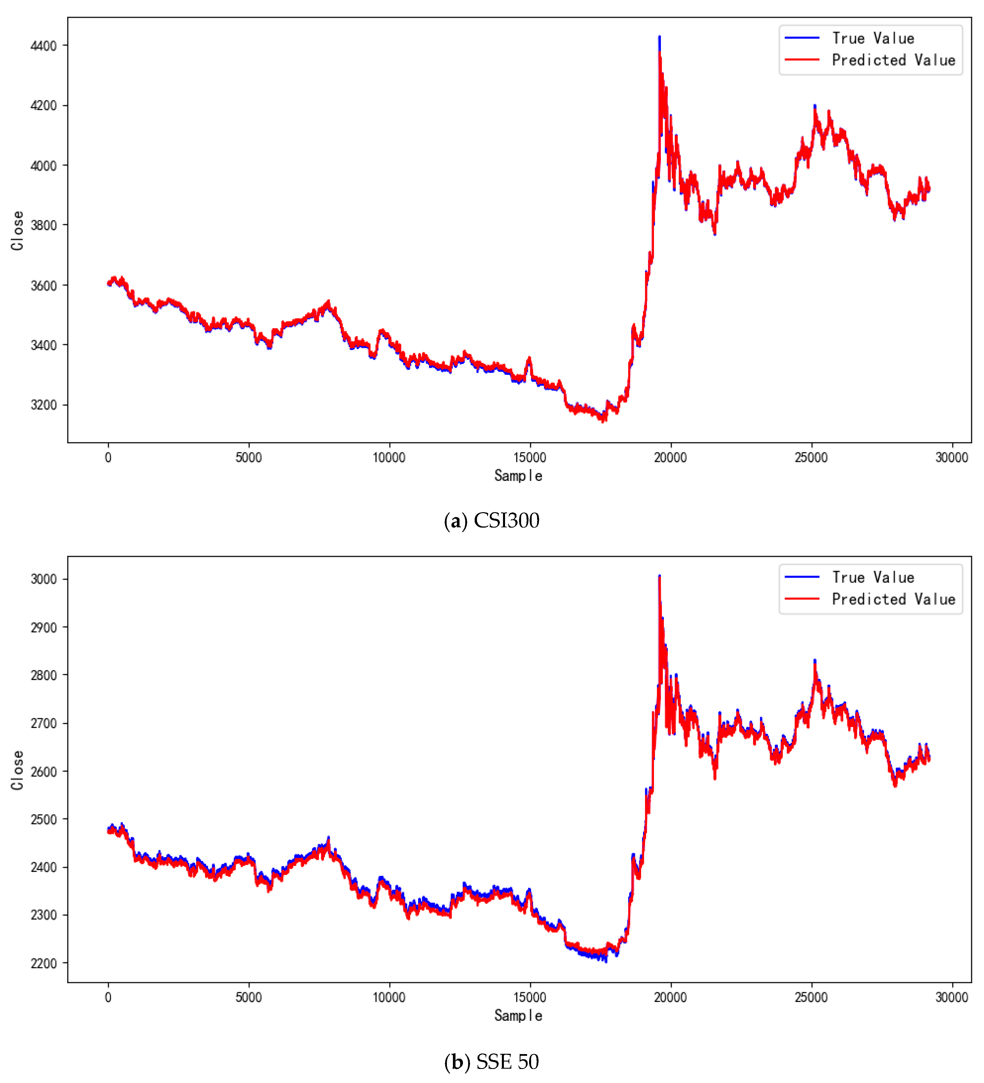
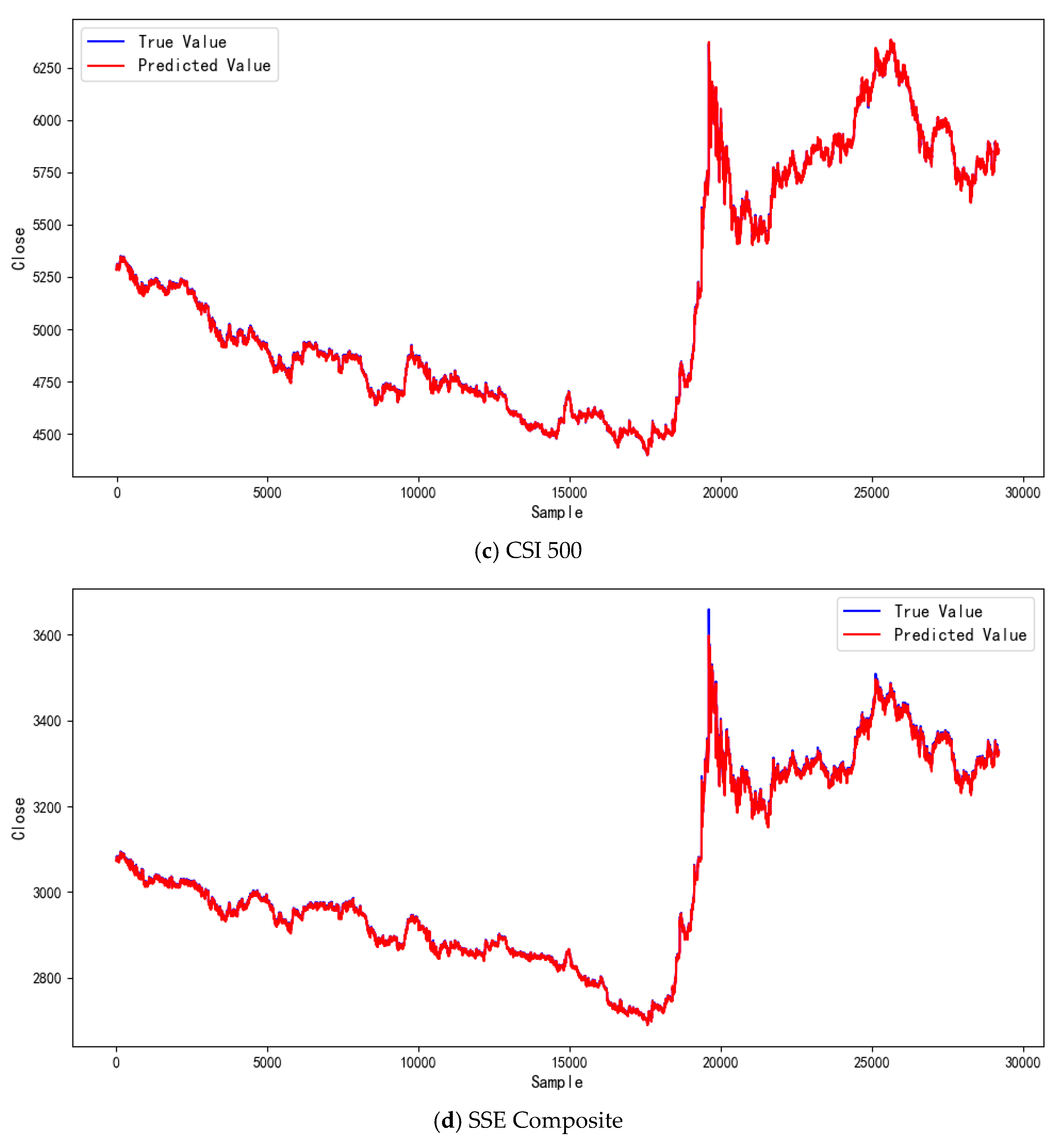
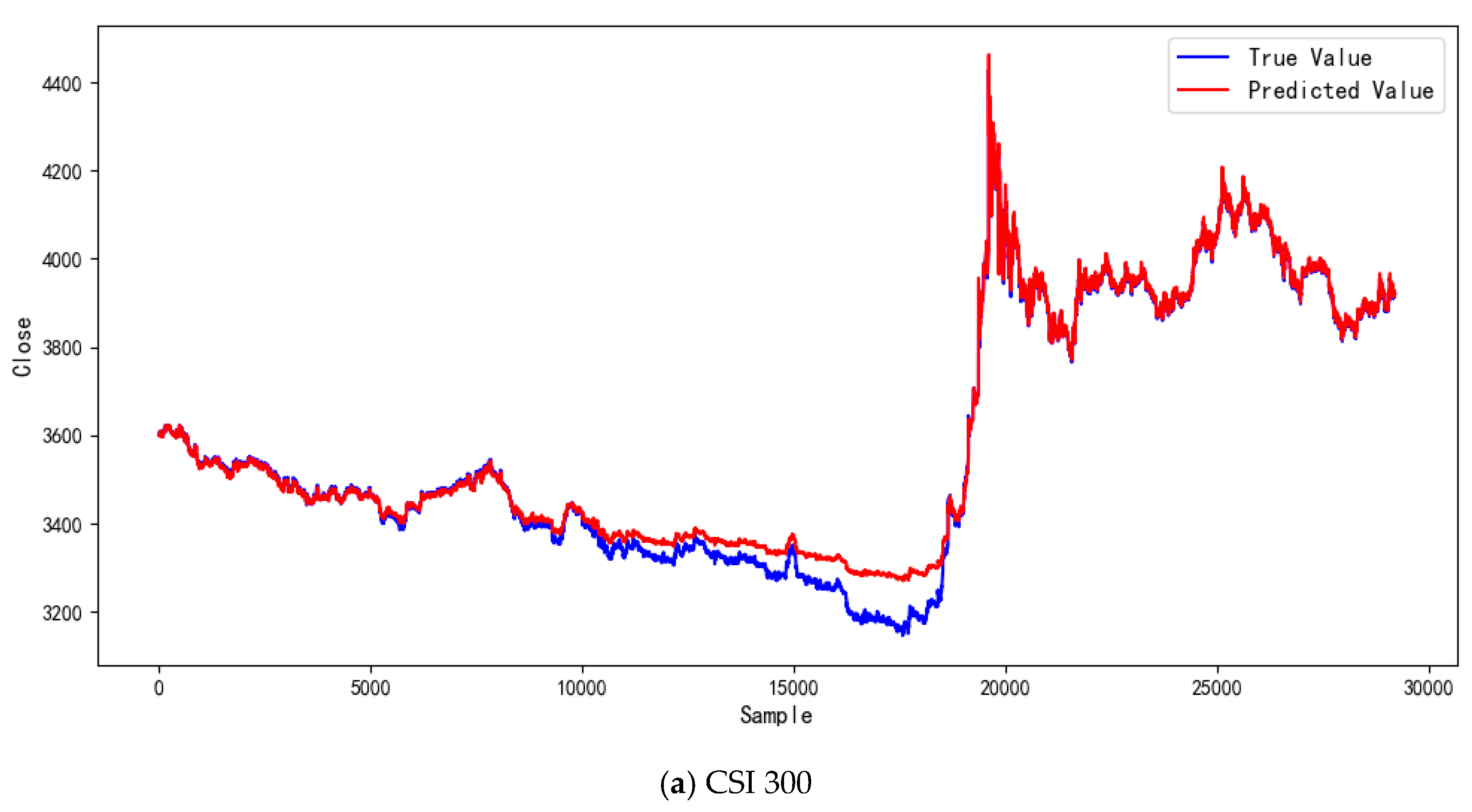
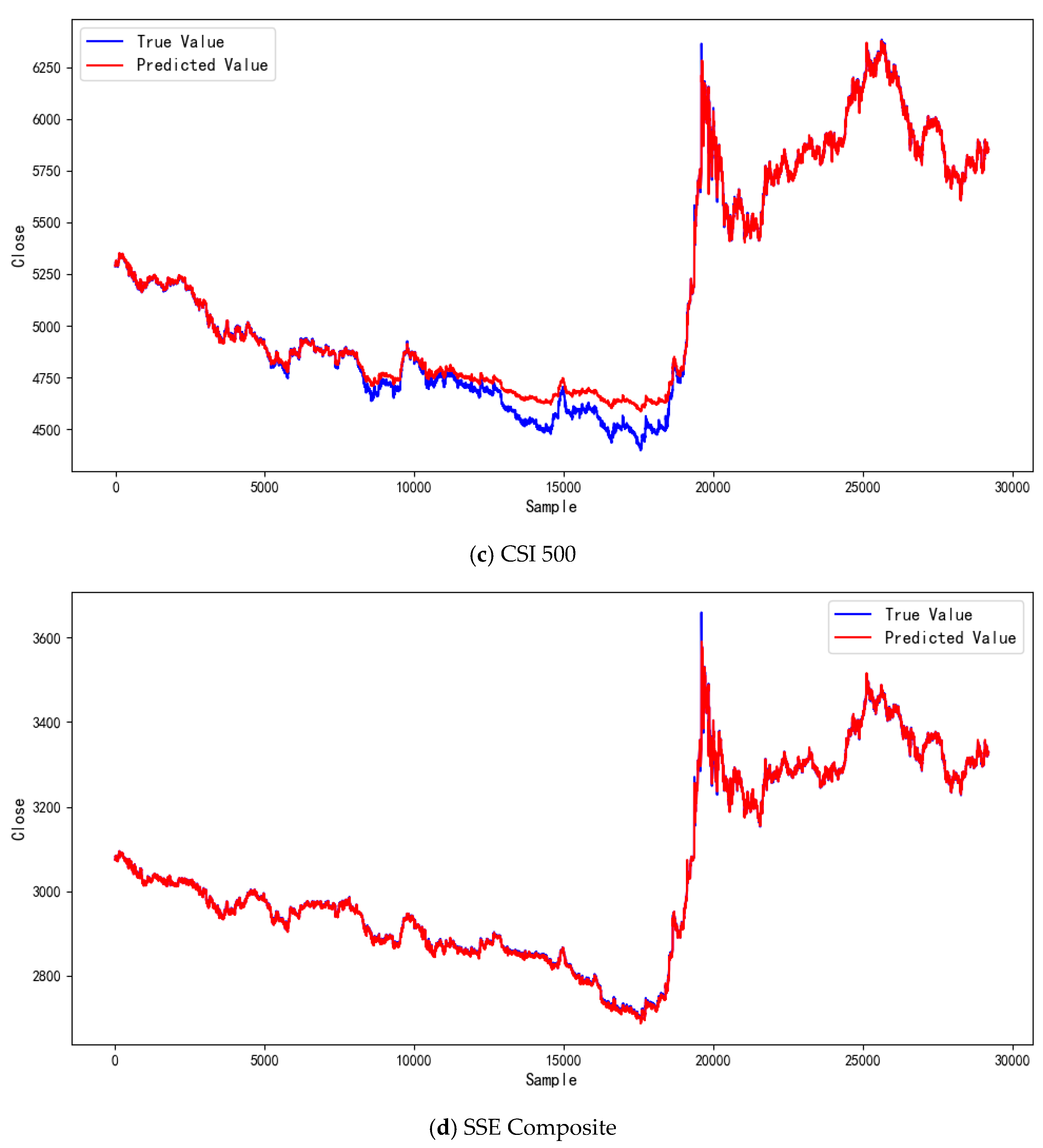
4.3. Comparative Experiments and Result Analysis

To comprehensively evaluate the predictive performance of MSGformer, we conducted comparative experiments against three state-of-the-art deep learning models: Transformer, Pathformer, and Autoformer. The experiments were conducted using four representative Chinese A-share stock indices: CSI 300, SSE 50, CSI 500, and SSE Composite, with 1 min interval trading data collected from January 2019 to December 2024.
Performance was assessed using four standard metrics: R2, MAE, RMSE, and MAPE. These metrics provide a balanced evaluation of model accuracy, error magnitude, and prediction robustness.
As shown in Table 2, MSGformer consistently achieved the lowest MAE, RMSE, and MAPE values across all datasets, while recording the highest R2 scores—indicating excellent fit between predicted and actual values. These results clearly demonstrate the superiority of the hybrid architecture in capturing both short-term volatility and long-term trends in complex financial time series.
As shown in Figure 6, the prediction curve of the MSGformer model (in red) closely overlaps with the actual stock price curve (in blue), particularly in regions characterized by high-frequency fluctuations and trend reversals, where it maintains a high level of fitting accuracy. This result highlights MSGformer’s strong capability in modeling complex nonlinear relationships and long-term dependencies. In contrast, the baseline models shown in Figure 7, Figure 8 and Figure 9 exhibit varying degrees of prediction deviation. Notably, Autoformer demonstrates evident lag and amplified errors on the CSI 500 and SSE Composite indices, indicating insufficient robustness in handling high-frequency volatility.
Moreover, from the plots constructed with “Sample” on the x-axis and “Close” on the y-axis, it is evident that MSGformer not only outperforms other models in trend detection but also demonstrates greater sensitivity to subtle fluctuations. This superior performance is attributed to its integration of the multi-scale graph structure capabilities of MSGNet and the global attention mechanism of Transformer, enabling the model to perceive both local patterns and overall trends simultaneously.
The chart-based analysis further validates the advantages observed in the quantitative evaluation, confirming that MSGformer not only surpasses baseline models in statistical metrics but also achieves better visual fitting and prediction accuracy. This makes it well-suited for high-frequency forecasting tasks in real-world financial markets.
While standard evaluation metrics such as MAE, RMSE, and MAPE were used to quantify prediction accuracy, we acknowledge the importance of further analyzing the structure of forecast errors. In particular, decomposing the mean squared error (MSE) into its bias (mean), variance, and covariance components can provide deeper insight into model behavior. Although such decomposition is not performed in the current study, we consider this a valuable direction for future research to understand the sources of prediction error more granularly.
Upon visual inspection of the prediction curves (Figure 6, Figure 7, Figure 8 and Figure 9), we observed that in certain periods—especially during downward market trends—MSGformer tends to exhibit systematic overestimation errors. This suggests that the model may underperform in capturing abrupt declines or sharp reversals, which are more difficult to predict due to their asymmetrical and volatile nature.
Although the primary analysis focused on comparative performance, we also conducted internal tests (not detailed here) to examine the contribution of MSGformer’s core components. These supplementary ablation experiments support the finding that both the MSGNet module and the Transformer-based self-attention mechanism play essential roles in delivering the model’s high accuracy. This further validates the effectiveness of the hybrid design.
In conclusion, the experimental evidence confirms that MSGformer significantly outperforms baseline models across multiple financial forecasting tasks, delivering robust and accurate predictions even in the face of complex market dynamics.
While this study focuses on representative index time series, we acknowledge that forecasting individual stock prices introduces greater challenges due to increased volatility, noise, and idiosyncratic events (e.g., earnings reports, company-specific news). These factors make generalization more difficult but also represent a more practical application scenario. Although not explored in this study, evaluating MSGformer on individual stocks is a key direction for future work. Such validation will allow us to assess the model’s robustness under lower signal-to-noise conditions and its suitability for finer-grained trading strategies. Stock indices typically exhibit lower volatility and higher signal-to-noise ratios compared to individual securities, which may benefit model stability during training. However, individual stock prices are influenced by more idiosyncratic factors such as company-specific news, liquidity, and investor sentiment. Therefore, verifying the robustness of MSGformer on individual stocks is a necessary next step to assess its generalizability across broader financial scenarios.
In addition to expanding the analysis to individual securities, another important direction for future research involves evaluating the performance of MSGformer across different capital markets. The current study is limited to the Chinese A-share market, which possesses unique structural characteristics such as trading hours, investor composition, and regulatory mechanisms. These factors may affect model behavior and predictive effectiveness. As such, it is important to assess whether MSGformer can generalize to other markets—such as the U.S., European, and emerging markets—where market dynamics and data properties may differ significantly.

5. Conclusions

In this paper, we propose the MSGformer model for financial time series forecasting, specifically tailored to enhance the prediction accuracy of high-frequency stock price movements and market volatility. To evaluate its performance, we conducted extensive experiments using 1 min interval trading data from four representative indices of the Chinese A-share market: the CSI 300, SSE 50, CSI 500, and SSE Composite Indices. The dataset spans from December 2012 to December 2024, covering over a decade of market fluctuations and structural changes. MSGformer was benchmarked against both traditional and state-of-the-art forecasting models.
The experimental results show that MSGformer achieves superior accuracy in both short-term volatility estimation and long-term trend prediction. These findings highlight the model’s practical potential in real-world financial applications, where timely and precise forecasts are essential. Investors leveraging MSGformer’s predictions may obtain improved excess returns and make more informed decisions.
MSGformer’s strength lies in its hybrid architecture, which integrates a multi-scale graph convolutional network (MSGNet) with a Transformer-based self-attention mechanism. This design enables the model to effectively capture complex temporal dependencies and nonlinear patterns inherent in financial time series. Furthermore, the model demonstrates robust and consistent performance across multiple forecasting horizons, including intraday, daily, and weekly intervals.
Quantitative evaluations based on R2, MAE, RMSE, and MAPE indicate that MSGformer consistently outperforms baseline models across various forecasting tasks. It achieves lower prediction errors and higher goodness-of-fit metrics, confirming its effectiveness. Additionally, ablation studies were conducted to assess the contribution of each architectural component. The results confirm that both the MSGNet module and the Transformer-based self-attention mechanism are integral to the model’s performance. Removing either component results in a significant decline in predictive accuracy, thereby validating the benefits of the hybrid design.
Although the current experiments demonstrate the effectiveness of MSGformer on representative Chinese stock indices, future work will investigate its applicability to individual securities. This will enable a more comprehensive assessment of the model’s robustness in high-noise, low-correlation environments, and further validate its practical relevance for fine-grained trading strategies.
Moreover, future work will also explore the application of MSGformer in international markets beyond China. Financial markets differ in volatility regimes, microstructure, and investor behavior across regions. Validating the model on diverse datasets from developed (e.g., S&P 500, DAX) and emerging markets would allow us to assess its robustness, adaptability, and universal applicability, making MSGformer a more globally deployable tool for financial forecasting.
Overall, this study provides valuable insights into the application of deep learning techniques for high-frequency financial forecasting and introduces a robust, interpretable tool for investors and financial decision-makers to manage risk and optimize investment strategies.

Author Contributions

M.Z., conceptualization, methodology, writing—original draft, and supervision; H.Q., writing—original draft and supervision; S.N., formal analysis; Y.L., investigation and data curation. All authors have read and agreed to the published version of the manuscript.

Funding

This research was funded by Key Research Project of Henan Province (231111210500). “Double first-class” discipline creation Project of Surveying and Mapping Science and Technology: GCCYJKT202513.

Data Availability Statement

The original contributions presented in this study are included in the article. Further inquiries can be directed to the corresponding author.

Conflicts of Interest

Author Mingfu Zhu and Shuiping Ni were employed by the company Hebi National Optoelectronic Technology Co, Ltd. The remaining authors declare that the research was conducted in the absence of any commercial or financial relationships that could be construed as a potential conflict of interest.

References

  1. Fama, E.F. Efficient capital markets. J. Financ. 1970, 25, 383–417. [Google Scholar] [CrossRef]
  2. Roll, R. Volatility, correlation, and diversification in a multi-factor world. J. Portf. Manag. 2013, 39, 11–18. [Google Scholar] [CrossRef]
  3. Ongan, S.; Gocer, I. Testing the causalities between economic policy uncertainty and the US stock indices: Applications of linear and nonlinear approaches. Ann. Financ. Econ. 2017, 12, 1750016. [Google Scholar] [CrossRef]
  4. Cortes, C.; Vapnik, V. Support-vector networks. Mach. Learn. 1995, 20, 273–297. [Google Scholar] [CrossRef]
  5. Breiman, L. Random Forests. Mach. Learn. 2001, 45, 5–32. [Google Scholar] [CrossRef]
  6. Cover, T.; Hart, P. Nearest neighbor pattern classification. IEEE Trans. Inf. Theory 1967, 13, 21–27. [Google Scholar] [CrossRef]
  7. Franses, P.H.; Van Dijk, D. Non-Linear Time Series Models in Empirical Finance; Cambridge University Press: Cambridge, UK, 2000. [Google Scholar]
  8. Elizar, E.; Zulkifley, M.A.; Muharar, R.; Zaman, M.H.M.; Mustaza, S.M. A Review on Multiscale-Deep-Learning Applications. Sensors 2022, 22, 7384. [Google Scholar] [CrossRef]
  9. Hochreiter, S.; Schmidhuber, J. Long short-term memory. Neural Comput. 1997, 9, 1735–1780. [Google Scholar] [CrossRef]
  10. LeCun, Y.; Bengio, Y.; Hinton, G. Deep learning. Nature 2015, 521, 436–444. [Google Scholar] [CrossRef]
  11. Bengio, Y.; Simard, P.; Frasconi, P. Learning long-term dependencies with gradient descent is difficult. IEEE Trans. Neural Netw. 1994, 5, 157–166. [Google Scholar] [CrossRef]
  12. Graves, A.; Graves, A. Supervised Sequence Labelling; Springer: Berlin/Heidelberg, Germany, 2012; pp. 5–13. [Google Scholar] [CrossRef]
  13. Vaswani, A.; Shazeer, N.; Parmar, N.; Uszkoreit, J.; Jones, L.; Gomez, A.N.; Kaiser, Ł.; Polosukhin, I. Attention is all you need. In Proceedings of the Advances in Neural Information Processing Systems, Long Beach, CA, USA, 4–9 December 2017; Volume 30. [Google Scholar]
  14. Dosovitskiy, A.; Fischer, P.; Springenberg, J.T.; Riedmiller, M.; Brox, T. Discriminative unsupervised feature learning with convolutional neural networks. In Proceedings of the Advances in Neural Information Processing Systems, Montreal, QC, Canada, 8–13 December 2014; Volume 27. [Google Scholar]
  15. Zhang, L.; Radke, R.J. A Multi-Stream Recurrent Neural Network for Social Role Detection in Multiparty Interactions. IEEE J. Sel. Top. Signal Process. 2020, 14, 554–567. [Google Scholar] [CrossRef]
  16. Keneshloo, Y.; Shi, T.; Ramakrishnan, N.; Reddy, C.K. Deep Reinforcement Learning for Sequence-to-Sequence Models. IEEE Trans. Neural Netw. Learn. Syst. 2019, 31, 2469–2489. [Google Scholar] [CrossRef]
  17. Zeng, A.; Chen, M.; Zhang, L.; Xu, Q. Are Transformers Effective for Time Series Forecasting? Proc. AAAI Conf. Artif. Intell. 2023, 37, 11121–11128. [Google Scholar] [CrossRef]
  18. Nie, Y.; Kong, Y.; Dong, X.; Mulvey, J.M.; Poor, H.V.; Wen, Q.; Zohren, S. A survey of large language models for financial applications: Progress, prospects and challenges. arXiv 2024, arXiv:2406.11903. [Google Scholar] [CrossRef]
  19. Wu, H.; Hu, T.; Liu, Y.; Zhou, H.; Wang, J.; Long, M. Timesnet: Temporal 2d-variation modeling for general time series analysis. arXiv 2022, arXiv:2210.02186. [Google Scholar]
  20. Zhou, T.; Ma, Z.; Wen, Q.; Wang, X.; Sun, L.; Jin, R. Fedformer: Frequency enhanced decomposed transformer for long-term series forecasting. In Proceedings of the International Conference on Machine Learning, Baltimore, MD, USA, 17–23 July 2022; pp. 27268–27286. [Google Scholar] [CrossRef]
  21. Zhou, H.; Zhang, S.; Peng, J.; Zhang, S.; Li, J.; Xiong, H.; Zhang, W. Informer: Beyond Efficient Transformer for Long Sequence Time-Series Forecasting. Proc. AAAI Conf. Artif. Intell. 2021, 35, 11106–11115. [Google Scholar] [CrossRef]
  22. Cheng, W.K.; Bea, K.T.; Leow, S.M.H.; Chan, J.Y.-L.; Hong, Z.-W.; Chen, Y.-L. A Review of Sentiment, Semantic and Event-Extraction-Based Approaches in Stock Forecasting. Mathematics 2022, 10, 2437. [Google Scholar] [CrossRef]
  23. Li, W.; Law, K.L.E. Deep Learning Models for Time Series Forecasting: A Review. IEEE Access 2024, 12, 92306–92327. [Google Scholar] [CrossRef]
  24. Cai, W.; Liang, Y.; Liu, X.; Feng, J.; Wu, Y. MSGNet: Learning Multi-Scale Inter-series Correlations for Multivariate Time Series Forecasting. Proc. AAAI Conf. Artif. Intell. 2024, 38, 11141–11149. [Google Scholar] [CrossRef]
  25. Box, G.E.P.; Jenkins, G.M.; Reinsel, G.C.; Ljung, G.M. Time Series Analysis: Forecasting and Control; John Wiley & Sons: Hoboken, NJ, USA, 2015. [Google Scholar]
  26. Hamilton, J.D. Time Series Analysis; Princeton University Press: Princeton, NJ, USA, 2020. [Google Scholar]
  27. Sims, C.A. Macroeconomics and Reality. Econometrica 1980, 48, 1–48. [Google Scholar] [CrossRef]
  28. Pesaran, M.H.; Shin, Y. An Autoregressive Distributed Lag Modelling Approach to Cointegration Analysis; University of Cambridge: Cambridge, UK, 1995; Volume 9514, pp. 370–413. [Google Scholar]
  29. Engle, R.F. Autoregressive Conditional Heteroscedasticity with Estimates of the Variance of United Kingdom Inflation. Econometrica 1982, 50, 987–1007. [Google Scholar] [CrossRef]
  30. Bollerslev, T. Generalized autoregressive conditional heteroskedasticity. J. Econ. 1986, 31, 307–327. [Google Scholar] [CrossRef]
  31. Ghysels, E.; Santa-Clara, P.; Valkanov, R. Predicting volatility: Getting the most out of return data sampled at different frequencies. J. Econ. 2006, 131, 59–95. [Google Scholar] [CrossRef]
  32. Zhang, G.P. Time series forecasting using a hybrid ARIMA and neural network model. Neurocomputing 2003, 50, 159–175. [Google Scholar] [CrossRef]
  33. Zhang, Y.; Lin, H.; Yang, Z.; Wang, J.; Zhang, S.; Sun, Y.; Yang, L. A hybrid model based on neural networks for biomedical relation extraction. J. Biomed. Inform. 2018, 81, 83–92. [Google Scholar] [CrossRef]
  34. Patel, J.; Shah, S.; Thakkar, P.; Kotecha, K. Predicting stock and stock price index movement using Trend Deterministic Data Preparation and machine learning techniques. Expert Syst. Appl. 2015, 42, 259–268. [Google Scholar] [CrossRef]
  35. Atsalakis, G.S.; Valavanis, K.P. Surveying stock market forecasting techniques—Part II: Soft computing methods. Expert Syst. Appl. 2009, 36, 5932–5941. [Google Scholar] [CrossRef]
  36. Bao, W.; Yue, J.; Rao, Y.; Podobnik, B. A deep learning framework for financial time series using stacked autoencoders and long-short term memory. PLoS ONE 2017, 12, e0180944. [Google Scholar] [CrossRef]
  37. Wang, J.-Z.; Wang, J.-J.; Zhang, Z.-G.; Guo, S.-P. Forecasting stock indices with back propagation neural network. Expert Syst. Appl. 2011, 38, 14346–14355. [Google Scholar] [CrossRef]
  38. Nti, I.K.; Adekoya, A.F.; Weyori, B.A. Efficient Stock-Market Prediction Using Ensemble Support Vector Machine. Open Comput. Sci. 2020, 10, 153–163. [Google Scholar] [CrossRef]
  39. Tsantekidis, A.; Passalis, N.; Tefas, A.; Kanniainen, J.; Gabbouj, M.; Iosifidis, A. Forecasting Stock Prices from the Limit Order Book Using Convolutional Neural Networks. In Proceedings of the 2017 IEEE 19th Conference on Business Informatics (CBI), Thessaloniki, Greece, 24–27 July 2017; Volume 1, pp. 7–12. [Google Scholar] [CrossRef]
  40. Sezer, O.B.; Gudelek, M.U.; Ozbayoglu, A.M. Financial time series forecasting with deep learning: A systematic literature review: 2005–2019. Appl. Soft Comput. 2020, 90, 106181. [Google Scholar] [CrossRef]
  41. Fischer, T.; Krauss, C. Deep learning with long short-term memory networks for financial market predictions. Eur. J. Oper. Res. 2018, 270, 654–669. [Google Scholar] [CrossRef]
  42. Chen, K.; Zhou, Y.; Dai, F. A LSTM-based method for stock returns prediction: A case study of China stock market. In Proceedings of the IEEE International Conference on Big Data (Big Data), Santa Clara, CA, USA, 29 October–1 November 2015; pp. 2823–2824. [Google Scholar]
  43. Chong, E.; Han, C.; Park, F.C. Deep learning networks for stock market analysis and prediction: Methodology, data representations, and case studies. Expert Syst. Appl. 2017, 83, 187–205. [Google Scholar] [CrossRef]
  44. Nelson, D.M.Q.; Pereira, A.C.M.; de Oliveira, R.A. Stock market’s price movement prediction with LSTM neural networks. In Proceedings of the 2017 International Joint Conference on Neural Networks (IJCNN), Anchorage, AK, USA, 14–19 May 2017; pp. 1419–1426. [Google Scholar]
  45. Wan, A.; Chang, Q.; Al-Bukhaiti, K.; He, J. Short-term power load forecasting for combined heat and power using CNN-LSTM enhanced by attention mechanism. Energy 2023, 282, 128274. [Google Scholar] [CrossRef]
  46. Wu, H.; Xu, J.; Wang, J.; Long, M. Autoformer: Decomposition transformers with auto-correlation for long-term series forecasting. Adv. Neural Inf. Process. Syst. 2021, 34, 22419–22430. [Google Scholar] [CrossRef]
  47. Huang, X.; Tang, J.; Shen, Y. Long time series of ocean wave prediction based on PatchTST model. Ocean Eng. 2024, 301, 117572. [Google Scholar] [CrossRef]
  48. Woo, G.; Liu, C.; Sahoo, D.; Kumar, A.; Hoi, S. Etsformer: Exponential smoothing transformers for time-series forecasting. arXiv 2022, arXiv:2202.01381. [Google Scholar] [CrossRef]
Figure 2. The Transformer model architecture.
Electronics 14 02457 g002
Figure 3. The structure of the self-attention mechanism.
Electronics 14 02457 g003
Figure 4. The framework of MSGformer.
Electronics 14 02457 g004
Figure 5. Moving window methods: Features and labels are constructed from the observed time series using the moving window method. In each prediction, data labeled in blue are used as input features to the model, while the next data labeled in green are used as output labels.
Electronics 14 02457 g005
Figure 6. The prediction curve generated by the MSGformer model is presented below. In this figure, the blue line denotes the actual stock index price.
Electronics 14 02457 g006aElectronics 14 02457 g006b
Figure 7. The prediction curve generated by the Transformer model is presented below. In this figure, the blue line denotes the actual stock index price.
Electronics 14 02457 g007aElectronics 14 02457 g007b
Figure 8. The prediction curve generated by the Pathformer model is presented below. In this figure, the blue line denotes the actual stock index price.
Electronics 14 02457 g008aElectronics 14 02457 g008b
Figure 9. The prediction curve generated by the Autoformer model is presented below. In this figure, the blue line denotes the actual stock index price.
Electronics 14 02457 g009aElectronics 14 02457 g009b
Table 1. Experimental environment.
Configuration
CPUIntel Core i7-10700K (Intel Corp., Santa Clara, CA, USA)
GPUNVIDIA GeForce RTX 4060 Ti (NVIDIA Corp., Santa Clara, CA, USA)
CUDACUDA 12.4 (NVIDIA Corp., Santa Clara, CA, USA)
Python versionPython 3.9 (Python Software Foundation, Wilmington, DE, USA)
Memory32 GB RAM
SystemWindows (Microsoft Corp., Redmond, WA, USA)
Table 2. Results of ten independent experiments on four datasets using three evaluation metrics (R2, MAE, RMSE, and MAPE).
IndexModels R 2 MAERMSEMAPE
CSI 300Transformer0.990510.817913.34150.0038
Pathformer0.989411.387512.92320.0031
Autoformer0.984913.204217.06850.0061
MSGformer0.994110.228212.65220.0024
SSE 50Transformer0.99859.22209.88910.0021
Pathformer0.99819.41568.34230.0026
Autoformer0.99828.15907.88910.0025
MSGformer0.99877.85766.82960.0016
CSI 500Transformer0.984411.895411.77710.0035
Pathformer0.99518.36489.56040.0047
Autoformer0.983615.637113.89850.0054
MSGformer0.99716.45207.56040.0018
SSE CompositeTransformer0.99132.56854.17780.0013
Pathformer0.99542.50813.97780.0009
Autoformer0.99242. 96874.93670.0011
MSGformer0.99962.25533.92670.0007
Disclaimer/Publisher’s Note: The statements, opinions and data contained in all publications are solely those of the individual author(s) and contributor(s) and not of MDPI and/or the editor(s). MDPI and/or the editor(s) disclaim responsibility for any injury to people or property resulting from any ideas, methods, instructions or products referred to in the content.

