Broadband Measurement Algorithm Based on Smooth Linear Segmented Threshold Wavelet Denoising and Improved VMD-Prony

Abstract

Accurate measurement of broadband signals is fundamental to the broadband oscillation analysis of power grids. However, the measurement process of broadband signals generally suffers from noise interference and insufficient measurement accuracy. To address these issues, this study introduces a novel broadband measurement algorithm that integrates smooth linear segmented threshold (SLST) wavelet denoising with a fusion of the improved variational mode decomposition (VMD) and Prony methods. Initially, noise reduction preprocessing is designed for broadband signals based on the smooth linear segmented threshold wavelet denoising method to reduce the interference of noise on the measurement process, and two evaluation indices are established based on Pearson’s correlation coefficient and the signal-to-noise ratio (SNR) to assess the effectiveness of noise reduction. Subsequently, mutual information entropy and energy entropy are employed to optimize the parameters of VMD to enhance measurement precision. The denoised signal is decomposed into several modes with distinct center frequencies using the parameter-optimized VMD, thereby simplifying the signal processing complexity. Concurrently, the Prony algorithm is integrated to accurately identify the parameters of each mode, extracting frequency, amplitude, and phase information to achieve precise broadband signal measurement. The simulation results confirm that the proposed algorithm effectively reduces noise interference and enhances the measurement accuracy of broadband signals.

1. Introduction

The integration of numerous power electronic devices due to high renewable energy penetration has altered power system dynamics, leading to frequent broadband oscillation events [1,2,3]. Unlike traditional power system oscillations, these span from a few Hertz to kilohertz with significant noise interference, which seriously threatens the safe and stable operation of the power system [4,5].

Broadband oscillation events have occurred frequently and have had a wide range of impacts. In 2015, sub-synchronous and super-synchronous oscillations occurred at a wind farm in Xinjiang China, with the presence of 27–33 Hz and its complementary frequency 67–73 Hz component in the current, resulting in the shutdown of a thermal power unit 300 km away [6,7]. In 2017, three sub-synchronous oscillations with frequencies between 20 and 30 Hz occurred in Texas, USA, causing wind turbine trips and series capacitor bypasses [8]. In 2019, a sub-synchronous oscillation at a wind farm in the London area of the United Kingdom caused 300 turbines to go off grid and left 1.1 million residents without power [9]. The above broadband oscillation events severely impact the safe and stable operation of the power system; thus, research into the accurate measurement of broadband signals is imperative. However, in the actual measurement process, the signals are often compromised by various noises, introducing significant errors to the measurement results. Therefore, how to effectively reduce noise and accurately measure the broadband oscillation signal has become an urgent problem to be solved.

Common noise reduction methods for broadband signals in power systems include adaptive filters, compressed sensing, and wavelet transform. Adaptive filters adjust parameters based on signal autocorrelation, suitable for unknown signal and noise characteristics, but they are computationally complex and sensitive to initial parameter settings [10]. Compressed sensing recovers sparse signals from limited measurements, ideal for high-dimensional data, but requires prior knowledge of signal sparsity and involves high computational complexity [11,12]. Wavelet transform (WT) offers multi-scale analysis, effectively capturing local signal features, analyzing different frequency ranges, and removing noise with low computational complexity and ease of implementation [13,14], the empirical wavelet transform (EWT) is an important improvement method to the wavelet transform, which is able to adaptively construct a wavelet filter bank according to the spectral characteristics of the signal, and shows better noise separation ability in non-smooth signal processing, but the computational complexity is high [15].

Common broadband measurement algorithms in power systems can be divided into three categories: Fast Fourier Transform (FFT), modern spectral estimation methods and mode decomposition algorithms. FFT, a simple frequency-domain method, is widely used but limited by resolution tied to window length, spectral leakage, and fence effects [16,17,18]. Modern spectral methods, including Prony, ESPRIT, and MUSIC, offer high-resolution measurement of harmonics and inter-harmonics, directly calculating amplitude, phase, and frequency. However, Prony is noise sensitive at low SNR [19,20], ESPRIT struggles in high-noise environments [21], and MUSIC, despite a high-frequency resolution, has reduced performance and a high computational load at low SNRs [22]. Mode decomposition methods, such as EMD, LMD, ICEEMDAN, FMD and REMD, decompose signals into smoother sub-signals to reduce interference. EMD and LMD are noise sensitive and prone to mode aliasing and endpoint effects [23,24,25], while ICEEMDAN significantly reduces modal aliasing through adaptive noise addition and multiple ensemble averaging, but increases computational complexity [26]. FMD utilizes an adaptive FIR filter to achieve accurate signal decomposition, but its application is limited primarily to mechanical fault signals [27,28]. RLMD mitigates endpoint effects through mirror extension algorithms, enhancing decomposition accuracy, but remains sensitive to noise [29]. Compared to other methods, VMD reduces modal aliasing and endpoint effects through optimized parameter selection, improving decomposition accuracy [30]. Furthermore, VMD can be optimized by adjusting its parameters, allowing for mode decomposition tailored to the characteristics of various signals [31]. However, VMD alone cannot fully characterize each of IMF’s parameters, leaving limitations in parameter identification [32].

In recent years, researchers have proposed some improved broadband measurement algorithms that are optimized based on traditional methods. The literature [33] introduced a fast Taylor–Fourier transform (FTFT) algorithm, using Taylor series for dynamic signal tracking in broadband monitoring. The literature [34] developed an adaptive accelerated MUSIC algorithm, improving frequency scanning speed and robustness under noise for transient power system conditions. The literature [35] uses Wavelet Packet Transform (WPT) preprocessing to suppress the noise, combined with ICEEMDAN to extract the effective IMF components, and finally resolves the signal parameters by Hilbert Transform (HT). The literature [36] proposed an EMD-assisted Prony algorithm, which integrates EMD’s signal decomposition capability with Hurst index-based noise identification to effectively eliminate noise. The denoised signals are then processed using Prony for parameter identification, enabling high-precision measurement and analysis of power system signals.

The general idea of this paper has similarities with the literature [36]; both adopt the idea of combining mode decomposition and Prony algorithm, but there are significant differences in the technical implementation. This study innovatively adopts a three-stage cascade processing architecture: firstly, an improved smoothed linear segmented threshold wavelet denoising method is proposed, and through the dynamic threshold adjustment mechanism and transition region smoothing processing, the high-frequency weak component of the signal is retained in its entirety while effectively suppressing the noise, and the high-quality input signal is provided for the subsequent measurement of broadband signals. A dual optimization based on information entropy and energy entropy is then introduced on the basis of the traditional VMD to realize the modal number and penalty factor optimization. Then, a dual optimization strategy based on information entropy and energy entropy is introduced on the basis of the traditional VMD to realize the adaptive matching of modal number and penalty factor, which ensures that the decomposed modal components have clear physical meanings and good separation characteristics in the frequency domain, so as to avoid the common modal aliasing problem. Finally, the Prony algorithm is applied to the optimized modal components. Since each modal component has been pre-processed and optimized for the decomposition and has a relatively simple frequency component, the Prony only needs to process the low-order model to realize high-precision parameter identification.

In summary, this paper proposes a broadband measurement algorithm based on smooth linear segmented threshold wavelet noise reduction and improved VMD-Prony, aiming at solving the problems of noise interference and insufficient measurement accuracy during the measurement of broadband signals. The main contributions of this paper are as follows:

(1)

A smooth linear segmented threshold (SLST) wavelet denoising method is proposed. By setting upper and lower thresholds and smoothing the coefficients within the threshold range, the method effectively reduces noise interference while retaining the effective information of the signal and improving signal quality.

(2)

The VMD algorithm is improved to optimize the number of modes and the penalty factor. By selecting the number of modes with the largest mutual information entropy, the over-decomposition and under-decomposition phenomena are avoided, and the accuracy of the decomposition results is guaranteed; by minimizing the energy entropy and selecting the optimal penalty factor, the energy distribution of each mode in the frequency domain is concentrated as much as possible, which improves the accuracy of the signal decomposition, and avoids the phenomenon of modal overlapping effectively.

(3)

The Prony is applied to each modal function after VMD decomposition, which realizes the accurate identification of parameter information, such as frequency, amplitude and phase of each mode, thus realizing the accurate measurement of broadband signals.

The rest of the paper is organized as follows. Section 2 describes the overall design framework of the broadband measurement algorithm. Section 3 details the principle and improvement part of the algorithm. Section 4 performs the validation using the proposed algorithm. Section 5 discusses the proposed algorithm. Section 6 summarizes the paper.

2. Overall Design of Broadband Measurement Algorithms

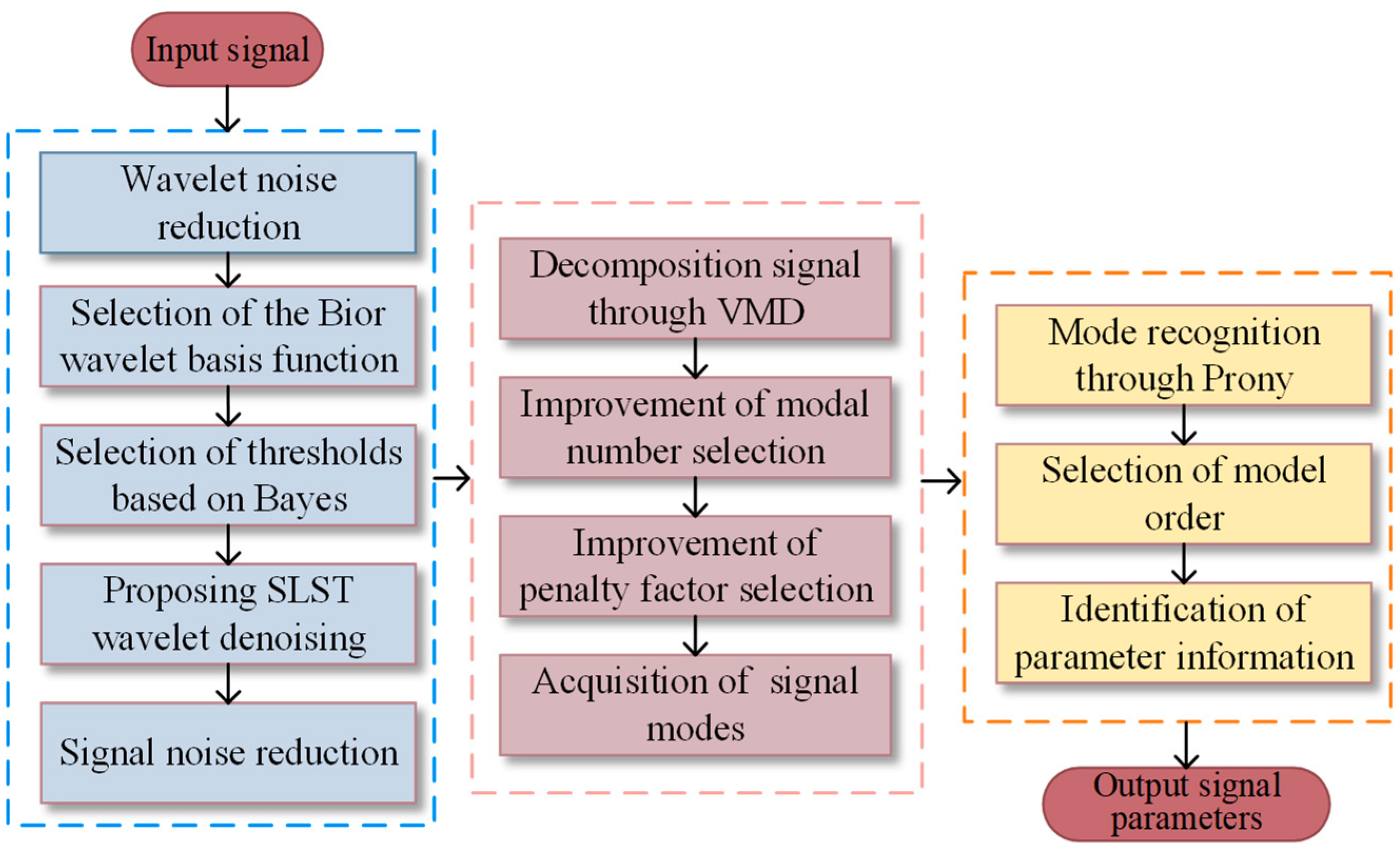
To address the issues of noise interference and the lack of accuracy in signal recognition during the measurement of broadband signals, this paper proposes a novel broadband measurement algorithm that integrates smooth linear segmented threshold wavelet denoising with an improved VMD-Prony. The overall design block diagram of the proposed algorithm is depicted in Figure 1.

The main steps include:

Step 1: Signal Denoising. The broadband signal is subjected to multi-scale wavelet decomposition to yield a set of wavelet coefficients. An appropriate threshold is selected for these coefficients, followed by wavelet inverse transformation of the threshold coefficients to complete the denoising process. Additionally, the effectiveness of the noise reduction is evaluated by Pearson’s correlation coefficient and SNR.

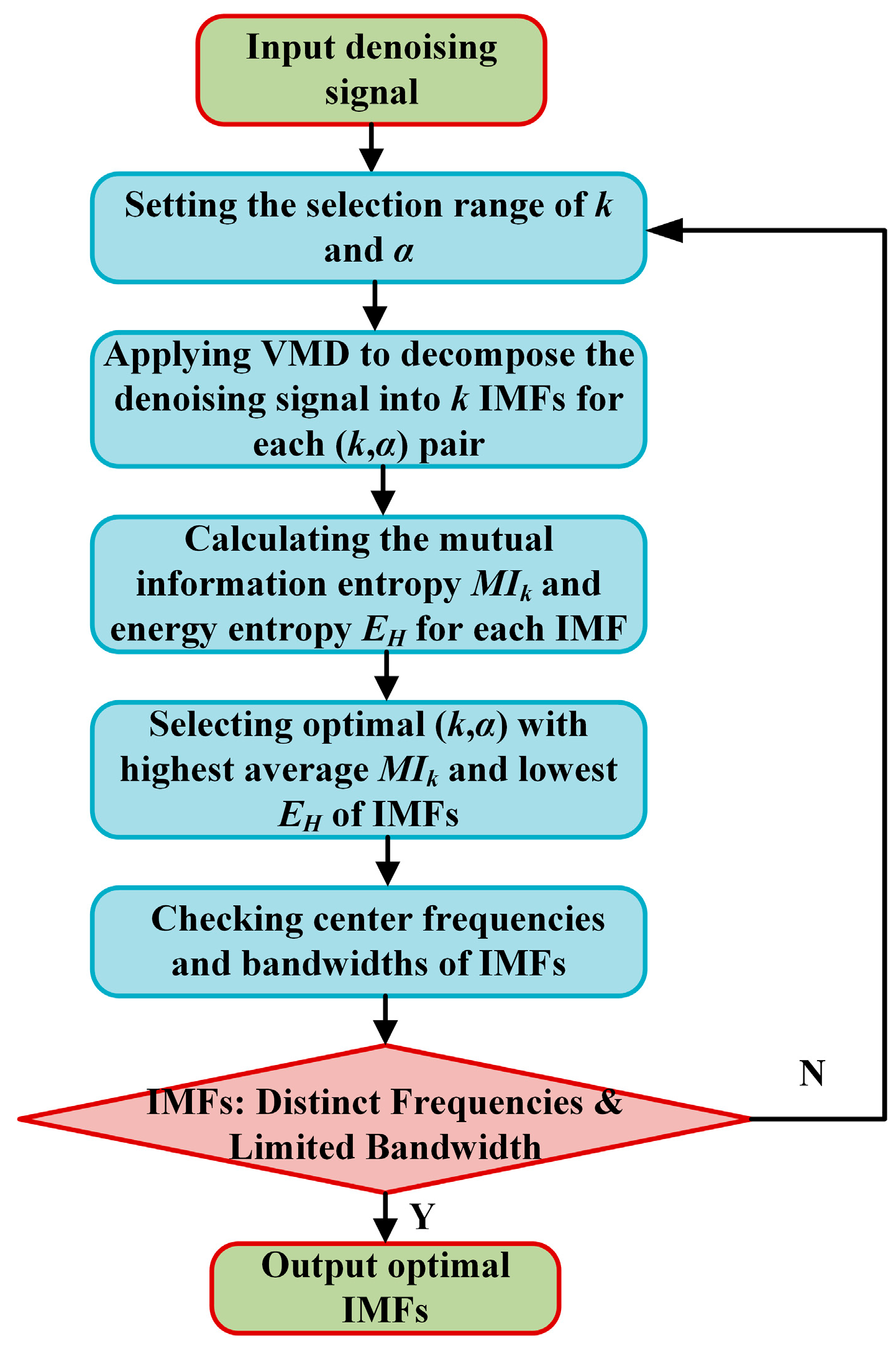
Step 2: Mode Decomposition. To address the presence of multiple signal components at varying frequencies within the broadband signal, the VMD algorithm is employed to decompose the signal into several distinct modes, each characterized by a finite bandwidth and a central frequency. The number of modes k and the penalty factor α are optimized based on mutual information entropy and energy entropy criteria, ensuring that the reconstructed signal from the sum of modes closely matches the original broadband signal, while minimizing the total bandwidth across all modes.

Step 3: Parameter Identification. For each decomposed mode, the Prony is employed to identify the parameters. The model order p is selected based on the characteristics of the individual modes. Prony equations are constructed using the data points of each mode. The parameters, including frequency, amplitude, and phase of the signals, are determined by solving the resulting system of equations. Subsequently, the signals are reconstructed using the identified parameter information.

3. Principles and Methods

3.1. Wavelet Denoising and Its Improvement

Wavelet denoising decomposes a signal into multiple frequency scales using wavelet transform, applies thresholding to remove noise, and reconstructs the denoised signal [13,14]. Common wavelet basis functions include Daubechies, Symlet, and Biorthogonal [37,38], with threshold selection methods, such as Bayes Shrink, False Discovery Rate (FDR), and Stein’s Unbiased Risk Estimate (SURE) Shrinkage, determining denoising effectiveness. Improper thresholds may either filter out useful signal components or retain excessive noise, impacting subsequent analysis.

For the actual noise-containing situation of broadband oscillation signal, this paper selects Biorthogonal wavelet as the wavelet basis function and selects the threshold value according to Bayes. The calculation formula is as follows:

$${\lambda }_j={\displaystyle \frac{{\sigma }^2}{{\sigma }_j^2}}$$

(1)

In (1), λ_j is the determined threshold, and σ and σ_j are the standard deviation of the noise and wavelet coefficients, respectively, which can be calculated by (2) and (3) as follows:

$$\sigma ={\displaystyle \frac{\mathrm{median}(|d_j|)}{0.6745}}$$

(2)

$$(2{\sigma }_j^2={\displaystyle \frac{1}{N_j}}\sum _{i=1}^{N_j}{d}_{j,i}^2)$$

(3)

where d is the wavelet coefficients obtained by wavelet transform of the original signal; N is the total number of wavelet coefficients; j is the number of wavelet decomposition layers; and i is the sampling point.

Wavelet coefficients are processed using thresholding techniques, such as Hard Thresholding (HT), Soft Thresholding (ST), Median Thresholding, and Mean Thresholding, with HT and ST being most common in engineering applications. HT sets coefficients below the threshold to zero, preserving signal characteristics but causing discontinuities. ST subtracts the threshold from coefficients above zero, yielding smoother signals but potentially losing detail. The principles of HT and ST can be expressed by (4) and (5):

$${\stackrel{\wedge }{d}}_{j,i}=\left\{\begin{array}{cc}{d}_{j,i}& \left|d_{j,i}\right|\ge {\lambda }_j\\ 0& \left|d_{j,i}\right|<{\lambda }_j\end{array}\right.$$

(4)

$${\stackrel{\wedge }{d}}_{j,i}=\mathrm{sign}(d_{j,i})\cdot \max (|d_{j,i}|-{\lambda }_j,0)$$

(5)

To overcome these limitations, this paper proposes a smooth linear segmented threshold (SLST) method, using adaptive upper and lower thresholds with a smoothing factor, as shown in Equation (6):

$${\stackrel{\wedge }{d}}_j=\left\{\begin{array}{ll}{d}_j\hfill & \left|d_j\right|>{\lambda }_2\hfill \\ d_j\cdot \mu ,\hfill & {\lambda }_1\le \left|d_j\right|\le {\lambda }_2\hfill \\ 0\hfill & \left|d_j\right|<{\lambda }_1\hfill \end{array}\right.$$

(6)

where μ is the reduction factor, λ₁ is the lower threshold, determined according to the Bayes method of Equation (1), λ₂ is the upper threshold, and λ₂ is set to be 1.5λ₁ based on the theoretical needs of the smoothing threshold design to ensure that the width of the transition region is sufficient to smooth the wavelet coefficients and, at the same time, to avoid excessive attenuation of the signal.

The reduction factor can be calculated by (7):

$$\mu =\left(1-{\displaystyle \frac{{\lambda }_1^2}{d_j^2+{\lambda }_1^2}}\right)$$

(7)

The SLST wavelet denoising method introduces adaptive upper and lower thresholds for processing wavelet coefficients. Coefficients below the lower threshold are set to zero to eliminate noise, while those above the upper threshold remain unchanged to preserve key signal features. For coefficients between thresholds, a reduction factor, derived from noise and coefficient standard deviations, is applied to smooth the signal.

When d_j is small, the reduction factor approaches zero, leading to a significant decrease in the wavelet coefficient and ensuring a smooth signal transition. Conversely, when d_j is large, the reduction factor tends towards one, causing the wavelet coefficients to remain largely unchanged, thereby reducing the loss of high-frequency components to some extent. Unlike traditional hard or soft thresholding, SLST achieves superior noise suppression and signal fidelity through multi-scale adaptive thresholding, enhancing broadband signal quality for subsequent VMD.

3.2. Variational Mode Decomposition and Its Improvement

3.2.1. VMD Fundamentals

Variational Mode Decomposition (VMD) extracts intrinsic modal functions (lMFs) by solving a constrained variational optimization problem. Assuming that the signal can be decomposed into k modes by VMD, and each mode is a finite bandwidth with a center frequency ω_k, the variational problem can be described as finding k modal functions u_k(t), where the sum of each mode is equal to the input signal x(t) and the sum of the bandwidths of each mode is minimized.

The variational problem is formulated as

$$\left\{\begin{array}{l}{\min }_{\left\{u_k\right\},\left\{{\omega }_k\right\}}\left\{{\displaystyle \sum _{k=1}^K{‖{\partial }_t\left[\left(\delta \left(t\right)+\frac{j}{\pi t}\right)\times u_k\left(t\right)\right]\times e^{-j{\omega }_{k}t}‖}_2^2}\right\}\\ s.t.{\displaystyle \sum _{k=1}^K{u}_k}\left(t\right)=x\left(t\right)\end{array}\right.$$

(8)

where ∂_t denotes the time derivative, δ(t) is the impulse function and j denotes the imaginary part. The Lagrange operator λ(t) is introduced with penalty factor α to transform the constrained problem into the corresponding unconstrained problem by (9):

$$\begin{array}{l}L\left(\left\{u_k\right\},\left\{{\omega }_k\right\},\lambda \right)=\alpha {\displaystyle \sum _{k=1}^K{‖{\partial }_t\left[\left(\delta \left(t\right)+\frac{j}{\pi t}\right)\times u_k\left(t\right)\right]\times e^{-j{\omega }_{k}t}‖}_2^2}\\ +{‖f\left(t\right)-{\displaystyle \sum _{k=1}^K{u}_k}\left(t\right)‖}_2^2+〈\lambda \left(t\right),f\left(t\right)-{\displaystyle \sum _{k=1}^K{u}_k}\left(t\right)〉\end{array}$$

(9)

A further solution is carried out by Alternate Direction Method of Multipliers (ADMM), where the modal function u_k(t), the center frequency ω_k and the Lagrange multiplier λ are continuously updated iteratively, as shown in (10)–(12):

$${\widehat{u}}_k^{n+1}\left(\omega \right)={\displaystyle \frac{\widehat{f}\left(\omega \right)-{\displaystyle \sum _{i\ne k}{\widehat{u}}_i}\left(\omega \right)+\frac{\widehat{\lambda }\left(\omega \right)}{2}}{1+2\alpha {\left(\omega -{\omega }_k\right)}^2}}$$

(10)

$${\omega }_k^{n+1}={\displaystyle \frac{{\displaystyle {\int }_0^{\infty }\omega }{\left|{\widehat{u}}_k\left(\omega \right)\right|}^{2}d\omega }{{\displaystyle {\int }_0^{\infty }{\left|{\widehat{u}}_k\left(\omega \right)\right|}^2}d\omega }}$$

(11)

$${\widehat{\lambda }}^{n+1}\left(\begin{array}{c}\omega \end{array}\right)={\widehat{\lambda }}^n\left(\begin{array}{c}\omega \end{array}\right)+\gamma \left[\widehat{f}\left(\begin{array}{c}\omega \end{array}\right)-{\displaystyle \sum _{k=1}^K{\widehat{u}}_k^{n+1}}\left(\begin{array}{c}\omega \end{array}\right)\right]$$

(12)

where n denotes the iteration index and γ denotes the noise tolerance parameter.

3.2.2. Improvement of Modal Number Selection Method

The value of the modal number k in the VMD determines the accuracy of the final decomposition result. If the value of k is too small, it will lead to incomplete mode decomposition; if the value of k is too large, the over-decomposition phenomenon will occur.

This study introduces a method to determine the optimal k using a correlation coefficient derived from mutual information entropy, which measures the interdependence between a decomposed mode and the original signal. Modes with high entropy capture significant signal information, indicating their validity, while low-entropy modes suggest virtual artifacts from over-decomposition. The steps for designing the modal number by mutual information entropy are as follows:

Step 1: Perform VMD decomposition of the original signal x to obtain k modes.

Step 2: Calculate the entropy of the original signal; the entropy H(x) is given by (13):

$$H(x)=-{\displaystyle \sum _{i}p}(x_i){\log }_{2}p(x_i)$$

(13)

where p(x_i) is the probability distribution of the ith value in the original signal x.

Step 3: For each mode, calculate the conditional entropy, which is given by (14):

$$H(x|x_k)=-{\displaystyle \sum _{i,j}p}(x_i,x_{k,j}){\log }_2{\displaystyle \frac{p(x_i,x_{k,j})}{p(x_{k,j})}}$$

(14)

where x_i is the ith mode, x_k is the kth mode, p(x_k,j) is the probability distribution of the jth frequency component of x_k, and p(x_i,x_k,j) is the joint probability distribution of the jth frequency components of x_i and x_k.

Step 4: For each modality, calculate the mutual information entropy; the mutual information entropy MI_k is given by (15):

$$M{I}_k={\displaystyle \frac{H(x)-H(x|x_k)}{H(x)}}$$

(15)

Step 5: The value corresponding to the maximum mutual information entropy is chosen as the optimal modal number, and (16) for choosing the optimal modal number k_opt:

$$k_{opt}=\arg {\max }_{k}M{I}_k$$

(16)

The mutual information entropy increases and then decreases as the value of k increases. When this entropy starts to decrease, it indicates that over decomposition occurs, the increased number of modes does not lead to more effective information, but instead, it may introduce redundant information, leading to a decrease in the overall information retention. Therefore, choosing the value of k corresponding to the maximum mutual information entropy as the optimal number of modes k_opt, strikes a balance between the completeness of the signal decomposition and the avoidance of redundant modes.

3.2.3. Improvement of Penalty Factor Selection Method

In VMD, the penalty factor α significantly influences the bandwidth of decomposed modes by controlling their deviation from the center frequency in the frequency domain. A larger α reduces mode bandwidth, minimizing deviation and enhancing mode concentration, which mitigates modal aliasing and improves feature extraction accuracy. Conversely, a smaller α increases bandwidth, potentially incorporating multiple frequency components and dispersing modes.

In this paper, the penalty factor α is designed by introducing energy entropy. Energy entropy provides a quantitative index to quantify the concentration of modes in the frequency domain by using the distribution of the energy of each mode, to indirectly affect the modal bandwidth and guide the selection of the penalty factor.

By minimizing the energy entropy, the optimal penalty factor is found, so that the energy distribution of the modes is concentrated as much as possible, and the sum of the bandwidths of the modes is minimized. The energy entropy design penalty factor α step is as follows:

Step 1: VMD decomposition of the original signal x is performed to obtain k modes.

Step 2: The VMD decomposition yields k modes, and for each mode the energy is calculated by (17):

$$E_k={\displaystyle \int |}{u}_k(\omega ){|}^{2}d\omega$$

(17)

Step 3: Calculate the energy entropy of each modal energy. The energy entropy E_H is used to quantify the concentration of modes in the frequency domain as follows:

$$EH=-{\displaystyle \sum _{i=1}^{N}pi}{\log }_2(p_i)$$

(18)

where p_i is the ratio of the energy of the ith frequency component to the total energy and N is the total number of frequency components in the mode.

Step 4: For each value of the penalty factor α, Step 2 and Step 3 are repeated, and the corresponding energy entropy E_H is computed. The penalty factor is selected through (19) to minimize the energy entropy as follows:

$${\alpha }_{\mathrm{opt}}=\arg {\min }_{\alpha }{\displaystyle \sum _{k=1}^{K}E}H$$

(19)

3.2.4. Joint Optimization of Modal Numbers and Penalty Factors

Although the selection methods for the modal number k and the penalty factor α have been improved by mutual information entropy and energy entropy, respectively, their optimization is a coupled process in practice because these two parameters together determine the quality of the IMFs obtained from the decomposition.

The specific procedure is as follows: initially, we define the selection range for the modal number k and penalty factor α (where k ∈ [2, 15], α ∈ [500, 5000]). For each pair (k, α), the VMD algorithm is applied to decompose the denoised signal into k IMFs. Subsequently, two metrics—the mutual information entropy MI_k and the energy entropy E_H—are computed. Here, MI_k is used to evaluate the amount of information captured by the IMFs, and E_H is used to evaluate the concentration of the energy distribution of each IMF in the frequency domain. By maximizing the average MI_k of all IMFs and minimizing the E_H, thereby ensuring the effectiveness of signal decomposition and minimizing modal aliasing. Next, a validation step is conducted by examining the center frequency and bandwidth of the IMFs. If the center frequencies of the IMFs are unclear or the bandwidths are excessively large, the ranges of k and α are adjusted, and the process is repeated. Figure 2 presents the flowchart of the joint optimization of modal number and penalty factor in VMD.

3.3. Prony Algorithm

3.3.1. Prony Fundamentals

Prony fits the sampled data at equal time intervals with a linear combination of complex exponential terms. Assuming that the sampled data is x(n), the estimates of the inputs x(0), x(1), …, x(N − 1) can be expressed as (20):

$$\stackrel{\wedge }{x}(n)={\displaystyle \sum _{i=1}^p{b}_i}{z}_i\hspace{1em}n=0,1,\dots ,N-1$$

(20)

where p is the order of the model, N is the number of sampled data points, and b_i and z_i are both complex numbers.

$$b_i=A_i{\mathrm{e}}^{(\mathrm{j}{\theta }_i)}$$

(21)

$$z_i={\mathrm{e}}^{({\alpha }_i+\mathrm{j}2\pi f_i)\Delta t}$$

(22)

In (21) and (22), A_i is the signal amplitude, θ_i is the phase; f_i is the oscillation frequency, α_i is the attenuation factor, and Δt is the sampling interval.

The fitting of Prony is essentially constructing a constant coefficient linear difference equation by constructing (23) to solve the overall least squares estimate of each coefficient:

$$x(n)=-{\displaystyle \sum _{i=1}^p{a}_i}x(n-i)+\epsilon (n)$$

(23)

$$\epsilon (n)=x(n)-\stackrel{\wedge }{x}(n)$$

(24)

To make the analog signal more consistent with the real data, the signal estimate is as close as possible to the actual signal x(n), the error $\epsilon (n)$ between the actual signal and the estimated signal is represented by (24).

The prediction coefficients a_i are derived by formulating an autocorrelation matrix and applying the least squares method to solve the system of equations [31], which are then used to construct the characteristic polynomial:

$$z^p+a_1{z}^{p-1}+a_2{z}^{p-2}+\dots +a_{p-1}z+a_p=0$$

(25)

The root z_i of the characteristic polynomial is found, and based on the obtained z_i, the amplitude A_i, phase θ_i, frequency f_i, and attenuation factor α_i can then be calculated as

$$\left\{\begin{array}{l}{A}_i=\left|b_i\right|\hfill \\ {\theta }_i=\arctan \left[\mathrm{Im}\left(b_i\right)/\mathrm{Re}\left(b_i\right)\right]\hfill \\ f_i=\arctan \left[\mathrm{Im}\left(z_i\right)/\mathrm{Re}\left(z_i\right)\right]/2\pi \Delta t\hfill \\ {\alpha }_i=\ln \left|z_i\right|/\Delta t\hfill \end{array}\right.$$

(26)

3.3.2. Model Order Determination

The Prony algorithm is applied to the IMFs obtained from each VMD decomposition. The optimized VMD as described above can decompose the signal into several IMFs, each with a finite number of frequency components distributed around a center frequency, and the model order of the Prony algorithm is set to p = 2N_peaks, where N_peaks represents the significant peaks in each IMF, corresponding to the number of distinct oscillation frequencies in the signal. Each peak represents a single oscillation frequency, which is modeled in the Prony algorithm by a pair of complex conjugate poles; the positive-frequency pole corresponds to the actual physical oscillation in the signal, while its negative-frequency counterpart arises as a mathematical artifact of the Prony method’s complex exponential representation. Thus, the model order p is set to twice the number of frequencies to fully capture their contributions.

After the above Prony parameter identification process, the parameter information of each modal signal can be obtained, and the signal reconstruction is carried out according to the parameter information of each modal to complete the overall identification of the broadband signal.

3.4. Theoretical Analysis of the Performance of Broadband Measurement Algorithm

The proposed algorithm in this paper combines SLST wavelet noise reduction, VMD and Prony algorithm with the aim of improving the accuracy and robustness of wideband signal measurements. To better understand how these methods work together and enhance the overall algorithm performance, this section analyzes the enhancement of the performance of the Prony algorithm by SLST wavelet noise reduction and VMD from a theoretical perspective.

3.4.1. Denoising Effects on Prony Performance

Considering that the broadband signal contains the noise component m(n), the signal can be expressed as x(n) + m(n), and the specific expression of the signal is shown in Equation (27):

$$x(n)+m(n)=-{\displaystyle \sum _{i=1}^p{a}_i}x(n-i)+{\epsilon }_1(n)$$

(27)

where ε₁(n) denotes the error function after considering the noise, and, using the least square error principle, the objective function of Prony can be expressed as:

$${\epsilon }_p={\displaystyle \sum _{n=p}^{N-1}{\left|\epsilon 1(n)\right|}^2}={\displaystyle \sum _{n=p}^{N-1}{\left|{\displaystyle \sum _{i=0}^p{a}_i}x(n-i)+m(n)\right|}^2}$$

(28)

By minimizing the objective function, Equation (28) can be transformed into Equation (29):

$$\left[\begin{array}{cccc}x(p-1)& x(p-2)& \dots & x(0)\\ x(p)& x(p-1)& \dots & x(1)\\ ⋮& ⋮& ⋮& ⋮\\ x(N-2)& x(N-3)& \dots & x(N-p-1)\end{array}\right]\left[\begin{array}{c}{a}_1\\ a_2\\ ⋮\\ a_p\end{array}\right]=-\left[\begin{array}{c}m(p)+x(p)\\ m(p+1)+x(p+1)\\ ⋮\\ m(N-1)+x(N-1)\end{array}\right]$$

(29)

The right matrix of Equation (29) introduces the noise interference term m(n), which makes the linear prediction coefficients a_i in the characteristic polynomials produce computational errors, the linear prediction coefficients directly affect the roots of the characteristic polynomials, and the value of the roots of the characteristic polynomials affects the value of the coefficients b_i, which in turn affects the estimation accuracy of the signal amplitude, phase, and frequency, so that the linear prediction coefficients are the identification of the other parameters of the signal. Therefore, the linear prediction coefficients are the basis for recognizing other parameters of the signal.

By performing SLTS wavelet noise reduction on the signal, the noise component m(n) is directly reduced, the linear prediction coefficient a_i computational error is reduced, and then the estimation accuracy of the signal amplitude, phase and frequency is improved.

3.4.2. VMD Effects on Prony Performance

Prony’s algorithm requires solving for higher-order characteristic polynomials, which are expressed as

$$f(z)=z^p+a_1{z}^{p-1}+a_2{z}^{p-2}+\dots +a_{p-1}z+a_p$$

(30)

Since the solution of high-order polynomials involves numerical iterations, when solving the roots of high-order polynomials, the numerical solution may face numerical instability, which leads to the accumulation of error, which usually manifests itself as a power relationship of order p. The error can be expressed as

$${ϵ}_{\mathrm{Prony}}\propto p^{\alpha }$$

(31)

where α is a constant and the error increases with increasing order.

By VMD decomposition, the frequency components of the signal are separated into different modes so that each mode contains fewer frequency components, thus transforming the high-order characteristic polynomial of the original signal into multiple low-order characteristic polynomials. Assuming that the order of the higher order characteristic polynomial of the original signal is p, after VMD decomposition, the order of each mode becomes p/K and the error can be expressed as

$${ϵ}_{\mathrm{VMD}+\mathrm{Prony}}\propto {\left({\displaystyle \frac{p}{K}}\right)}^{\alpha }\cdot K={\displaystyle \frac{p^{\alpha }}{K^{\alpha -1}}}<p^{\alpha }$$

(32)

Due to the low order of each mode, Prony has less error in each mode, reducing the accumulation of error due to numerical instability.

4. Simulation Verification

4.1. Broadband Signal Noise Reduction Preprocessing

To verify the effectiveness of the method designed in this paper for the measurement of broadband signals in power systems, it is first necessary to carry out noise reduction on the test signal containing noise to avoid the interference of noise on the subsequent signal measurement process.

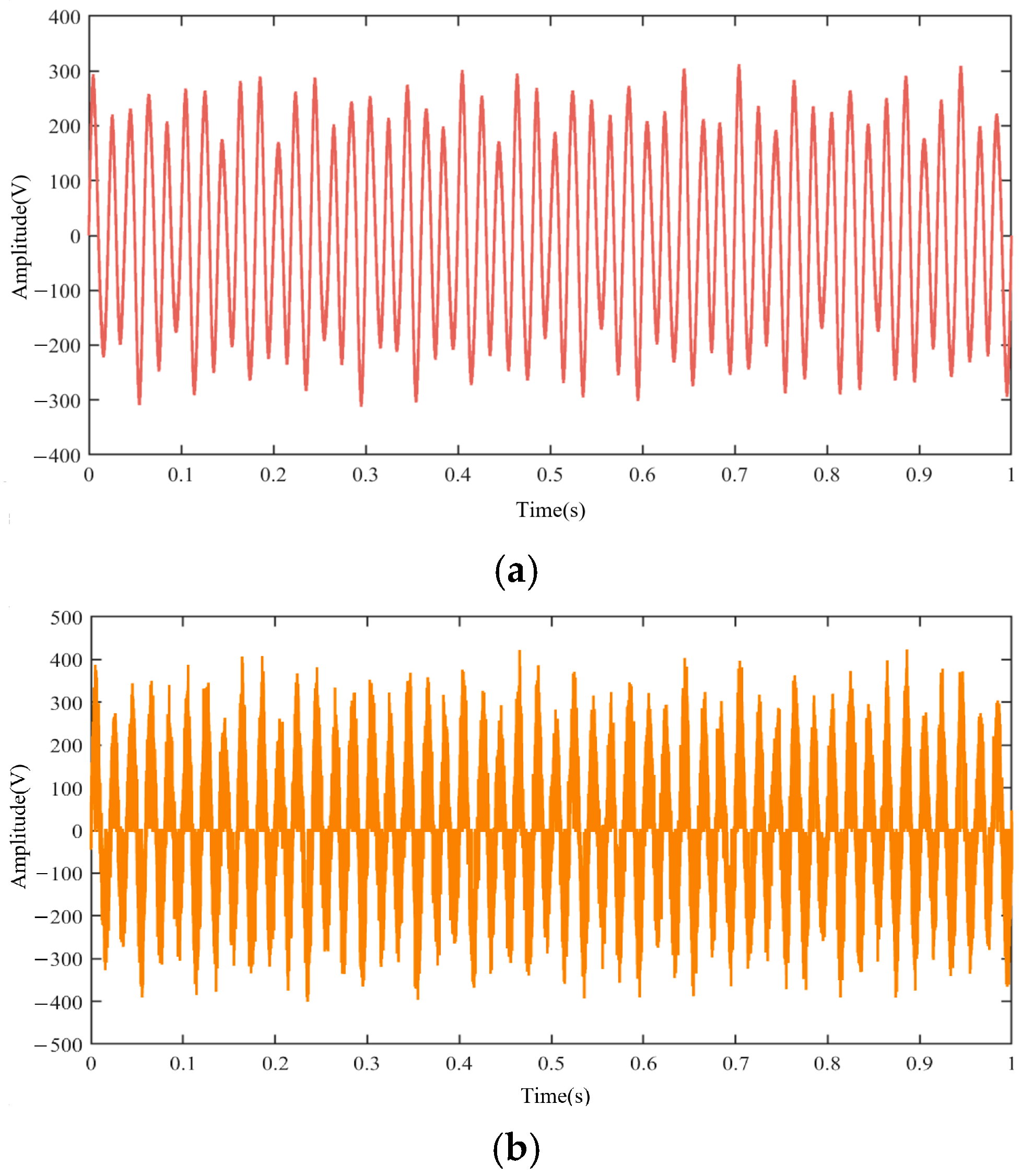
To establish the test signal shown in (33), the test signal consists of the original signal and noise. Considering the wide frequency distribution of broadband oscillation and the possibility of containing multiple oscillation components, the original signal contains four broadband oscillation frequencies, 33 Hz, 87 Hz, 246 Hz and 1500 Hz, in addition to the fundamental frequency 50 Hz, and the oscillation amplitude is generated randomly. The noise contains Gaussian white noise and background noise, where N_G(t) adds Gaussian white noise with a signal-to-noise ratio of 10 dB, and N_P(t) adds random impulse noise with an amplitude four times that of the background noise, and the random impulse noise is set to have a coverage of 5% in the time domain. The sampling frequency is set to 10 kHz and the time length of monitoring data is set to 1 s. The test signal model used is as follows:

$$x(t)=x_1(t)+x_N$$

(33)

$$\left\{\begin{array}{l}{x}_1(t)=220\cos (2\pi 50t)+50\cos (2\pi 33t)+25\cos (2\pi 87t)\\ \hspace{1em}\hspace{1em}\hspace{1em}+20\cos (2\pi 246t)+\cos (2\pi 1500t)\\ x_N=N_G+N_P\end{array}\right.$$

(34)

In (34), x₁(t) is the original signal, x_N is the noise, and N_G and N_P are Gaussian white noise and impulse noise, respectively.

The waveforms of the original signal without noise and the test signal containing noise are shown in Figure 3a,b, respectively. From the figures, it can be visualized that the test signal has random fluctuations superimposed on the original signal, indicating that the noise interferes seriously with the test signal.

Using the SLST wavelet denoising method proposed in this paper, the test signal is denoised. According to the noise characteristics of the test signal (Gaussian white noise with an SNR of 10 dB and impulse noise with 5% coverage), the Bayes threshold method is used to calculate the lower threshold, λ₁ = 0.4. The upper threshold λ₂ is set to 0.6 to ensure the effective retention of signal features (such as low-amplitude components at 1500 Hz) in the smooth transition region while suppressing noise interference. The noise-reduced test signal is compared with the original signal without noise, and the original signal and the denoised signal are compared as shown in Figure 4.

As can be seen from Figure 4, the denoised signal and the original signal not only fit well on the overall waveform, but also fit relatively well on the local waveform, indicating that the wavelet noise reduction method proposed in this paper can effectively eliminate the noise and retain the effective information of the original signal.

To evaluate more specifically the noise reduction effect of the designed method on test signals containing noise, the Pearson Correlation Coefficient and the SNR are used as the evaluation indexes.

$$r={\displaystyle \frac{{\displaystyle \sum _{i=1}^n}\left(S_{n,i}-S_{n,m}\right)\left(S_{de,i}-S_{de,m}\right)}{\sqrt{{\displaystyle \sum _{i=1}^n}{\left(S_{n,i}-S_{n,m}\right)}^2}\sqrt{{\displaystyle \sum _{i=1}^n}{\left(S_{de,i}-S_{de,m}\right)}^2}}}$$

(35)

.

$$SNR=10\cdot {\log }_{10}{\displaystyle \frac{{‖S‖}_2^2}{{‖S-S_{de,m}‖}_2^2}}$$

(36)

In (35) and (36), S is the original signal without random noise interference, S_n is the signal after adding noise interference, S_de is the signal after noise reduction, S_n,m and S_de,m are the mean value of the signal with noise interference and the noise reduction signal, and n is the length of the signal. The value of the Pearson correlation coefficients ranges from −1 to 1. A Pearson correlation coefficient close to 1 indicates a high degree of correlation between the noise-reduced signal and the original signal, suggesting a superior noise reduction effect. Conversely, a value close to −1 implies a strong negative correlation, while a value of 0 indicates no linear correlation. Additionally, a higher SNR corresponds to lower noise content and a better noise reduction outcome.

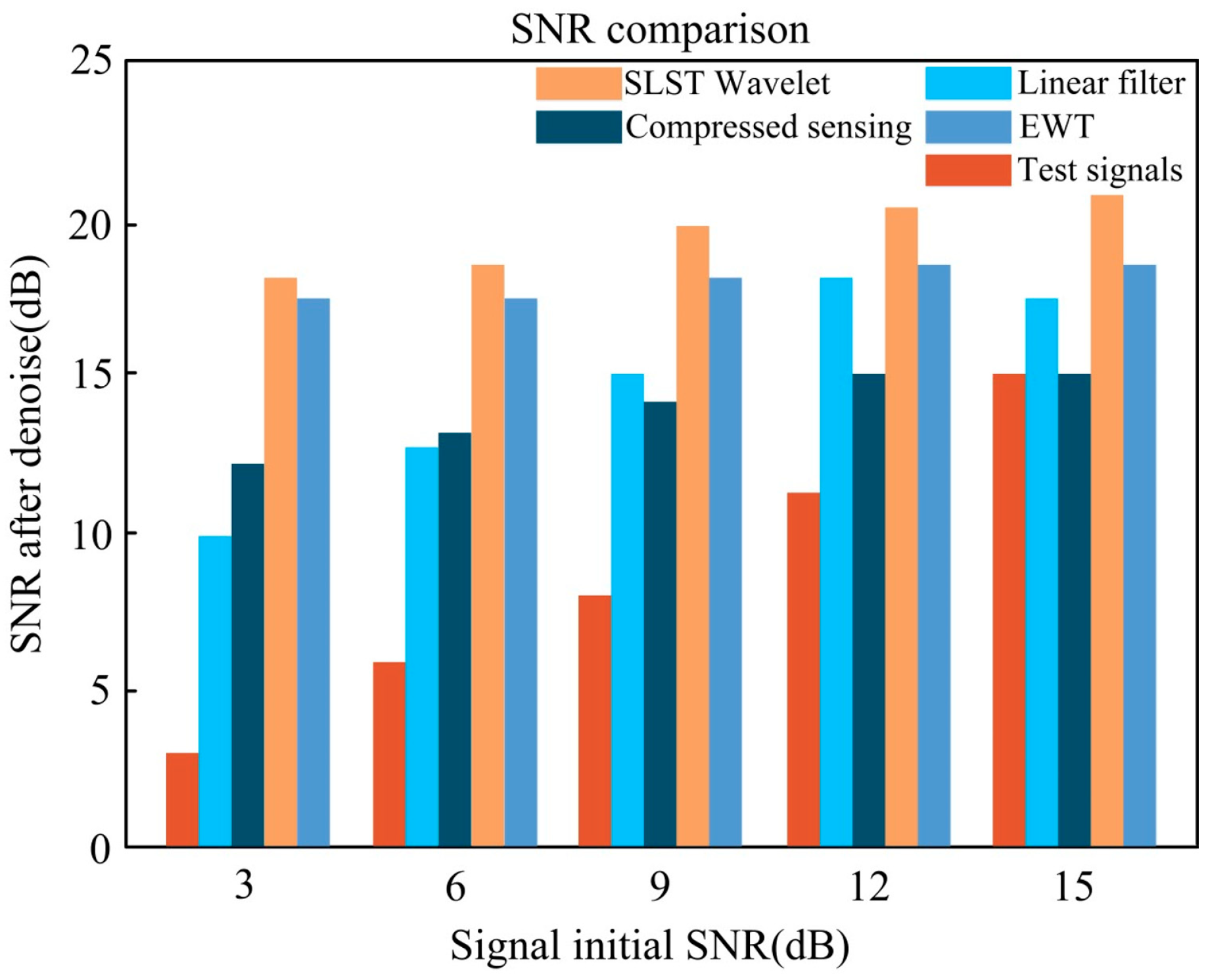
To verify the advantage of SLST wavelet denoising proposed in this paper over other types of noise removal methods in terms of noise removal effect, the test signals are analyzed and compared with linear filtering, compression-aware and Empirical Wavelet Transform (EWT) methods. As shown in Figure 5, the SLST wavelet denoising method proposed in this paper has the best noise reduction effect.

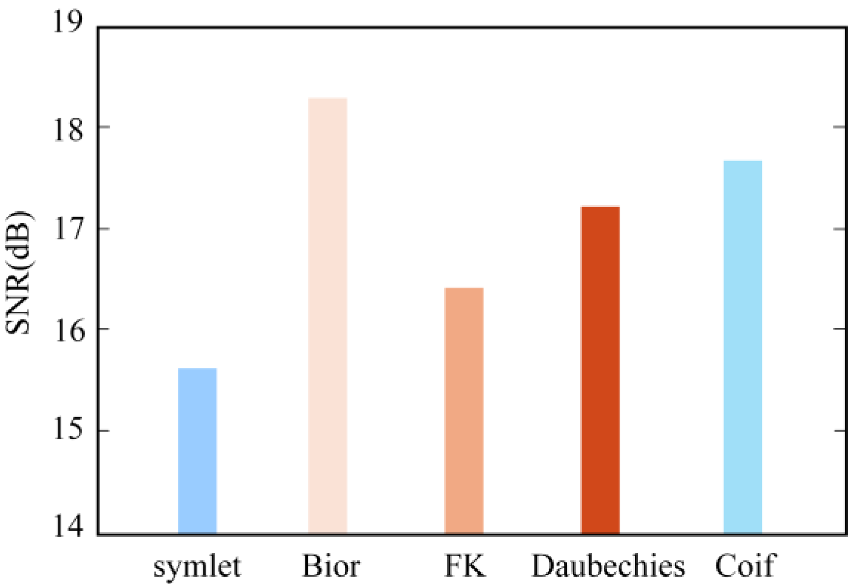
To verify the reasonableness of choosing the Bior wavelet basis function for SLST wavelet noise reduction, we applied five different wavelet basis functions, namely, symlet, Bior, Fejér-Korovkin (FK), Daubechies and Coiflet (Coif), to the test signals for noise reduction. By comparing and analyzing the noise reduction effect of each wavelet basis function, it can be intuitively found in Figure 6 that the Bior wavelet basis function shows certain advantages in noise reduction performance compared with other types of wavelet basis functions.

To further verify the noise reduction effect of the method proposed in this paper, the test signals are analyzed and compared with the three wavelet noise reduction methods using HT, ST and the SLST proposed in this paper, respectively.

The SNR and Pearson’s coefficient of the test signal before noise reduction are 8.38 and 0.9291, respectively, and the results of the SNR and Pearson’s coefficient of the test signal after noise reduction with the three wavelet noise reduction methods, respectively, are shown in Figure 7.

From Figure 7, we can see that using the wavelet denoising method with SLST wavelet denoising method proposed in this paper, the Pearson’s coefficient takes a value closer to 1 and the SNR takes a larger value relative to the HT and ST, which indicates that after using the noise reduction method in this paper, the noise reduction signal has a higher correlation with the original signal, and the noise reduction effect is better.

The results of the quantitative comparison of different thresholding methods are given in

Table 1. Noise reduction effect of different wavelet denoising methods.

Thresholding Methods	SNR	Pearson’s Coefficient
HT	16.78	0.9901
ST	17.40	0.9920
SLST	18.30	0.9936

. From Table 1, we can see that after using three different threshold wavelet noise reduction methods, the SNR of denoised signals is improved by 8.4, 9.02, and 9.92, respectively. The SNR of denoised signals is improved by 0.061, 0.0629, and 0.0645, respectively. The SLST wavelet denoising method proposed in this paper has the best performance in the evaluation indexes of the noise reduction effect, which is more suitable for the application in high-noise broadband signals.

4.2. Broadband Signal Simulation Test

The test signal consists of a fundamental frequency signal and an oscillating signal within the 2.5–1000 Hz range. In the previous section, we verified that after preprocessing of noise reduction of the broadband signal, the interference noise is removed with good effect, and the effective information of the signal is retained intact, so for the simplification of the simulation test, the existence of noise interference of the signal is not considered.

To verify the decomposition effect of the VMD and the accuracy of Prony parameter identification, the test signal of (37) is constructed. Considering the wide range of broadband oscillation frequency distribution and the possibility of multiple oscillation components, four broadband oscillation frequencies are generated in addition to the fundamental frequency of 50 Hz, and the amplitude of oscillation is generated randomly. The signal expression is as follows:

$$\begin{array}{c}x(t)=220\cos (2\pi \times 50t)+50\cos (2\pi \times 114t)\\ +20\cos (2\pi \times 295t)+10\cos (2\pi \times 780t)\end{array}$$

(37)

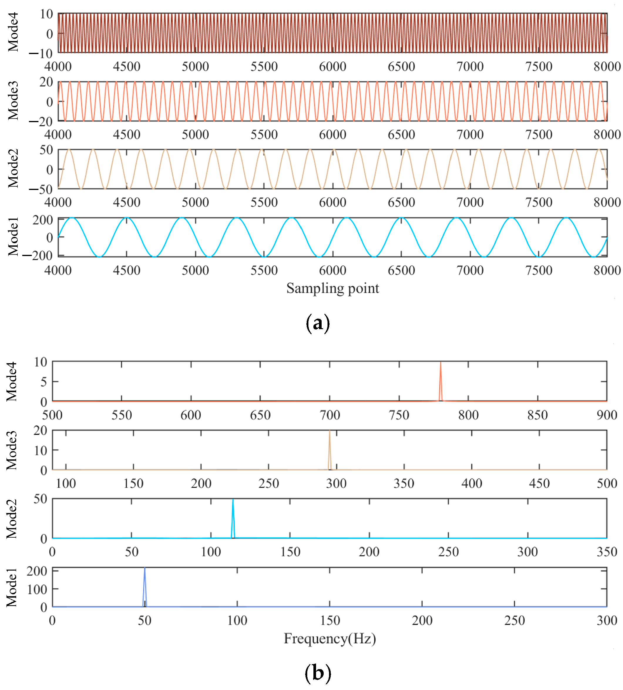
The mode decomposition of the above signal is carried out by using the parameter-optimized VMD. The modal number k is determined to be four by mutual information entropy optimization, matching on the four main frequency components of the test signal. The penalty factor α is determined by energy entropy minimization to be 2100. The VMD decomposition results are shown in Figure 8: Figure 8a shows the time-domain decomposition results of each mode, and Figure 8b shows the frequency-domain decomposition results of each mode. We can intuitively see that the method proposed in this paper can effectively separate the modes.

After mode decomposition of the signal by VMD, a complex signal can be decomposed into a series of modes, each of which represents a component of the signal in a different frequency band.

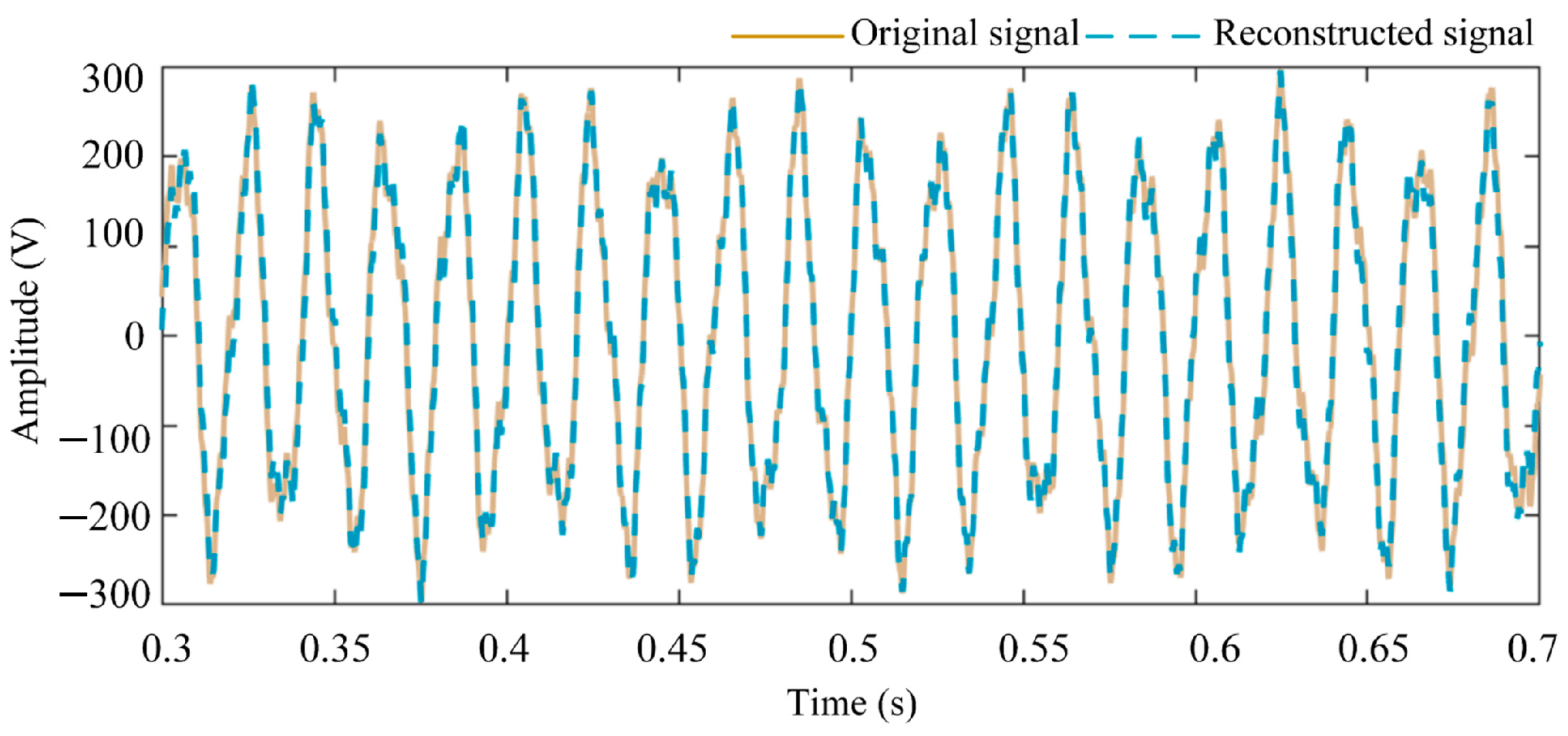
As shown in Figure 8b, each mode of the VMD decomposition contains a single center frequency and the number of significant frequency peaks N_peaks is 1. Therefore, for each mode, the model order p is set to 2. Prony recognizes the information of each mode parameter and linearly combines all modes to obtain the reconstructed signal. As shown in Figure 9, the original signal fits well with the reconstructed signal, indicating that the parameter identification of the signal is relatively accurate.

After the mode decomposition of the signal by VMD, the amplitude, phase, frequency information and relative error percentage of each mode are identified by Prony as shown in

Table 2. Theoretical and identified values of each modal parameter and percentage of relative error.

Mode	Parameter	Theoretical Value	Identified Value	Percentage of Relative Error
1	Amplitude/V	220	219.4030	0.2713
	Frequency/Hz	50	50	0
2	Amplitude/V	50	49.3945	1.2110
	Frequency/Hz	114	114	0
3	Amplitude/V	20	19.8867	0.5665
	Frequency/Hz	295	295	0
4	Amplitude/V	10	9.98117	1.883
	Frequency/Hz	780	780	0

.

As can be seen from Table 2, the relative error between the frequency discrimination value and the theoretical value of each mode is 0, which proves that the frequency discrimination is excellent, and the relative error percentages between the amplitude discrimination value and the theoretical value of mode 1, mode 2, mode 3 and mode 4 are 0.271%, 1.2210%, 0.5665%, 0.1.883%, respectively, and the deviation of the discrimination value and the theoretical value can be approximately neglected. This shows that the parameter identification of the signal is relatively accurate.

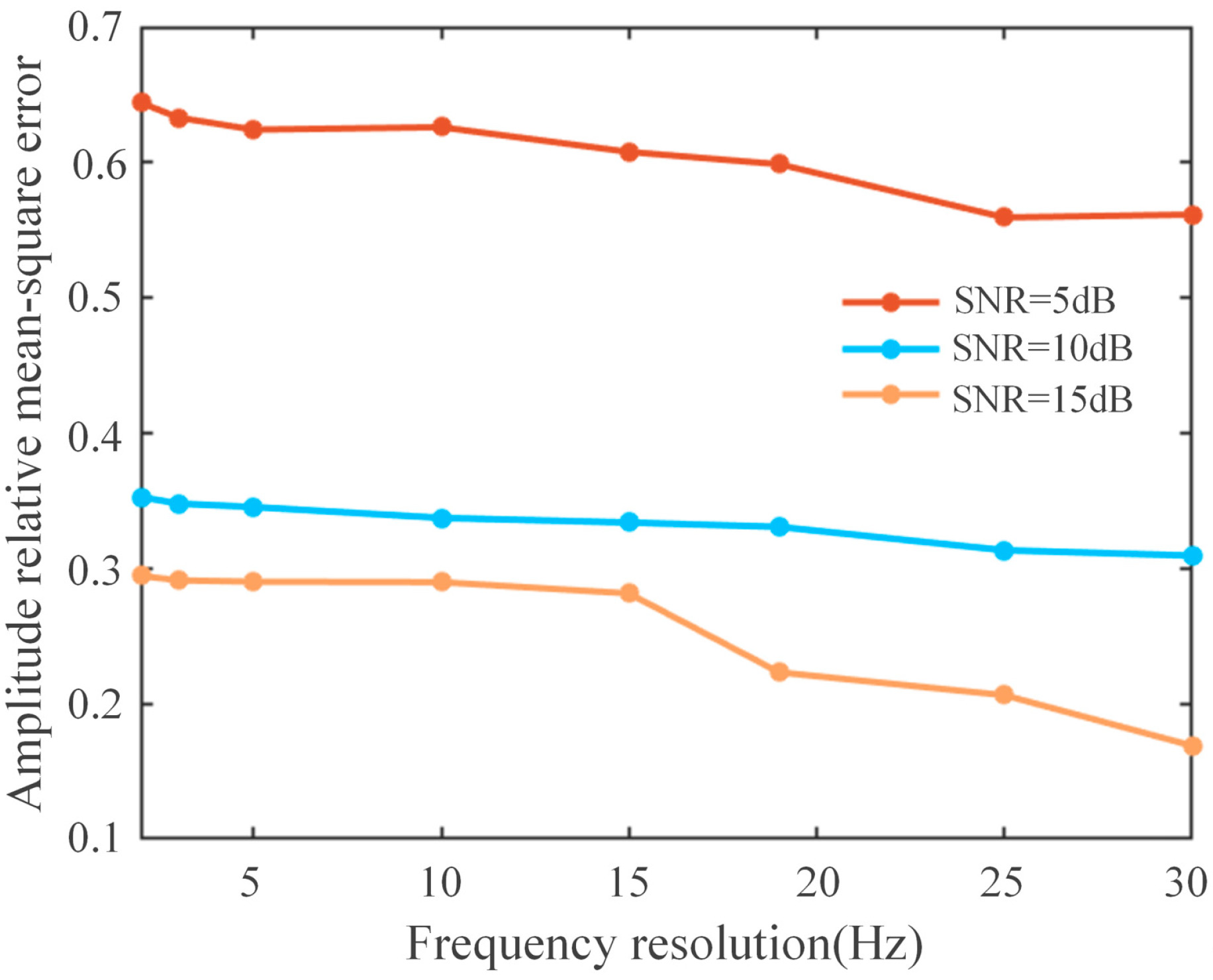
To demonstrate the effectiveness of the proposed method in noise reduction and accurate measurement, several typical broadband measurement algorithms, including EMD, FFT, ESPRIT, MUSIC and Prony, were selected for comparative analysis. Specifically, EMD was configured to extract four IMFs: FFT utilized a 1024-point Hamming window, and ESPRIT, MUSIC, and Prony all employed a model order of ten. These parameter settings were optimized through preliminary experiments to ensure a fair and comprehensive evaluation of performance. To investigate the signal reconstruction results of different methods at different noise levels and different frequency intervals, the test simulation results of amplitude are shown in Figure 10.

As can be seen in Figure 10, the FFT consistently exhibits high RMSE values, approximately 3.0, due to its sensitivity to noise, spectral leakage, and limited frequency resolution. EMD reduces processing complexity by decomposing signals into IMFs. When the SNR increases from 5 dB to 30 dB, its RMSE shows a modest decline from 1.2 to 1.0, indicating that a higher SNR mitigates noise interference in mode decomposition. However, inherent issues like mode mixing and end effects prevent EMD from accurately separating closely spaced frequency components, resulting in high RMSE values. The ESPRIT algorithm demonstrates a moderate improvement, with RMSE decreasing from 1.5 to 1.3 as SNR rises and the frequency spacing widens. Yet, under high noise or narrow frequency intervals, its subspace decomposition becomes vulnerable to noise, limiting resolution and maintaining higher errors. Although Prony’s method is noise sensitive, with its linear prediction coefficients prone to distortion, it achieves greater robustness for test signals with distinct frequency components through direct fitting, stabilizing RMSE at approximately 1.0 and outperforming ESPRIT in this scenario. MUSIC exhibits an extremely high-frequency resolution. However, under low SNR conditions, noise significantly interferes with subspace decomposition. As the SNR increases from 5 dB to 30 dB, the RMSE of MUSIC decreases markedly. The proposed algorithm in this study demonstrates remarkable superiority, maintaining RMSE consistently below 0.6. As illustrated in Figure 11, its RMSE decreases significantly with increasing SNR and frequency spacing, with a minimum RMSE of 0.17. These results conclusively validate the algorithm’s exceptional noise suppression capability and high-frequency resolution performance.

4.3. Hardware-in-the-Loop Simulation Testing

To verify the applicability of the broadband oscillation measurement algorithm proposed in this paper in the real power system, the simulation arithmetic of the PV grid-connected system is constructed, as shown in Figure 12. The circuit parameters for the PV grid-connected model are detailed in

Table 3. Circuit parameters of the simulation model.

Parameter	Symbol	Value
DC voltage	Vdc	700 V
Grid voltage amplitude	V1	311 V
Filter inductor	Lf	4 mH
Filter capacitor	Cf	20 μF
Damping resistor	Rf	1.3 Ω
Switching frequency	fs	20 kHz
Current PI controller proportional gain	kp	0.0324
Current PI controller integral gain	ki	44.7225
Voltage feedforward coefficient	Kf	0.0028
Feedforward decoupling gain coefficient	Kd	0.0030

.

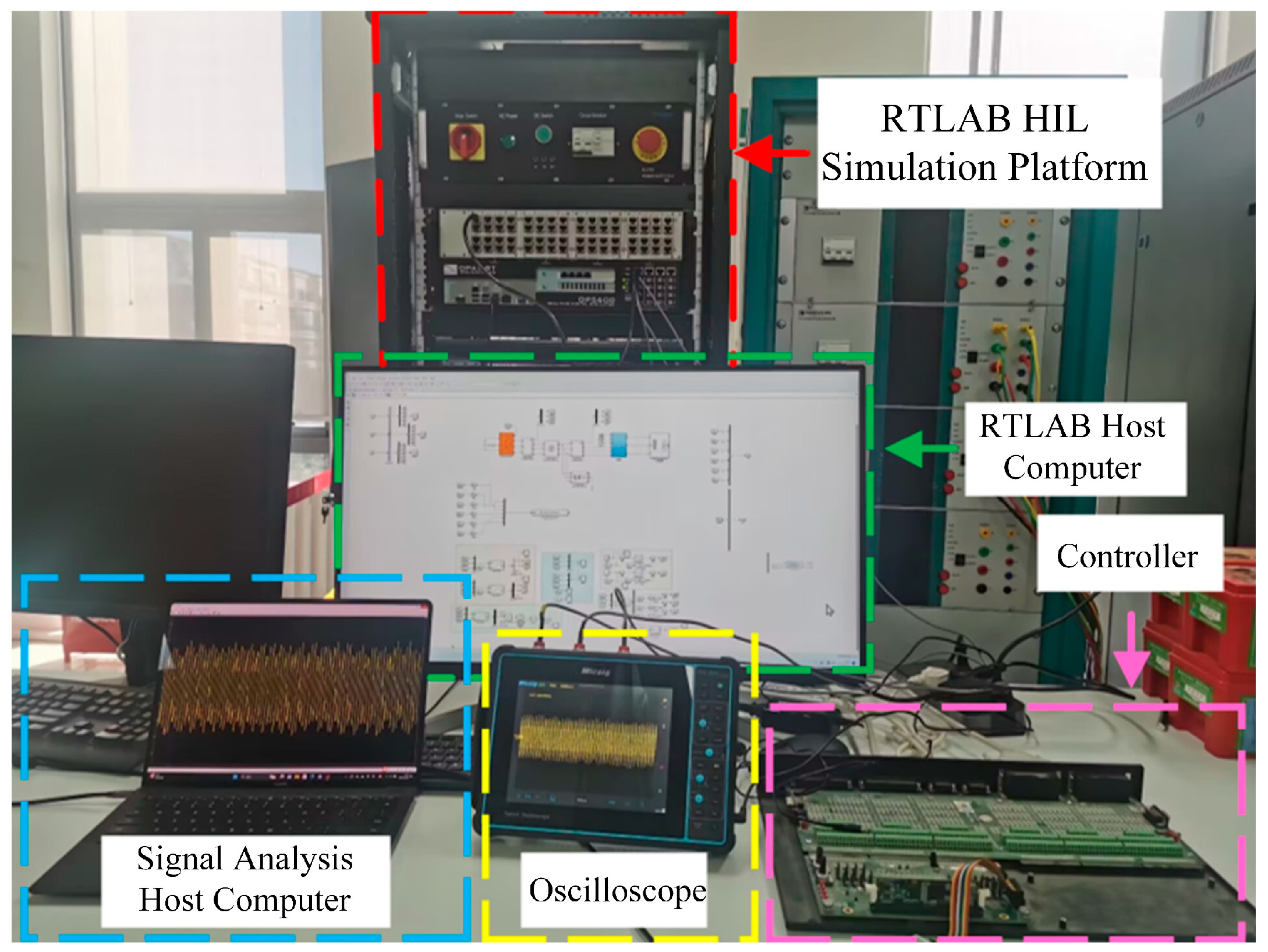
As shown in Figure 13, a RTLAB Hardware-in-the-Loop (HIL) simulation platform was constructed. The platform consists of RTLAB, an RTLAB host computer, a controller, an oscilloscope and a signal analysis host computer. RTLAB can compile and simulate the PV grid-connected model in Simulink and perform an HIL simulation by interacting with external hardware circuits through the IO boards and FPGAs carried in the machine. In the experiment, by adjusting the parameters of the PV grid-connected inverter controller and line impedance parameters to make its AC side generate the expected broadband oscillating signals to simulate the dynamic behavior of the signal source, and then synchronously collect and process the voltage and current signals, and input the collected data into the proposed broadband measurement algorithm model for measurement.

The platform consists of RTLAB, an RTLAB host computer, a controller, an oscilloscope and a signal analysis host computer. RTLAB can compile and simulate the PV grid-connected model in Simulink, and perform an HIL simulation by interacting with external hardware circuits through the IO boards and FPGAs carried in the machine. In the experiment, by adjusting the parameters of the PV grid-connected inverter controller and line impedance parameters to make its AC side generate the expected broadband oscillating signals to simulate the dynamic behavior of the signal source, and then synchronously collect and process the voltage and current signals, and input the collected data into the proposed broadband measurement algorithm model for measurement.

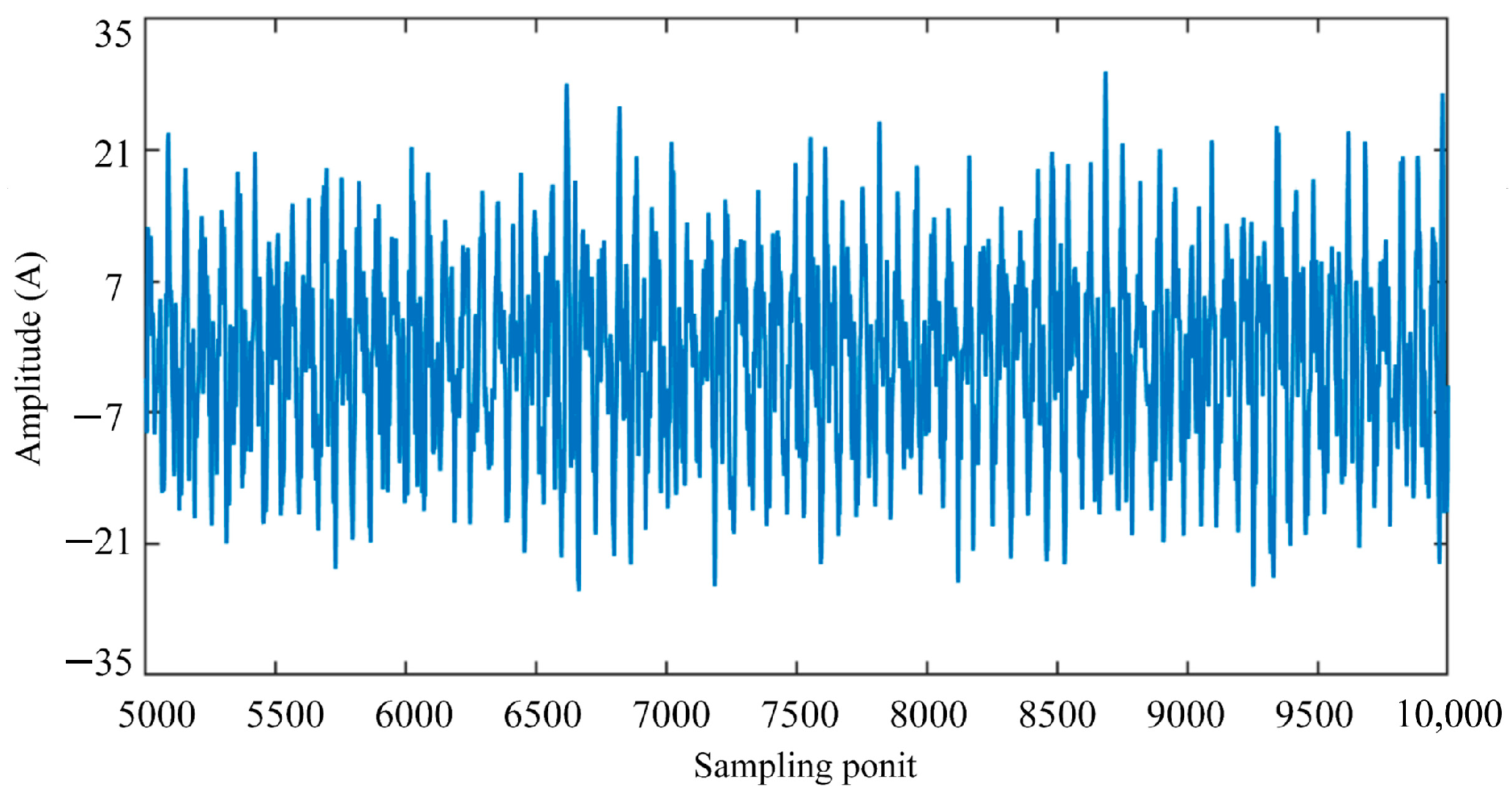
Phase A current i_a is selected as the signal to be analyzed, and the current signal on the oscilloscope is captured, and its oscillating waveform is shown in Figure 14.

Because of the need to verify that the broadband measurement algorithm in this paper can reduce noise interference, the simulation example artificially adds a noise source. According to the oscillating signal data shown in Figure 14, the noise reduction preprocessing is carried out on the broadband signal by using the SLST wavelet denoising method, and the noise-reduced signal is decomposed by the parameter-optimized VMD, which decomposes multiple modes, as shown in Figure 15.

From Figure 15, we can see that the five main modes are decomposed, containing one fundamental frequency mode and four main oscillatory modes of the system. The Prony is used to identify the parameters of each mode after the VMD decomposition, and the frequency, amplitude, and phase parameter information of the center of each mode is obtained as shown in

Table 4. Frequency, amplitude, and phase parameter information for each mode center.

Mode	Frequency/Hz	Amplitude/A	Phase/Rad
1	636.2143	0.8914	0.5903
2	475.1396	1.1833	−2.9985
3	319.9806	1.2821	0.8513
4	163.6722	3.7035	−1.5546
5	50.0727	20.0593	0.2566

.

Since the real parameter information of the A-phase current signal is unknown, the current signal reconstruction is realized by linear combination of the modal parameter information obtained by identification, and the effectiveness of the algorithm proposed in this paper on the accurate measurement of the signal is verified by comparing the fitting degree of the collected original current signal and the reconstructed signal. To compare the original current signal with the reconstructed signal more intuitively and clearly, the comparison graph is locally enlarged, as shown in Figure 16.

From Figure 16, we can see that the reconstructed signal is basically consistent with the original signal waveform and the fitting degree is high, which verifies that the proposed algorithm can make an accurate measurement of the signal and effectively obtain the relevant parameter information of the oscillating signal.

4.4. Actual Recorded Wave Data Testing

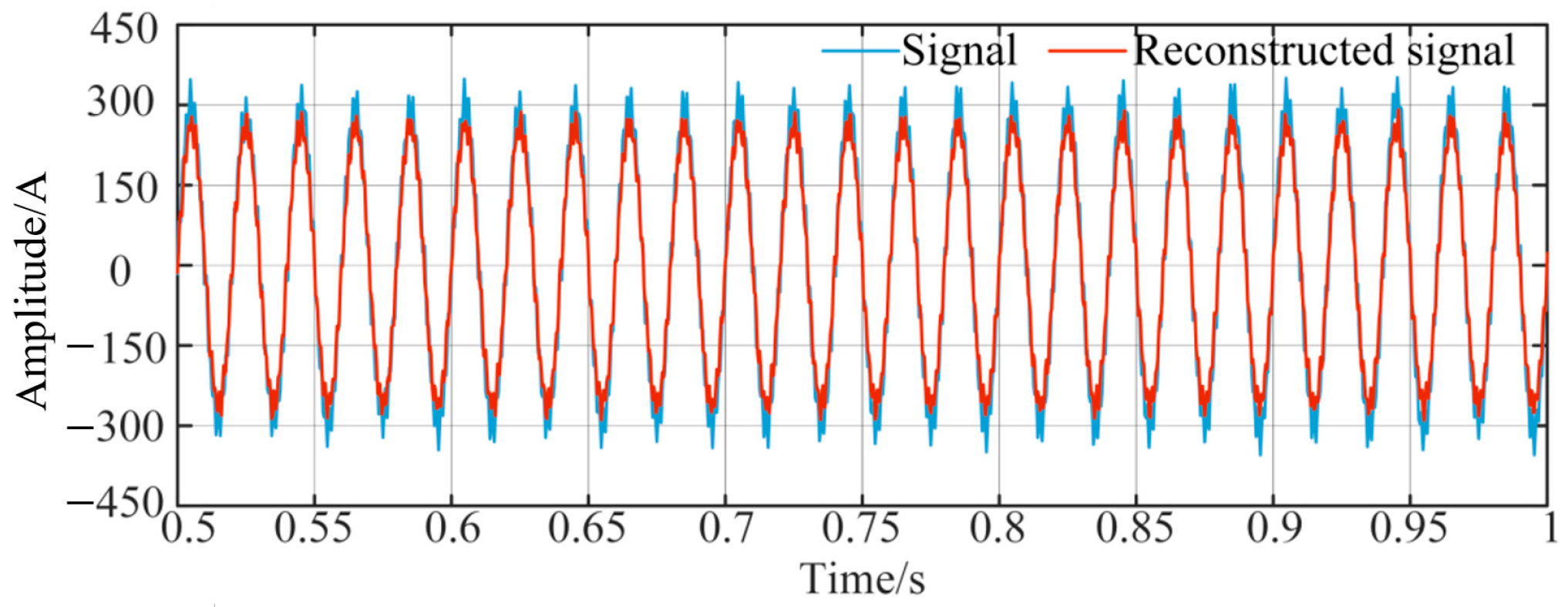
The effectiveness of the proposed method is verified based on the fault recording data of a 35 kV photovoltaic power station under the jurisdiction of a substation in Ningxia, China. The waveform of the A-phase current recording data of the 35 kV busbar is shown in Figure 17, and the current signal consists of a fundamental component, a sub-synchronous component with a frequency of 31 Hz, a component with a larger amplitude of 69 Hz, and some harmonic interferences with smaller amplitudes.

The coefficient of determination R² was chosen as an index for evaluating the measurement results, and was used to measure the difference between the reconstructed signal and the original signal, the closer R² is to 1, the better the reconstructed signal fits the original signal. The closer R² is to 1, the better the reconstructed signal fits the original signal, and the more accurate the proposed broadband oscillation signal measurement method is. The range of R² is from 0 to 1, and R² ≥ 0.9 is usually taken as the criterion of high precision fitting, and the specific formula is as follows.

$$R^2=1-{\displaystyle \frac{{\displaystyle \sum _{i=1}^n}{(x_i-{\widehat{x}}_i)}^2}{{\displaystyle \sum _{i=1}^n}{(x_i-\overline{x})}^2}}$$

(38)

where n is the number of data points, x_i is the ith value of the original signal, ${\widehat{x}}_i$ is the ith value of the reconstructed signal, and $\overline{x}$ is the mean value of the original signal.

Using the proposed method to measure the current signal, the reconstructed signal and the original signal comparison chart are shown in Figure 18, which can be visualized that the reconstructed signal and the original signal waveform is basically consistent and high degree of fit. In addition, the calculated R² value of the reconstructed signal to the original voltage signal is 0.925, which exceeds the criterion for high-precision fitting, further indicating that the proposed method can realize the accurate measurement of the signal.

5. Discussion

The proposed algorithm combines SLST wavelet denoising, optimized VMD, and Prony-based parameter identification to address noise interference and measurement inaccuracies in broadband signal analysis. The SLST method introduces a smooth transition zone between thresholds, effectively preserving signal features while suppressing noise. In tests with mixed Gaussian and impulse noise, SLST improved the SNR by 118% (from 8.38 to 18.30) and Pearson’s correlation to 0.9936, outperforming hard/soft thresholding by 9–18% in denoising efficiency. The dual-entropy optimized VMD (k = 4, α = 2100) achieved precise decomposition of four frequency signals with negligible aliasing. Subsequent Prony analysis achieved perfect frequency detection and kept amplitude errors below 1.9%, reducing RMSE by over 50% compared to conventional methods. Through HIL simulations and field testing on a 35 kV PV system, the algorithm demonstrated excellent waveform fidelity, achieving a coefficient of determination R² of 0.925 between the original and reconstructed signals, validating the algorithm’s effectiveness for power system broadband oscillation analysis.

However, the algorithm’s computational complexity, driven by VMD and Prony iterations, increases with signal frequency complexity or higher sampling rates, limiting real-time performance for long-term monitoring. Future work will explore advanced decomposition techniques, such as ICEEMDAN, to enhance noise robustness and decomposition accuracy for complex signals. Additionally, optimizing computational processes and leveraging hardware acceleration, such as GPUs or FPGAs, will be investigated to improve real-time processing in practical applications.

6. Conclusions

In this paper, a broadband measurement algorithm based on SLST wavelet denoising and improved VMD-Prony is proposed, and its effectiveness is verified by simulation tests. The main conclusions are as follows:

The SLST wavelet denoising method can effectively remove the noise interference, retain the effective information of the signal, and improve the signal quality. Compared with the hard threshold and soft threshold methods, the noise reduction method proposed in this paper performs better in terms of signal-to-noise ratio and Pearson’s correlation coefficient and can better adapt to the broadband signal noise reduction needs in the high-noise environment.

The improved VMD can decompose the broadband signal into multiple modes with center frequencies, which reduces the complexity of signal processing and improves the decomposition accuracy. Optimizing the VMD parameters by mutual information entropy and energy entropy can effectively avoid the phenomenon of modal aliasing and improve the accuracy of signal decomposition.

The algorithm proposed in this paper can accurately identify the parameters of each mode, obtain the frequency, amplitude, phase and other parameter information of each mode, and performs better in amplitude identification accuracy and frequency resolution compared with the traditional methods of EMD, FFT and ESPRIT.

The broadband measurement algorithm proposed in this paper has achieved good results in simulation tests and HIL simulation tests, and can be effectively applied to the analysis of broadband oscillations in power systems, providing important technical support for the safe and stable operation of power systems.