Spatial-Temporal Traffic Flow Prediction Through Residual-Trend Decomposition with Transformer Architecture

Abstract

Accurate traffic forecasting is challenging due to the complex spatial-temporal interdependencies of large road networks and sudden speed changes caused by unexpected events. Traditional models often struggle with the non-stationary and volatile characteristics of traffic time series. While existing sequence decomposition methods can capture stable long-term trends and periodic information, they fail to address complex fluctuation patterns. To tackle this issue, we propose the Spatial-Temporal traffic flow prediction with residual and trend Decomposition Transformer (STDformer), which decomposes time series into different components, thus enabling more accurate modeling of both short-term and long-term dependencies. Our method processes the time series in parallel using the Trend Decomposition Block and the Spatial-Temporal Relation Attention. The Spatial-Temporal Relation Attention captures dynamic spatial correlations across the road network, while the Trend Decomposition Block decomposes the series into trend, seasonal, and residual components. Each component is then independently modeled by the Temporal Modeling Block to capture its unique temporal dynamics. Finally, the outputs from the Temporal Modeling Block are fused through a selective gating mechanism, combined with the Spatial-Temporal Relation Attention output to produce the final prediction. Extensive experiments on PEMS traffic datasets demonstrate that STDformer consistently outperforms state-of-the-art traffic flow prediction methods, particularly under volatile conditions. These results validate STDformer’s practical utility in real-world traffic management, highlighting its potential to assist traffic managers in making informed decisions and optimizing traffic efficiency.

1. Introduction

Traffic forecasting is a critical task in time series analysis, with wide-ranging applications in urban planning, congestion management, and route optimization. Despite its practical significance, accurately predicting traffic flow remains challenging due to the complex spatio-temporal dependencies inherent in road networks. Unlike conventional time series problems, traffic data exhibits dynamic interactions across multiple locations, where conditions on one road segment nonlinearly influence others. These dependencies are further complicated by external factors such as weather disruptions, accidents, and periodic events (e.g., holidays) [1,2,3], demanding robust modeling approaches.

As a prominent real-world application of multivariate time series (MTS), traffic flow prediction poses unique challenges in modeling temporal dependencies within individual sequences and spatial correlations between them. On one hand, the spatial dimension requires capturing diverse traffic patterns among nodes in road networks, which often form intricate, non-Euclidean structures [4]. On the other hand, the temporal dimension involves learning both short-term fluctuations (e.g., abrupt congestion from accidents) and long-term trends (e.g., daily commute peaks or seasonal demand shifts) [5]. Traffic flow refers to the number of vehicles passing a specific point in a unit of time, while traffic speed indicates the speed of vehicles on the road. These metrics are crucial for analyzing and optimizing traffic management, as they directly influence congestion levels and overall traffic efficiency [6]. Moreover, traffic flow data represents a spatiotemporal sequence, integrating both spatial and temporal aspects to provide a comprehensive understanding of traffic dynamics.

Recent research has made significant progress in addressing these challenges. Traditional statistical methods like ARIMA [7,8] and its variants (e.g., SARIMA [9]) have proven inadequate for handling the non-stationary and nonlinear nature of traffic data, particularly when modeling large-scale networks [10]. Early machine learning approaches, including support vector regression (SVR) [11] and random forests [12], showed improved performance but often failed to capture complex spatial relationships between road segments. To overcome the challenges related to spatio-temporal modeling, many deep learning models have been proposed, including graph convolutional networks (GCNs), recurrent neural networks (RNNs), and Transformer. Graph neural networks (GNNs) like STGCN [13,14] effectively model road network structures using graph convolution operations, outperforming traditional methods, such as ARIMA. Existing deep learning models, such as graph convolutional networks (GCNs) and recurrent neural networks (RNNs), typically treat spatial correlations in a static manner, lacking the ability to dynamically adapt to varying traffic conditions. This limitation hinders their effectiveness in accurately modeling the intricate interactions among traffic nodes. Recurrent architectures [15] handle temporal dependencies but suffer from error accumulation in long sequences. More recently, transformer-based models like ASTGNN [16] and STGTN [17] have demonstrated superior capability in capturing long-range temporal dependencies through self-attention mechanisms. Recent research has made significant progress in addressing these challenges; for instance, a study proposed a vessel traffic flow prediction method using an origin-destination (O-D) matrix and a Spatio-Temporal Zero-Inflated Negative Binomial Graph Neural Network (STZINB-GNN) [18], effectively modeling internal coupling relationships within traffic networks and demonstrating superior accuracy in predicting vessel traffic flow. However, these models still face significant challenges in fully addressing the intricate spatial correlations between traffic nodes. They often assume static relationships, which limit their responsiveness to real-time traffic conditions and dynamics.

Motivated by the aforementioned observations, we propose a traffic flow prediction model from a decoupling perspective, namely STDformer. For the temporal correlations within time series, we decouple the data into trend, seasonal, and residual parts, using Vanilla Transformer, Fourier attention mechanism, and Multi-layer Perceptron (MLP), respectively. For the spatial correlations among time series, we utilize the inverted transformers, which leverage the geographical adjacency relationships of the road network to capture the pattern correlations between traffic flow nodes. Our main contributions are summarized as follows:

• Our STDformer proposes a decomposition module using Fast Fourier Transform (FFT) and Inverse Fast Fourier Transform (IFFT) to extract trend, seasonal, and residual components, better to capture long-range correlations from a decoupling perspective. The Temporal Modeling Block captures the historical traffic flow patterns among different nodes. An adaptive gating mechanism dynamically weights these components, enhancing prediction accuracy.
• STDformer tailors specific approaches for each component, utilizing a Transformer model to effectively capture the trend, employing frequency-enhanced attention to analyze seasonality, and applying RevIN-MLP to model the residuals. The Spatial-Temporal Relation Attention mechanism captures relationships among traffic nodes, enabling unified temporal and spatial modeling. We design a Spatial-Temporal Relation Attention mechanism that captures relationships among traffic nodes, enabling unified temporal and spatial modeling.

In the rest of this paper, we first review the related work in Section 2. The details of the proposed STDformer framework are discussed in Section 3, followed by the results of the experimental evaluations highlighting the advantages of our approach in Section 4. In Section 5, we provide a comprehensive analysis of the results. Finally, in Section 6, we conclude the study and outline future directions.

2. Related Work

2.1. Deep Learning-Based Traffic Forecasting

Deep learning models have achieved significant success in traffic forecasting by effectively capturing spatio-temporal features. Convolutional Neural Networks (CNNs) have been widely used for spatial modeling, particularly in Euclidean spaces. For example, Zhang et al. [19] introduced a CNN-based method that effectively captures spatial correlations. However, CNNs have limitations when dealing with complex road networks, as they often require a fixed grid structure and may struggle to adapt to irregularities in spatial data. To address these challenges, Graph Neural Networks (GNNs) have gained popularity for modeling complex road networks. GNNs can represent spatial relationships more flexibly by utilizing graph structures, allowing for better handling of irregular topologies. The Graph Attention Network (GAT) [20] further enhances this capability by calculating attention coefficients for neighboring nodes, thereby extracting spatial correlations more effectively. Despite these advancements, GNNs still face issues with inaccurate predictions due to abrupt speed changes, instability, and evolving spatial dependencies.

In recent years, Transformer-based models have emerged as a powerful alternative, demonstrating even more competitive performance in long-term time series forecasting [21,22]. Their ability to capture long-range dependencies and dynamic relationships makes them particularly suited for spatio-temporal modeling in traffic forecasting. By leveraging attention mechanisms, Transformers can better navigate the complexities of traffic data, ultimately improving prediction accuracy.

2.2. Decomposition-Based Time Series Forecasting Methods

Decomposition techniques have gained significant attention in time series forecasting due to their ability to break down complex time series data into more interpretable components. These methods are particularly useful in capturing distinct temporal patterns, such as trends and seasonality (e.g., STL decomposition [23]), which are often obscured in raw data. Several approaches in the literature have leveraged decomposition to enhance the predictive accuracy of time series models.

Autoformer [24] employs a decomposition architecture that separates time series data into trend and seasonal components, using an Auto-Correlation mechanism to effectively capture long-term dependencies within each component. DLinear [25] utilizes simple moving averages for decomposition and models the decomposed trend and seasonal components using Multi-Layer Perceptrons (MLPs). Similarly, FEDformer [26] integrates frequency-enhanced decomposition techniques with transformers, applying seasonal-trend decomposition to disentangle global and local dependencies, thereby improving the model’s forecasting accuracy. Although these methods demonstrate the effectiveness of decomposition-based approaches, they share a common limitation: their reliance on simple moving average techniques for decomposition often fails to achieve precise component separation, particularly when handling complex and noisy real-world time series data where trend and seasonal components may not be clearly distinguishable. TimesNet [27] utilizes a modular structure to decompose complex time series variations into different periods, achieving unified modeling of intra-period and inter-period changes by transforming the original one-dimensional time series into a two-dimensional space. N-BEATS [28] employs low-degree polynomials to model trend components and utilizes Fourier series for the representation of seasonality. N-HiTS [29] extends the N-BEATS framework by refining input decomposition through the implementation of multi-rate data sampling, thereby enhancing its capability to capture complex temporal patterns. Similar to the findings of Han et al., effective data augmentation strategies could enhance model robustness in capturing these complexities [30]. While these methods demonstrate innovative approaches to time series modeling, their limitation is that the decomposition mechanisms employ static and non-adaptive operations that cannot automatically adjust to the variable periodicities and evolving patterns in real-world traffic data.

Decomposition techniques are particularly valuable in time series trend prediction, where time series data exhibit long-term trends and periodic variations. However, due to the multi-periodic nature and dynamic fluctuations of time series data, existing decomposition methods often fall short and cannot be directly applied to effectively capture the complexities inherent in time series trend prediction. Our proposed model, STDformer, advances the field by integrating a more comprehensive decomposition framework that captures multi-periodicity, cross-variable dependencies, and introduces a novel gating mechanism for dynamic feature fusion.

2.3. Fusion Methods in Time Series Forecasting

Fusion methods have emerged as a powerful approach in time series forecasting, particularly when dealing with complex datasets that exhibit multiple temporal patterns or sources of information. These methods aim to integrate various models, features, or data sources to enhance predictive performance by capturing complementary aspects of the time series data. H-MMoE enhances the efficiency and accuracy of multi-task learning by fusing multi-modal data [31]. The EMD-based method [32] combines the ARIMA model and neural network (NN) model through empirical mode decomposition and multiple model fusion, improving the prediction accuracy of chaotic time series.

TDformer [33] employs a simple additive fusion approach to combine the decomposed trend and seasonal components of the time series. In this method, the trend and seasonal components are modeled independently, and their outputs are summed to form the final prediction. While this additive method is straightforward and computationally efficient, it may not fully capture the intricate interactions between different temporal components, potentially limiting its effectiveness in scenarios where more complex relationships exist between trends and seasonality. PDF [34] employs a more advanced fusion method through its Variations Aggregation Block. After decomposing the time series into short-term and long-term variations, it processes these components separately and then sums their outputs. This fused representation is further refined by aggregating multiple outputs through a shared linear layer, enabling the model to capture and balance complex interactions between different temporal components for more accurate predictions.

Our proposed STDformer improves upon this by incorporating a gating mechanism that dynamically fuses the trend, seasonal, and residual components. This approach allows for a fine integration, where the influence of each component is weighted based on its relevance at each time step, leading to more accurate and robust predictions.

3. Framework of STDformer

First, let us define the time series prediction problem. We consider a traffic network comprising M regions or segments, with each region or segment containing a single traffic flow feature at each time step. We aim to predict the traffic flow for the next F time steps. For a specific region or segment, the input historical feature sequence is defined as $X_t=\{X_{t-T+1},X_{t-T+2},\dots ,X_t\}\in {\mathbb{R}}^{T\times M}$, where T represents the sequence length. The true labels for the next F time steps are represented as $Y_{t+1:t+F}=\{y_{t+1},y_{t+2},\dots ,y_{t+F}\}$, with $y_t$ denoting the actual traffic flow value at time step t. The prediction function for the traffic flow over the next F time steps can be expressed as ${\widehat{Y}}_{t+1:t+F}=f\left(X_{t-T+1:t}\right)$, where ${\widehat{Y}}_{t+1:t+F}$ indicates the predicted traffic flow values at time step t.

The overall architecture of our method is shown in Figure 1. STDformer aims to accurately model complex traffic patterns by first decoupling the traffic data to better handle variations. We design a Trend Decomposition Block to learn the periodicities of the input series in the frequency domain, along with the trend and residual components. The obtained seasonal, trend, and residual components are then fed into the Time Modeling Block, where we combine these components and apply a Gating Mechanism Fusion to dynamically adjust their contributions, ensuring each component’s influence is weighted based on its relevance at each time step. In parallel, the Spatial-Temporal Relation Attention mechanism operates alongside the Time Modeling Block to achieve end-to-end traffic flow prediction, allowing simultaneous processing of the decomposed components and spatial correlations in the traffic data. More details about our STDformer are provided in the following sections.

3.1. Trend Decomposition Block

The Trend Decomposition Block is designed to decompose the input time series into its fundamental components: trend, seasonal, and residual, as illustrated in Figure 2. This block comprises several key submodules: a Moving Average module for extracting trend components and the Seasonal Decomp Module for isolating seasonal patterns.

For a given input ${\mathbf{X}}_I\in {\mathbb{R}}^{T\times d}$ of dimension d, we employ a simple moving average to extract the trend components from the traffic data. Specifically, the moving average is adapted to smooth out periodic fluctuations and highlight the long-term trends. For a length-T input series $\mathbf{X}\in {\mathbb{R}}^{T\times d}$, the process is defined as follows:

$${\mathbf{X}}_t=\mathrm{AvgPool}\left(\mathrm{Padding}\left(\mathbf{X}\right)\right)$$

(1)

$${\mathbf{X}}_w=\mathbf{X}-{\mathbf{X}}_t$$

(2)

where ${\mathbf{X}}_w,{\mathbf{X}}_t\in {\mathbb{R}}^{T\times d}$ denote the preliminary component and the extracted trend component, respectively. We adopt the $\mathrm{AvgPool}(·)$ for moving average with the padding operation to keep the series length unchanged [24].

Previous work [33] only utilized the preliminary component ${\mathbf{X}}_w$ as the seasonal component for prediction, which was insufficient in capturing the full complexity and volatility of traffic data, particularly in effectively distinguishing between trend, seasonal, and residual influences.

To further decompose the preliminary component ${\mathbf{X}}_w$, unlike previous approaches that solely relied on ${\mathbf{X}}_w$ for the seasonal component, we enhance the process by applying the Fast Fourier Transform (FFT) to more effectively isolate the seasonal patterns and random short-term fluctuations from the residuals. The Seasonal Decomp Module refines this process by using a local thresholding technique to dynamically adjust the mask based on the local characteristics of the frequency magnitudes. The process is as follows:

$${\mathbf{X}}_f=\mathrm{FFT}\left({\mathbf{X}}_w\right)$$

(3)

$${\mathbf{X}}_{\mathrm{s}},{\mathbf{X}}_{\mathrm{r}}=\mathrm{IFFT}\left(\mathbf{Mask}\left({\mathbf{X}}_f\right)\right)$$

(4)

where ${\mathbf{X}}_f$ is the frequency representation of the preliminary component, $\mathbf{Mask}(·)$ is a frequency domain mask to isolate the seasonal frequencies, and $\mathrm{IFFT}(·)$ is the inverse FFT to convert the seasonal frequencies back to the time domain. ${\mathbf{X}}_{\mathrm{s}}$ and ${\mathbf{X}}_{\mathrm{r}}$ represent the seasonal and residual components, respectively.

The Seasonal Decomp Module further refines this process by applying a local thresholding technique to dynamically adjust the mask based on the local characteristics of the frequency magnitudes:

$$T_{\mathrm{l}}=\mathrm{AvgPool}1\mathrm{d}\left(\mathrm{Padding}\right(|{\mathbf{X}}_f\left|\right))$$

(5)

The refined seasonal component extraction process is

$$T_{\mathrm{d}}={\theta }_{\mathrm{d}}·T_{\mathrm{l}}$$

(6)

$$\mathbf{Mask}=|{\mathbf{X}}_f|>T_{\mathrm{l}}·T_{\mathrm{d}}$$

(7)

In this context, $T_{\mathrm{l}}$ represents the local threshold. The symbol $T_{\mathrm{d}}$ stands for the dynamic threshold, which further adjusts the threshold based on the dynamic characteristics of the data. ${\theta }_{\mathrm{d}}$ is a learnable parameter that the model optimizes during training. Finally, the seasonal component is obtained by

$${\mathbf{X}}_{\mathrm{s}},{\mathbf{X}}_{\mathrm{r}}=\mathrm{IFFT}({\mathbf{X}}_f\odot \mathrm{Mask})$$

(8)

This multi-scale decomposition approach allows us to effectively separate the trend, seasonal, and residual components of the traffic time series, providing a comprehensive representation for subsequent processing.

3.2. Temporal Modeling Block

After the Trend Decomposition Block has processed the traffic time series, the data is decomposed into three distinct components representing the trend, seasonal, and residual elements, ${\mathbf{X}}_{\mathrm{t}},{\mathbf{X}}_{\mathrm{s}},{\mathbf{X}}_{\mathrm{r}}\in {\mathbb{R}}^{L\times d}$, respectively. Each of these components captures different aspects of the original time series, making it essential to process them individually to extract meaningful temporal features, as shown in Figure 3.

The Temporal Modeling Block processes the three components—trend (${\mathbf{X}}_{\mathrm{t}}$), seasonal (${\mathbf{X}}_{\mathrm{s}}$), and residual (${\mathbf{X}}_{\mathrm{r}}$)—produced by the Trend Decomposition Block. The trend component exhibits stable long-term behavior, the seasonal component captures multi-periodicity and fluctuations, while the residual component represents short-term volatility. The Time Modeling Block consists of three submodules that are responsible for modeling each component separately: the trend component is processed using a vanilla Transformer, the seasonal component is modeled with Fourier Attention, and the residual component is handled using a combination of RevIN and MLP.

3.2.1. Trend Component Processing Module

To extract valuable information from the Trend Component, the vanilla Transformer model is selected to capture the temporal trend features of traffic flow. Through its attention mechanism, the Transformer model identifies key information that influences traffic patterns. The Transformer is particularly effective at capturing long-term dependencies and intricate temporal patterns in time series data, making it well-suited for trend component processing.

The Transformer [35] utilizes a self-attention mechanism involving three main components: Query (Q), Key (K), and Value (V). These components are linear projections of the input data, defined as follows:

$$\mathbf{Q}={\mathbf{X}}_{\mathrm{t}}{\mathbf{W}}^Q,\mathbf{K}={\mathbf{X}}_{\mathrm{t}}{\mathbf{W}}^K,\mathbf{V}={\mathbf{X}}_{\mathrm{t}}{\mathbf{W}}^V$$

(9)

where ${\mathbf{W}}^Q$, ${\mathbf{W}}^K$, and ${\mathbf{W}}^V$ are weight matrices for the Query, Key, and Value projections, respectively.

The self-attention mechanism computes a weighted sum of the values, with the weights determined by the compatibility between the queries and the keys. This can be formulated as follows:

$$\mathrm{Attention}(\mathbf{Q},\mathbf{K},\mathbf{V})=\mathrm{softmax}\left({\displaystyle \frac{\mathbf{Q}{\mathbf{K}}^T}{\sqrt{d_k}}}\right)\mathbf{V}$$

(10)

where $d_k$ is the dimension of the keys, and the softmax function normalizes the weights.

The initial step of the process can be formally described as follows:

$${\mathbf{H}}^0={\mathbf{X}}_{\mathrm{t}}$$

(11)

Each layer l of the Transformer performs the following operations:

$${\mathbf{H}}^l=\mathrm{LayerNorm}({\mathbf{H}}^{l-1}+\mathrm{Attention}({\mathbf{Q}}^{l-1},{\mathbf{K}}^{l-1},{\mathbf{V}}^{l-1}))$$

(12)

$${\mathbf{H}}^l=\mathrm{LayerNorm}({\mathbf{H}}^l+\mathrm{FeedForward}\left({\mathbf{H}}^l\right))$$

(13)

where ${\mathbf{H}}^l$ is the hidden state at layer l, $\mathrm{Attention}(·)$ represents the self-attention mechanism as described above, and $\mathrm{FeedForward}(·)$ denotes the feed-forward network. The final output of the Transformer, ${\mathbf{H}}^L$, where L is the number of layers, represents the refined trend features.

These refined trend features are then used for subsequent prediction tasks, capturing the long-term dependencies and temporal dynamics of traffic flow.

3.2.2. Seasonal Component Processing Module

The Seasonal Component Processing Module is designed to model the periodic patterns inherent in the traffic data. We begin by isolating the seasonal component from the original time series using the Fast Fourier Transform (FFT). The seasonal component ${\mathbf{X}}_{\mathrm{s}}$ is used as the initial state ${\mathbf{S}}^0$. Fourier Attention (FA) [33] is then applied to ${\mathbf{S}}^0$ to effectively capture and model the frequency-domain characteristics, making it ideal for detecting and analyzing recurring seasonal trends.

Once ${\mathbf{S}}^0$ is obtained, it undergoes a series of transformations using multiple layers of Fourier Attention and feed-forward networks. Where ${\mathbf{S}}^l$ represents the hidden state of the seasonal component at the l-th layer, derived from ${\mathbf{S}}^0={\mathbf{X}}_{\mathrm{s}}$. Each layer processes ${\mathbf{S}}^l$ as follows:

$${\mathbf{S}}^l=\mathrm{LayerNorm}({\mathbf{S}}^{l-1}+\mathrm{FourierAttention}\left({\mathbf{S}}^{l-1}\right))$$

(14)

$${\mathbf{S}}^l=\mathrm{LayerNorm}({\mathbf{S}}^l+\mathrm{FeedForward}\left({\mathbf{S}}^l\right))$$

(15)

The final output, ${\mathbf{S}}^L$, where L is the total number of layers, encapsulates the refined seasonal features, effectively filtering out noise and focusing on the dominant periodic patterns within ${\mathbf{X}}_{\mathrm{s}}$.

These refined seasonal features are then combined with the trend and residual components to improve the overall accuracy of the traffic flow prediction, ensuring that periodic patterns across different timescales are captured by the model for robust forecasting.

3.2.3. Residual Component Processing Module

For the residual component, we employ a combination of Reversible Instance Normalization (RevIN) and Multi-Layer Perceptron (MLP) to effectively process and extract meaningful features. The residual component [36] represents the short-term fluctuations and low-rank periodicity in traffic flow data, requiring robust techniques to accurately capture its inherent variability.

The process begins with the residual component ${\mathbf{X}}_{\mathrm{r}}$ obtained from the Trend Decomposition Block. We first apply RevIN to normalize the residuals, ensuring that the data distribution is stable and suitable for further processing. RevIN is particularly effective in removing any statistical biases present in the residuals, thereby stabilizing the data and facilitating easier learning [33]. The normalization step is defined as follows:

$${\mathbf{X}}_{\mathrm{r}}^{\mathrm{norm}}=\mathrm{RevIN}\left({\mathbf{X}}_{\mathrm{r}}\right)$$

(16)

Next, the normalized residual component ${\mathbf{X}}_{\mathrm{r}}^{\mathrm{norm}}$ is fed into the MLP, which captures the complex patterns within the residual data. The MLP consists of multiple linear layers interspersed with activation functions that transform the input data into a more abstract feature space.

$${\mathbf{M}}_0={\mathbf{X}}_{\mathrm{r}}^{\mathrm{norm}}$$

(17)

Each layer l of the MLP performs the following transformation:

$${\mathbf{M}}_l=\sigma ({\mathbf{W}}_l{\mathbf{M}}_{l-1}+{\mathbf{b}}_l)$$

(18)

where ${\mathbf{W}}_l$ and ${\mathbf{b}}_l$ are the weights and biases of the l-th layer, respectively, and $\sigma (·)$ represents the activation function, typically ReLU. ${\mathbf{M}}_l$ is the output of the l-th layer.

After passing through the MLP, the output is then normalized again using RevIN:

$${\mathbf{R}}^L=\mathrm{RevIN}\left({\mathbf{M}}_L\right)$$

(19)

where ${\mathbf{M}}_L$ is the output of the final layer of the MLP.

Finally, the refined output ${\mathbf{R}}^L$ is obtained, which denotes the outcome of modeling the residual term over time. It is then combined with the trend and seasonal features for the final traffic flow prediction.

3.3. Gating Mechanism-Based Fusion

After processing the trend, seasonal, and residual components, we combine their output features to capture the comprehensive temporal dynamics of traffic flow. The combined features are then fed into our Spatial-Temporal Relation Attention to capture the dependencies.

In the STDformer framework, after independently modeling the temporal dependencies of the trend, seasonal, and residual components, it is crucial to integrate these components effectively to capture the full complexity of traffic flow dynamics. To achieve this, we employ a gating mechanism that selectively combines the outputs of the three components—trend, seasonal, and residual—by controlling the information flow from each component.

The gating mechanism operates by generating gating signals for each component, which determine the relative importance of the features extracted from the trend, seasonal, and residual components. These gating signals are computed through a learnable function that assesses the contribution of each component at different time steps. The fused output is a weighted combination of the components, where the weights are dynamically adjusted based on the input data and the gating signals.

Formally, the fused output ${\mathbf{Z}}_t$ at time step t can be represented as follows:

$$g_t^T=\sigma ({\mathbf{W}}^T·{\mathbf{H}}^L+{\mathbf{b}}^T)$$

(20)

$$g_t^S=\sigma ({\mathbf{W}}^S·{\mathbf{S}}^L+{\mathbf{b}}^S)$$

(21)

$$g_t^R=\sigma ({\mathbf{W}}^R·{\mathbf{R}}^L+{\mathbf{b}}^R)$$

(22)

$${\mathbf{Z}}_t=g_t^T\odot {\mathbf{H}}^L+g_t^S\odot {\mathbf{S}}^L+g_t^R\odot {\mathbf{R}}^L$$

(23)

The function $\sigma (·)$ represents the sigmoid activation function, which maps the output of the linear transformation to a range between 0 and 1. This ensures that the gating signals $g_t^T$, $g_t^S$, and $g_t^R$ act as weights, dynamically adjusting the influence of each component (trend, seasonal, and residual) in the final fused output. Where $g_t^T$, $g_t^S$, and $g_t^R$ are the gating signals for the trend (T), seasonal (S), and residual (R) components, respectively, and ⊙ denotes element-wise multiplication. The gated and fused output ${\mathbf{Z}}_t$ encapsulates the comprehensive temporal dynamics captured by each component, preparing the features for subsequent spatial modeling.

3.4. Spatial-Temporal Relation Attention

In parallel with the trend decomposition process, our Spatial-Temporal Relation Attention module directly processes the original traffic flow data to capture dynamic spatial dependencies across the road network.

To effectively model the spatial dependencies among different roads, we adopt a strategy similar to the iTransformer approach [37]. Specifically, we invert the dimensions of the input from $[B,S,F]$ to $[S,B,F]$, where B is the batch size, S is the sequence length, and F is the feature dimension. This transformation allows us to treat each road as a token, enabling the multi-head attention mechanism to model the spatial relationships between different roads more effectively.

3.4.1. Multihead Attention

The core component of the multihead attention mechanism is scaled dot-product attention. To capture spatial relationships among traffic dots, we generate the Query (Q), Key (K), and Value (V) matrices from the combined features of the traffic, with $Q,K,V\in {\mathbb{R}}^{M\times T\times N}$.

The attention mechanism can be formulated as follows:

$$\mathrm{Attention}(Q,K,V)=\mathrm{softmax}\left({\displaystyle \frac{Q{K}^T}{\sqrt{d_k}}}\right)V$$

(24)

where Q, K, and V represent the query, key, and value matrices, respectively, and $d_k$ is the dimension of the key vectors. In our context, Q, K, and V are derived from the combined features of the data after inverting the dimensions. Specifically, the rows of Q and K correspond to the M roads, making the resulting matrix represent the relationships among the M roads. By multiplying this with the value matrix V, we obtain the traffic attention features that embed spatial relationships among the traffic, thereby enhancing the model’s ability to capture these intricate dependencies.

In general, a single attention function may not capture enough spatial information to significantly improve prediction results. From these queries, keys, and values, we generate the output attention features matrix by executing multiple attention functions in parallel. The h heads operate concurrently, and their outputs are concatenated to form the multihead attention feature. The multihead attention function is as follows:

$$\mathbf{Z}=\mathrm{MultiHead}(Q,K,V)=\mathrm{Concat}({\mathrm{head}}_1,{\mathrm{head}}_2,\dots ,{\mathrm{head}}_h)W^O$$

(25)

where $\mathbf{Z}$ is the aggregated feature vector.

This structure enables the model to capture diverse spatial relationships of the data, improving the overall robustness and accuracy of traffic predictions.

3.4.2. Feed-Forward Network

After the Spatial Attention Block, the aggregated features are fed into a Feed-Forward Network to learn higher-level representations. The FFN is composed of two linear transformations with a ReLU activation in between, and can be formulated as follows:

$$\mathbf{F}\left(\mathbf{Z}\right)=max(0,\mathbf{Z}{W}_1+b_1)W_2+b_2$$

(26)

where $W_1$ and $W_2$ are weight matrices, $b_1$ and $b_2$ are bias vectors, and $\mathbf{F}\left(\mathbf{Z}\right)$ represents the output of the FFN.

This approach allows our model to effectively capture the comprehensive temporal and spatial dynamics present in traffic data, leading to more accurate and robust predictions.

4. Experiments

4.1. Dataset Description

In this section, the prediction accuracy of the STDformer model is compared with existing representative models. Four traffic flow datasets were used for the experiments: PEMS03, PEMS04, PEMS07, and PEMS08. The details of the datasets are shown in

Table 1. Dataset description. The datasets contain dynamic monitoring data from traffic sensors in various regions of California, USA.

Dataset	Features	Length	Frequency
PEMS03	358	26,208	5 min
PEMS04	307	16,992	5 min
PEMS07	883	28,224	5 min
PEMS08	170	17,856	5 min

Traffic flow refers to the number of vehicles passing a specific point in a unit of time, while traffic speed indicates the speed of vehicles on the road. These metrics are crucial for analyzing and optimizing traffic management.

.

The PEMS03, PEMS04, PEMS07, and PEMS08 datasets contain dynamic monitoring data from traffic sensors in different regions of California. Specifically, PEMS03 covers nine months of traffic flow data from 358 sensors in the Los Angeles area, PEMS04 consists of six months of speed data from 307 sensors in the San Diego area, PEMS07 involves ten months of traffic flow records from 883 sensors in the San Francisco Bay area, and PEMS08 includes eight months of speed data from 170 sensors in Sacramento.

Due to PEMS07 covering a larger road network with complex intersection topologies, its spatial dependencies exhibit multi-level characteristics, making the modeling difficulty higher than the other three datasets. All datasets were collected at 5 min intervals and underwent Z-score normalization before model training. We first standardized the data to reduce the influence of anomalies, and then we identified and removed extreme outliers to enhance the overall quality of the dataset. This process contributed to the model’s stability and reliability. To ensure uniformity and comparability of the experimental setup, 70% of the data was used for training, 10% for validation, and 20% for testing. This partitioning ensures the model’s generalization ability and practical application effectiveness, contributing to improved model reliability.

4.2. Evaluation Metrics

In this chapter, to comprehensively evaluate the prediction performance of the model, two metrics were employed: Mean Squared Error (MSE) and Mean Absolute Error (MAE).

MSE reflects the overall distribution of prediction errors by calculating the mean of the squared differences between predicted values and true values. It is sensitive to outliers, and the calculation formula is as follows:

$$\mathrm{MSE}={\displaystyle \frac{1}{n}}\sum _{i=1}^n{(y_i-{\widehat{y}}_i)}^2$$

(27)

where $y_i$ represents the true values, ${\widehat{y}}_i$ represents the predicted values, and n is the number of samples.

MAE, on the other hand, calculates the mean of the absolute differences between predicted values and true values, providing an intuitive reflection of the average level of prediction errors. It is more robust to outliers, and the calculation formula is as follows:

$$\mathrm{MAE}={\displaystyle \frac{1}{n}}\sum _{i=1}^n|y_i-{\widehat{y}}_i|$$

(28)

These two metrics evaluate the model’s prediction accuracy and stability from different angles, providing a reliable basis for the quantitative analysis of model performance.

4.3. Compared Methods

To evaluate the performance of the proposed STDformer model, it was compared with the following representative time series forecasting methods:

• Transformer [35]: A classic model based on the self-attention mechanism, capable of capturing global dependencies in time series, suitable for long-term modeling of traffic flow.
• iTransformer [37]: An improved variant of the Transformer that processes the time dimension as a feature dimension through inverted attention mechanisms, significantly enhancing the ability to capture sudden changes in traffic flow patterns.
• CycleNet [36]: Designed with a cyclic convolution structure and periodic memory units, specifically aimed at modeling explicit patterns such as daily and weekly cycles in traffic flow data.
• DLinear [25]: A linear benchmark model that decomposes time series into trend and seasonal components, explicitly separating long-term evolution trends from short-term fluctuations in traffic flow.
• PatchTST [38]: A Transformer architecture based on time series chunking, enhancing the model’s ability to capture long-range spatiotemporal dependencies by semantically chunking traffic flow data.
• CNN: A classical architecture utilizing convolution kernels to extract local features, particularly effective at capturing short-term spatial patterns (e.g., propagation between neighboring sensors) and local temporal dependencies in traffic flow.
• LSTM: A recurrent neural network modeling long-term dependencies through gating mechanisms, especially suitable for capturing complex time-lagged dynamics in traffic flow (e.g., delayed effects during peak hours).

To ensure the reliability and stability of the results, the STDformer model and comparison models were each repeated five times under different random seeds, with the average of the five trials taken as the result. The experimental results are shown in

Table 2. Comparison of forecasting performance on the PEMS03 dataset.

Model	STDformer		Transformer		iTransformer		CycleNet		DLinear		PatchTST		CNN		LSTM
pred_len	MSE	MAE	MSE	MAE	MSE	MAE	MSE	MAE	MSE	MAE	MSE	MAE	MSE	MAE	MSE	MAE
12	0.078	0.183	0.136	0.256	0.077	0.186	0.097	0.207	0.142	0.269	0.085	0.197	0.184	0.320	0.166	0.274
24	0.096	0.204	0.155	0.280	0.117	0.230	0.174	0.281	0.218	0.338	0.125	0.241	0.203	0.333	0.189	0.288
48	0.127	0.238	0.187	0.315	0.196	0.305	0.367	0.419	0.347	0.440	0.208	0.321	0.238	0.361	0.216	0.309
96	0.156	0.269	0.219	0.335	0.335	0.414	0.679	0.597	0.467	0.524	0.274	0.375	0.303	0.413	0.262	0.356
192	0.168	0.276	0.253	0.372	0.373	0.435	0.738	0.622	0.485	0.533	0.313	0.404	0.339	0.436	0.284	0.388
336	0.168	0.274	0.252	0.371	0.331	0.395	0.566	0.515	0.403	0.463	0.293	0.386	0.350	0.447	0.330	0.426
720	0.215	0.310	0.329	0.417	0.401	0.446	0.678	0.582	0.446	0.498	0.337	0.419	0.376	0.465	0.314	0.411
Avg	0.144	0.250	0.219	0.335	0.261	0.344	0.471	0.460	0.358	0.438	0.233	0.335	0.285	0.397	0.252	0.350

,

Table 3. Comparison of forecasting performance on the PEMS07 dataset.

Model	STDformer		Transformer		iTransformer		CycleNet		DLinear		PatchTST		CNN		LSTM
pred_len	MSE	MAE	MSE	MAE	MSE	MAE	MSE	MAE	MSE	MAE	MSE	MAE	MSE	MAE	MSE	MAE
12	0.071	0.158	0.180	0.265	0.073	0.176	0.090	0.200	0.132	0.263	0.080	0.189	0.141	0.260	0.179	0.245
24	0.089	0.176	0.189	0.276	0.113	0.222	0.166	0.275	0.225	0.343	0.121	0.233	0.169	0.274	0.183	0.253
48	0.115	0.200	0.196	0.283	0.190	0.295	0.347	0.408	0.408	0.466	0.249	0.346	0.204	0.303	0.197	0.271
96	0.148	0.228	0.213	0.304	0.301	0.388	0.675	0.597	0.600	0.557	0.397	0.442	0.267	0.347	0.218	0.286
192	0.173	0.246	0.256	0.344	0.350	0.422	0.766	0.639	0.628	0.571	0.422	0.457	0.304	0.372	0.241	0.321
336	0.176	0.249	0.256	0.340	0.308	0.387	0.577	0.527	0.497	0.495	0.347	0.407	0.325	0.400	0.273	0.352
720	0.210	0.275	0.335	0.393	0.373	0.433	0.694	0.594	0.567	0.536	0.425	0.456	0.372	0.435	0.313	0.385
Avg	0.140	0.219	0.232	0.315	0.244	0.332	0.474	0.463	0.437	0.461	0.292	0.361	0.255	0.342	0.229	0.302

,

Table 4. Comparison of forecasting performance on the PEMS04 dataset.

Model	STDformer		Transformer		iTransformer		CycleNet		DLinear		PatchTST		CNN		LSTM
pred_len	MSE	MAE	MSE	MAE	MSE	MAE	MSE	MAE	MSE	MAE	MSE	MAE	MSE	MAE	MSE	MAE
12	0.072	0.176	0.125	0.251	0.095	0.202	0.113	0.224	0.188	0.315	0.213	0.097	0.166	0.296	0.133	0.244
24	0.082	0.189	0.136	0.265	0.141	0.250	0.196	0.300	0.259	0.371	0.260	0.142	0.173	0.301	0.145	0.257
48	0.097	0.208	0.148	0.281	0.239	0.334	0.401	0.441	0.379	0.457	0.342	0.240	0.214	0.333	0.145	0.257
96	0.116	0.229	0.159	0.295	0.392	0.450	0.746	0.635	0.466	0.515	0.407	0.325	0.269	0.380	0.173	0.298
192	0.132	0.242	0.191	0.325	0.434	0.478	0.813	0.664	0.481	0.524	0.418	0.340	0.322	0.419	0.233	0.346
336	0.143	0.250	0.207	0.341	0.368	0.424	0.619	0.550	0.413	0.470	0.409	0.329	0.348	0.436	0.264	0.370
720	0.162	0.268	0.221	0.351	0.442	0.477	0.735	0.620	0.472	0.509	0.434	0.372	0.370	0.450	0.306	0.398
Avg	0.115	0.223	0.169	0.301	0.301	0.373	0.518	0.491	0.380	0.451	0.355	0.263	0.266	0.373	0.200	0.310

and

Table 5. Comparison of forecasting performance on the PEMS08 dataset.

Model	STDformer		Transformer		iTransformer		CycleNet		DLinear		PatchTST		TCN		LSTM
pred_len	MSE	MAE	MSE	MAE	MSE	MAE	MSE	MAE	MSE	MAE	MSE	MAE	MSE	MAE	MSE	MAE
12	0.188	0.229	0.263	0.284	0.191	0.087	0.214	0.106	0.470	0.491	0.099	0.210	0.252	0.349	0.470	0.435
24	0.217	0.251	0.288	0.308	0.238	0.134	0.285	0.183	0.201	0.323	0.140	0.249	0.305	0.383	0.416	0.387
48	0.236	0.269	0.338	0.350	0.332	0.245	0.424	0.383	0.288	0.386	0.236	0.333	0.384	0.425	0.361	0.379
96	0.275	0.303	0.365	0.380	0.476	0.484	0.633	0.827	0.694	0.576	0.312	0.384	0.446	0.458	0.379	0.394
192	0.319	0.333	0.366	0.388	0.516	0.619	0.675	1.018	0.744	0.589	0.412	0.424	0.556	0.514	0.491	0.478
336	0.360	0.354	0.402	0.403	0.471	0.597	0.576	0.862	0.666	0.529	0.435	0.419	0.589	0.531	0.529	0.496
720	0.393	0.364	0.436	0.414	0.530	0.686	0.652	1.001	0.726	0.571	0.491	0.449	0.626	0.548	0.532	0.496
Avg	0.284	0.300	0.351	0.361	0.393	0.407	0.494	0.626	0.541	0.495	0.304	0.352	0.451	0.458	0.454	0.439

, with the optimal MSE and MAE values marked in bold.

4.4. Implementation Details

We implemented the STDformer model and its comparison methods in Python. All deep learning-based methods were built using the PyTorch library and accelerated training was performed using an NVIDIA GeForce RTX 4090 24G GPU.

The model training utilized the Adam optimizer with an initial learning rate set to 0.001.

In this chapter, the experimental system evaluates the multi-step forecasting performance of each model under different traffic data conditions. The experimental setup uniformly uses 96 historical time steps as the retrospective window to predict future traffic flow and speed over 12, 24, 48, 96, 192, 336, and 720 time steps, providing a comprehensive assessment of the model’s predictive performance across varying time spans. During training, an early stopping strategy was employed, terminating training if the validation loss did not decrease for 10 consecutive epochs. The training batch size for all models was uniformly set to 32, with a maximum training epoch limit of 100. Through these hyperparameter settings, the STDformer model achieved a good balance between training efficiency and predictive performance, laying the groundwork for fair comparisons in subsequent experiments.

5. Results

5.1. Overall Performance

The traffic flow prediction performance of STDformer compared to other models is shown in Table 2 and Table 3. Specifically, the experimental results indicate that STDformer significantly outperforms other comparative models in terms of the lowest Mean Squared Error (MSE) and Mean Absolute Error (MAE) values across different time steps. In the tables, the values for 12, 24, and 48 represent the prediction horizons for forecasting the future steps.

For the smaller and simpler PEMS03 dataset, STDformer demonstrates superior performance in short-term, medium-term, and long-term predictions compared to other models. In the short-term traffic flow prediction scenario, STDformer achieves a Mean Squared Error (MSE) of 0.078 at a 12-step prediction, slightly lower than the 0.077 of iTransformer, but clearly better than other models. Its Mean Absolute Error (MAE) is 0.183, indicating excellent performance. Although iTransformer establishes good variable correlations in the short term, its performance significantly lags behind the Transformer model as the time step increases. STDformer utilizes sequence decomposition techniques to customize modeling for the trend, seasonal, and residual components, ensuring stability in long-term predictions. Even under complex traffic flow patterns, STDformer maintains high prediction accuracy, demonstrating its robustness and adaptability. Conversely, the LSTM and CNN models exhibit less consistent performance across different prediction horizons. While LSTM shows reasonable accuracy in short-term predictions, it struggles with longer time steps, leading to increased errors. Similarly, the CNN model performs adequately but does not match the predictive power of STDformer or iTransformer, particularly as the prediction horizon extends.

In the analysis of the PEMS07 dataset, STDformer also exhibits outstanding prediction performance. As a dataset covering a larger road network with complex intersection topologies, STDformer shows optimal performance in both short-term and long-term predictions. This further confirms STDformer’s effectiveness and reliability in complex traffic environments, emphasizing its robustness in handling diverse traffic flow patterns.

Across all models, the prediction error generally increases as the required prediction time steps grow. However, STDformer’s performance remains superior to other comparative models in long-term predictions, showcasing its robustness and adaptability in the face of complex traffic flow patterns. STDformer not only excels in short-term and medium-term predictions but also maintains good accuracy in long-term prediction tasks, indicating its capability to effectively capture complex and dynamic traffic flow patterns. In contrast, the LSTM and CNN models demonstrate less consistent performance across varying time horizons. While LSTM performs reasonably well in short-term predictions, it tends to experience increased error rates as the prediction horizon extends, highlighting its limitations in capturing long-term dependencies effectively. Similarly, the CNN model shows decent performance but falls short of STDformer’s predictive capabilities, particularly in more complex scenarios, where it struggles to adapt to the dynamic nature of traffic flow. Overall, STDformer demonstrates exceptional performance in traffic flow prediction tasks, with effective predictive capabilities, as evidenced by its performance on the PEMS07 dataset, proving that it meets the practical application demands in complex traffic environments.

The traffic speed prediction performance of STDformer compared to other models is shown in Table 4 and Table 5. The experimental results indicate that, in predicting traffic speed, STDformer outperforms other comparative models overall.

On the PEMS04 dataset, STDformer performs exceptionally well, achieving optimal or near-optimal results in both short-term and long-term predictions, leading all models. Overall, it demonstrates an average MSE/MAE of 0.115/0.223, showcasing its outstanding global modeling capability and generalization performance. In the PEMS08 dataset, due to the significantly fewer features compared to other datasets, models like PatchTST and iTransformer exhibit their strengths in short-term predictions. Although STDformer does not achieve the best performance in the short term, it excels in long-term and overall performance, highlighting its long-term advantages and stability in handling traffic speed applications. In contrast, the LSTM and CNN models show varying performance across the datasets. LSTM performs reasonably well in short-term predictions but struggles to maintain accuracy as the prediction horizon extends, indicating its limitations in capturing long-term traffic dynamics. Similarly, the CNN model demonstrates solid performance but is often outperformed by STDformer, particularly in longer prediction tasks. While CNN can model spatial patterns effectively, it lacks the temporal adaptability required for dynamic traffic flow scenarios, which is where STDformer excels.

In summary, STDformer exhibits excellent performance in both traffic flow prediction and traffic speed prediction, demonstrating the model’s robustness and adaptability. By designing a prediction mechanism for different time steps, STDformer showcases its predictive performance across varying time horizons. In short-term predictions, STDformer can quickly respond to instantaneous changes in traffic flow, ensuring prediction accuracy. In long-term predictions, the model successfully identifies and captures the overall trends in traffic flow, displaying strong stability. This further validates the effectiveness of sequence decomposition and temporal module modeling in STDformer, allowing it to maintain efficient predictive capabilities even in complex and dynamic traffic environments, thereby enhancing the accuracy of traffic flow and speed predictions.

5.2. Ablation Study

To analyze the effectiveness of the components in our proposed framework, we perform ablation experiments by systematically removing specific parts of the model. The following four ablation scenarios are considered:

• wo/FFT: This setup tests the model without Fast Fourier Transform (FFT) and Inverse Fast Fourier Transform (IFFT) in the Time Decomposition Block, essentially omitting the modeling of residual components in temporal modeling.
• wo/STRA: In this configuration, the Spatial-Temporal Relation Attention module is removed while retaining other components, validating the effectiveness of the parallel spatiotemporal attention in the model.
• wo/TA: This experiment evaluates the model’s performance by replacing the Transformer in the trend component of the time modeling module with a Multi-Layer Perceptron (MLP), aiming to assess the effectiveness of the attention mechanism in trend component modeling.
• wo/FA: In this scenario, the Fourier attention in the seasonal component of the time modeling module is replaced with a Multi-Layer Perceptron (MLP) to evaluate the effectiveness of the Fourier attention mechanism in seasonal component modeling.

In the application of traffic flow prediction, as shown in

Table 6. Ablation study on PEMS03 dataset.

Model	STDformer		wo/FFT		wo/STRA		wo/TA		wo/FA
	MSE	MAE	MSE	MAE	MSE	MAE	MSE	MAE	MSE	MAE
12	0.078	0.183	0.114	0.229	0.087	0.192	0.072	0.180	0.078	0.184
24	0.096	0.204	0.125	0.244	0.106	0.214	0.101	0.213	0.100	0.208
48	0.127	0.238	0.154	0.274	0.137	0.247	0.167	0.265	0.130	0.239
96	0.156	0.269	0.180	0.300	0.165	0.278	0.187	0.292	0.162	0.273
192	0.168	0.276	0.173	0.286	0.175	0.283	0.211	0.314	0.168	0.276
336	0.168	0.274	0.176	0.289	0.178	0.284	0.219	0.321	0.174	0.277
720	0.215	0.310	0.218	0.315	0.223	0.318	0.277	0.361	0.221	0.313
Avg	0.144	0.250	0.163	0.277	0.153	0.259	0.176	0.278	0.148	0.253

Note: Optimal MSE and MAE values are marked in bold.

and

Table 7. Ablationstudy on PEMS07 dataset.

Model	STDformer		wo/FFT		wo/STRA		wo/TA		wo/FA
	MSE	MAE	MSE	MAE	MSE	MAE	MSE	MAE	MSE	MAE
12	0.071	0.158	0.161	0.242	0.077	0.161	0.075	0.163	0.078	0.159
24	0.089	0.176	0.167	0.248	0.097	0.184	0.091	0.184	0.096	0.178
48	0.115	0.200	0.174	0.254	0.120	0.207	0.116	0.212	0.121	0.204
96	0.148	0.228	0.183	0.266	0.153	0.231	0.149	0.251	0.149	0.230
192	0.173	0.246	0.200	0.279	0.180	0.253	0.179	0.279	0.168	0.246
336	0.176	0.249	0.205	0.281	0.183	0.254	0.178	0.280	0.177	0.251
720	0.210	0.275	0.239	0.306	0.215	0.283	0.223	0.319	0.225	0.284
Avg	0.140	0.219	0.190	0.268	0.147	0.225	0.145	0.241	0.145	0.222

Note: Optimal MSE and MAE values are marked in bold.

, the results of the ablation study with wo/FFT show the largest decrease in performance in short-term prediction scenarios. This indicates that modeling the residual component has a significant impact on prediction performance in short-term forecasting. The residual component typically represents random fluctuations that cannot be captured by trend and seasonal components. Therefore, accurately modeling these residuals is crucial for improving the accuracy of short-term predictions. As the time step increases, the influence of the residuals on the prediction results gradually diminishes, yet they still have a significant impact. This suggests that for longer time-step predictions, trend and seasonal components may dominate, while the volatility of the residuals decreases relatively.

The ablation results for wo/FFT indicate that removing the spatial attention module for traffic flow leads to a noticeable decline in model performance, with average MSE and MAE values of 0.147 and 0.225, respectively. This demonstrates that the spatial correlation of traffic flow contributes significantly to the prediction model, making spatial modeling a critical part of the overall architecture of STDformer.

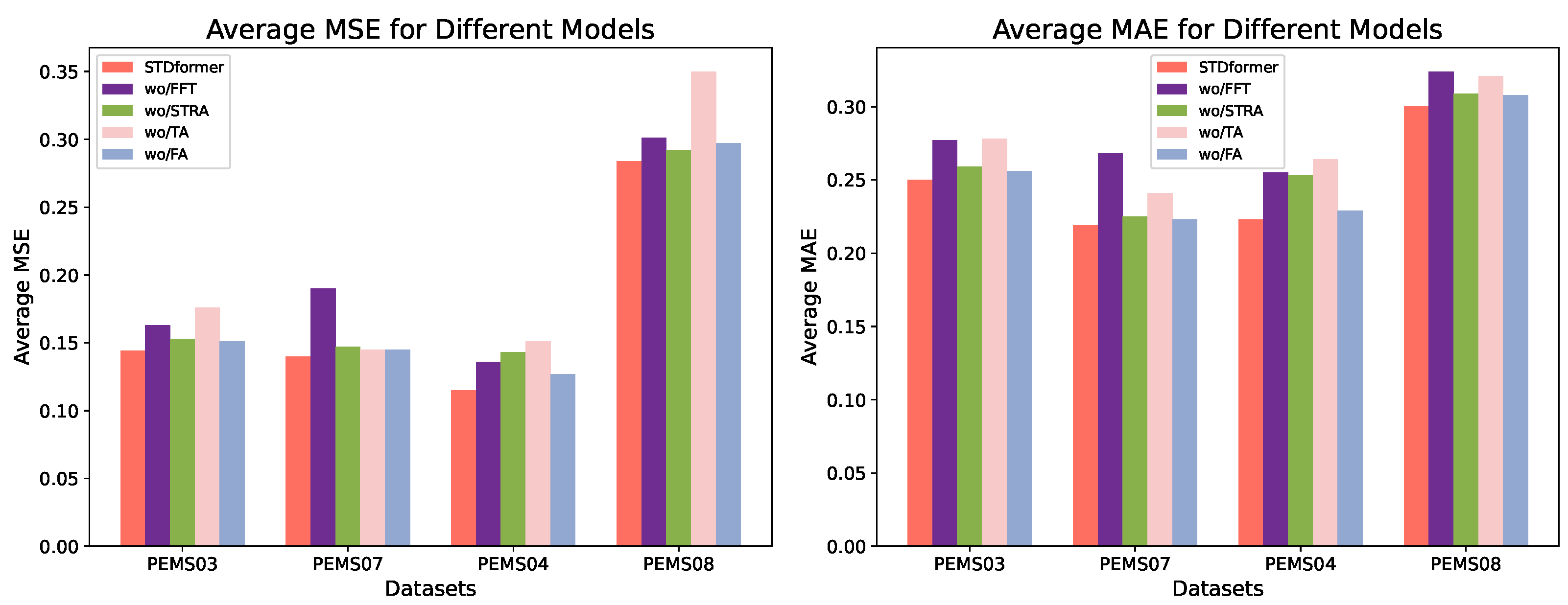
The ablation experiments show substantial performance drops for wo/TA and wo/FA, both of which replace the key modeling mechanisms for the trend and seasonal components with a Multi-Layer Perceptron (MLP). The average MSE and MAE for wo/TA rise to 0.176 and 0.278, respectively, indicating that the Transformer significantly outperforms the MLP in modeling the trend component. Similarly, wo/FA has average MSE and MAE values of 0.148 and 0.253, respectively, highlighting the importance of the Fourier attention mechanism in modeling the seasonal component. These results underscore that the temporal modeling module (trend and seasonal components) in STDformer is key to enhancing model performance, particularly in capturing complex time series patterns, where the combination of Transformer and Fourier attention mechanisms provides significant advantages.

The results of the experiment with wo/STRA indicate that removing the spatial attention module for traffic flow leads to a significant decline in model performance, demonstrating that the spatial correlation of traffic flow speed contributes considerably to the predictive effectiveness of the model.

In the application of more complex traffic conditions, as shown in

Table 8. Ablation study on PEMS04 dataset.

Horizon	STDformer		wo/FFT		wo/STRA		wo/TA		wo/FA
	MSE	MAE	MSE	MAE	MSE	MAE	MSE	MAE	MSE	MAE
12	0.072	0.176	0.109	0.228	0.131	0.241	0.077	0.186	0.072	0.177
24	0.082	0.189	0.115	0.236	0.144	0.251	0.094	0.208	0.083	0.191
48	0.097	0.208	0.125	0.248	0.163	0.270	0.121	0.240	0.098	0.210
96	0.116	0.229	0.131	0.254	0.120	0.232	0.152	0.271	0.117	0.230
192	0.132	0.242	0.144	0.263	0.134	0.254	0.180	0.296	0.134	0.245
336	0.143	0.250	0.155	0.270	0.147	0.256	0.195	0.304	0.146	0.252
720	0.162	0.268	0.171	0.284	0.163	0.269	0.235	0.339	0.168	0.272
Avg	0.115	0.223	0.136	0.255	0.143	0.253	0.151	0.264	0.117	0.225

Note: Optimal MSE and MAE values are marked in bold.

and

Table 9. Ablationstudy on PEMS08 dataset.

Horizon	STDformer		wo/FFT		wo/STRA		wo/TA		wo/FA
	MSE	MAE	MSE	MAE	MSE	MAE	MSE	MAE	MSE	MAE
12	0.188	0.229	0.231	0.268	0.198	0.237	0.195	0.231	0.194	0.234
24	0.217	0.251	0.253	0.286	0.223	0.258	0.276	0.264	0.218	0.260
48	0.236	0.269	0.280	0.311	0.245	0.282	0.278	0.331	0.236	0.270
96	0.275	0.303	0.304	0.339	0.281	0.307	0.347	0.379	0.277	0.304
192	0.319	0.333	0.335	0.361	0.322	0.339	0.416	0.411	0.329	0.348
336	0.360	0.354	0.361	0.367	0.381	0.374	0.428	0.409	0.362	0.359
720	0.393	0.364	0.394	0.364	0.396	0.365	0.467	0.425	0.394	0.368
Avg	0.284	0.300	0.301	0.324	0.292	0.309	0.350	0.321	0.287	0.305

Note: Optimal MSE and MAE values are marked in bold.

. Both wo/TA and wo/FA ablation experiments show significant performance drops. In more complex traffic conditions (e.g., PEMS04), the impact of modeling the trend and seasonal components is far less than that of the spatial component. Conversely, in the simpler traffic conditions with fewer features in the PEMS08 dataset, the modeling impact of the trend and seasonal components is noticeably enhanced. However, the performance declines across both datasets indicate that replacing the Transformer modeling of the trend component with an MLP significantly affects model performance, suggesting that the Transformer outperforms the MLP in trend component modeling. Similarly, the performance drop in wo/FA underscores the importance of the Fourier attention mechanism in modeling the seasonal component.

Overall, the ablation study results for STDformer indicate that, in the short term, modeling the residual component has a significant impact on model accuracy. The combination of the Transformer and Fourier attention mechanisms provides a substantial advantage in capturing complex time series patterns. The gating mechanism of the model ensures that it can dynamically adjust the focus on different components, allowing for flexible responses to various types of traffic fluctuations. The parallel spatiotemporal attention mechanism demonstrates excellent spatial feature-capturing capabilities in complex traffic scenarios.

Figure 4 shows the comparison of these variants on PeMS03, PeMS07, PeMS04, and PeMS08 datasets. From the results, we obtain the following conclusions. In summary, the results of the ablation experiments validate the importance of each component of STDformer in traffic flow prediction. The FFT significantly enhances residual modeling in the short term, while the core modeling mechanisms for trend and seasonal components (Transformer and Fourier attention) effectively capture temporal dependencies. The spatial attention module captures the spatial correlation of traffic flow, which is crucial for achieving high-accuracy predictions. The overall architecture of STDformer effectively integrates temporal and spatial characteristics, providing an optimal solution for traffic flow prediction tasks.

5.3. Parameter Analysis

Finally, we turn to investigate the sensitivity of STDformer. We studied the impact of the number of attention heads on the model’s prediction metrics. Note that while varying one hyperparameter, all other hyperparameters were kept constant. All sensitivity analyses were conducted using the PEMS03 dataset. STDformer-2 represents the number of heads in the multi-head attention mechanism as 2, while STDformer-4 represents the number of heads as 4.

Table 10. Comparison of forecasting performance on the PEMS07 dataset.

Model	STDformer-2		STDformer-4		STDformer-6		STDformer-8
	MSE	MAE	MSE	MAE	MSE	MAE	MSE	MAE
12	0.123	0.234	0.113	0.221	0.094	0.202	0.078	0.183
24	0.148	0.258	0.134	0.239	0.114	0.219	0.096	0.204
48	0.171	0.276	0.158	0.263	0.146	0.250	0.127	0.238
96	0.202	0.316	0.189	0.298	0.174	0.282	0.156	0.269
192	0.215	0.322	0.202	0.308	0.183	0.294	0.168	0.276
336	0.207	0.322	0.195	0.307	0.183	0.288	0.168	0.274
720	0.258	0.352	0.241	0.337	0.228	0.326	0.215	0.310
Avg	0.189	0.297	0.176	0.282	0.160	0.266	0.144	0.250

Note: Optimal MSE and MAE values are marked in bold.

presents the experimental results of the parameter analysis.

The experimental results indicate that the number of attention heads significantly affects model performance; however, increasing the number of heads does not necessarily lead to performance improvements. Based on the experimental findings, the final number of attention heads is set to 8 to achieve a balance between model performance and computational efficiency.

6. Conclusions

This paper presents a novel framework, STDformer, for traffic flow prediction, which is an important and complex task in urban traffic management and planning. Unlike most existing traffic flow prediction studies that primarily focus on either local temporal variations or long-term dependencies, our approach effectively integrates both aspects by decomposing time series data into trend, seasonal, and residual components.

By utilizing gated mechanism fusion for component integration and leveraging spatial attention to model inter-traffic flow dependencies, our approach not only captures intricate temporal dynamics but also effectively accounts for spatial relationships between different traffic flows, leading to superior performance in traffic flow prediction. The modeling of seasonal, trend, and residual components enhances the accuracy of both short-term and long-term modeling of traffic flow data. Furthermore, this decomposition, combined with spatial modeling, allows our model to capture complex and dynamic temporal patterns and spatial dependencies, significantly enhancing forecasting accuracy and robustness. We validated the effectiveness of our model through extensive experiments on the PEMS dataset, demonstrating its performance superiority over state-of-the-art models and highlighting the practical utility of STDformer in real-world traffic management scenarios, assisting urban traffic managers in making informed decisions and optimizing traffic flow.

Although the work presented in this paper performs well in real-world traffic scenarios, it still has some limitations, such as the potential for more flexibility in capturing the spatiotemporal dynamics of the model. Future research could explore integrating large language models or models like Mamba for spatiotemporal dynamic modeling. Additionally, applications such as stock price prediction also exhibit significant periodic characteristics and spatial relationships. For example, fluctuations in chip industry stock prices can affect those in the automotive industry, and stocks tend to show similar patterns of fluctuation each quarter. Therefore, our model has potential application value in stock price prediction.

References

1. Park, C.; Lee, C.; Bahng, H.; Tea, Y.; Jin, S.; Kim, K.; Ko, S.; Choo, J. ST-GRAT: A novel spatio-temporal graph attention networks for accurately forecasting dynamically changing road speed. In Proceedings of the 29th ACM International Conference on Information & Knowledge Management, Virtual, 19–23 October 2020; pp. 1215–1224. [Google Scholar]
2. Lee, C.; Kim, Y.; Jin, S.; Kim, D.; Maciejewski, R.; Ebert, D.; Ko, S. A visual analytics system for exploring, monitoring, and forecasting road traffic congestion. IEEE Trans. Vis. Comput. Graph. 2019, 26, 3133–3146. [Google Scholar] [CrossRef]
3. Lee, H.; Jin, S.; Chu, H.; Lim, H.; Ko, S. Learning to remember patterns: Pattern matching memory networks for traffic forecasting. arXiv 2021, arXiv:2110.10380. [Google Scholar]
4. Lee, H.; Ko, S. TESTAM: A time-enhanced spatio-temporal attention model with mixture of experts. arXiv 2024, arXiv:2403.02600. [Google Scholar]
5. Yu, Q.; Ding, W.; Zhang, H.; Yang, Y.; Zhang, T. Rethinking Attention Mechanism for Spatio-Temporal Modeling: A Decoupling Perspective in Traffic Flow Prediction. In Proceedings of the 33rd ACM International Conference on Information and Knowledge Management, Boise, ID, USA, 21–25 October 2024; pp. 3032–3041. [Google Scholar]
6. Zeng, J.; Qian, Y.; Yin, F.; Zhu, L.; Xu, D. A multi-value cellular automata model for multi-lane traffic flow under Lagrange coordinate. Comput. Math. Organ. Theory 2022, 28, 178–192. [Google Scholar] [CrossRef]
7. Durbin, J.; Koopman, S.J. Time Series Analysis by State Space Methods; Oxford University Press: Oxford, UK, 2012. [Google Scholar]
8. Jiang, D.; Li, Z. Design of a Comprehensive Intelligent Traffic Network Model for Baltimore with Consideration of Multiple Factors. Electronics 2025, 14, 2222. [Google Scholar] [CrossRef]
9. Dubey, A.K.; Kumar, A.; García-Díaz, V.; Sharma, A.K.; Kanhaiya, K. Study and analysis of SARIMA and LSTM in forecasting time series data. Sustain. Energy Technol. Assess. 2021, 47, 101474. [Google Scholar]
10. Zhang, F.; Guo, T.; Wang, H. DFNet: Decomposition fusion model for long sequence time-series forecasting. Knowl.-Based Syst. 2023, 277, 110794. [Google Scholar] [CrossRef]
11. Nidhi, N.; Lobiyal, D.K. Traffic flow prediction using support vector regression. Int. J. Inf. Technol. 2022, 14, 619–626. [Google Scholar] [CrossRef]
12. Kamińska, J.A. The use of random forests in modelling short-term air pollution effects based on traffic and meteorological conditions: A case study in Wrocław. J. Environ. Manag. 2018, 217, 164–174. [Google Scholar] [CrossRef]
13. Han, H.; Zhang, M.; Hou, M.; Zhang, F.; Wang, Z.; Chen, E.; Liu, Q. STGCN: A spatial-temporal aware graph learning method for POI recommendation. In Proceedings of the 2020 IEEE International Conference on Data Mining (ICDM), Sorrento, Italy, 17–20 November 2020; pp. 1052–1057. [Google Scholar]
14. Li, Y.; Yu, R.; Shahabi, C.; Liu, Y. Diffusion convolutional recurrent neural network: Data-driven traffic forecasting. arXiv 2017, arXiv:1707.01926. [Google Scholar]
15. Zhao, Z.; Chen, W.; Wu, X.; Chen, P.C.; Liu, J. LSTM network: A deep learning approach for short-term traffic forecast. IET Intell. Transp. Syst. 2017, 11, 68–75. [Google Scholar] [CrossRef]
16. Zhou, H.; Ren, D.; Xia, H.; Fan, M.; Yang, X.; Huang, H. Ast-gnn: An attention-based spatio-temporal graph neural network for interaction-aware pedestrian trajectory prediction. Neurocomputing 2021, 445, 298–308. [Google Scholar] [CrossRef]
17. He, P.; Shi, Z.; Cui, Y.; Wang, R.; Wu, D. Spatiotemporal Graph Transformer Network Based on Adversarial Training for AD Diagnosis. In Proceedings of the ICC 2023—IEEE International Conference on Communications, Rome, Italy, 28 May–1 June 2023; pp. 3407–3412. [Google Scholar]
18. Cao, J.; Zhu, M.; Wen, Y.; Liu, Y.; Zheng, X. Spatial-Temporal Zero-Inflated Negative Binomial Graph Neural Network-Powered Multi-Port Vessel Traffic Flow Prediction. In Proceedings of the International Conference on Artificial Intelligence and Autonomous Transportation; Springer Nature: Singapore, 2024; pp. 252–260. [Google Scholar]
19. Zhang, J.; Zheng, Y.; Qi, D.; Li, R.; Yi, X. DNN-based prediction model for spatio-temporal data. In Proceedings of the 24th ACM SIGSPATIAL International Conference on Advances in Geographic Information Systems, Burlingame, CA, USA, 31 October–3 November 2016; pp. 1–4. [Google Scholar]
20. Veličković, P.; Cucurull, G.; Casanova, A.; Romero, A.; Lio, P.; Bengio, Y. Graph attention networks. arXiv 2017, arXiv:1710.10903. [Google Scholar]
21. Wu, Z.; Pan, S.; Long, G.; Jiang, J.; Chang, X.; Zhang, C. Connecting the dots: Multivariate time series forecasting with graph neural networks. In Proceedings of the 26th ACM SIGKDD International Conference on Knowledge Discovery & Data Mining, Virtual Event, 6–10 July 2020; pp. 753–763. [Google Scholar]
22. Hwang, D.; Kim, J.J.; Moon, S.; Wang, S. Image Augmentation Approaches for Building Dimension Estimation in Street View Images Using Object Detection and Instance Segmentation Based on Deep Learning. Appl. Sci. 2025, 15, 2525. [Google Scholar] [CrossRef]
23. Cleveland, R.B.; Cleveland, W.S.; McRae, J.E.; Terpenning, I. STL: A seasonal-trend decomposition. J. Off. Stat. 1990, 6, 3–73. [Google Scholar]
24. Wu, H.; Xu, J.; Wang, J.; Long, M. Autoformer: Decomposition transformers with auto-correlation for long-term series forecasting. Adv. Neural Inf. Process. Syst. 2021, 34, 22419–22430. [Google Scholar]
25. Zeng, A.; Chen, M.; Zhang, L.; Xu, Q. Are transformers effective for time series forecasting? In Proceedings of the 37th AAAI Conference on Artificial Intelligence, Washington, DC, USA, 7–14 February 2023; pp. 11121–11128. [Google Scholar] [CrossRef]
26. Zhou, T.; Ma, Z.; Wen, Q.; Wang, X.; Sun, L.; Jin, R. Fedformer: Frequency enhanced decomposed transformer for long-term series forecasting. In Proceedings of the International Conference on Machine Learning, PMLR: 2022, Baltimore, MD, USA, 17–23 July 2022; pp. 27268–27286. [Google Scholar]
27. Wu, H.; Hu, T.; Liu, Y.; Zhou, H.; Wang, J.; Long, M. Timesnet: Temporal 2D-variation modeling for general time series analysis. arXiv 2022, arXiv:2210.02186. [Google Scholar]
28. Oreshkin, B.N.; Carpov, D.; Chapados, N.; Bengio, Y. N-BEATS: Neural basis expansion analysis for interpretable time series forecasting. arXiv 2019, arXiv:1905.10437. [Google Scholar]
29. Challu, C.; Olivares, K.G.; Oreshkin, B.N.; Ramirez, F.G.; Canseco, M.M.; Dubrawski, A. Nhits: Neural hierarchical interpolation for time series forecasting. In Proceedings of the 37th AAAI Conference on Artificial Intelligence, Washington, DC, USA, 7–14 February 2023; pp. 6989–6997. [Google Scholar]
30. Han, J.; Kim, J.; Kim, S.; Wang, S. Effectiveness of image augmentation techniques on detection of building characteristics from street view images using deep learning. J. Constr. Eng. Manag. 2024, 150, 04024129. [Google Scholar] [CrossRef]
31. Cheng, L.; Du, L.; Liu, C.; Hu, Y.; Fang, F.; Ward, T. Multi-modal fusion for business process prediction in call center scenarios. Inf. Fusion 2024, 108, 102362. [Google Scholar] [CrossRef]
32. Tang, L.H.; Bai, Y.L.; Yang, J.; Lu, Y.N. A hybrid prediction method based on empirical mode decomposition and multiple model fusion for chaotic time series. Chaos Solitons Fractals 2020, 141, 110366. [Google Scholar] [CrossRef]
33. Zhang, X.; Jin, X.; Gopalswamy, K.; Gupta, G.; Park, Y.; Shi, X.; Wang, Y. First de-trend then attend: Rethinking attention for time-series forecasting. arXiv 2022, arXiv:2212.08151. [Google Scholar]
34. Dai, T.; Wu, B.; Liu, P.; Li, N.; Bao, J.; Jiang, Y.; Xia, S.T. Periodicity decoupling framework for long-term series forecasting. In Proceedings of the Twelfth International Conference on Learning Representations, Vienna, Austria, 7–11 May 2024. [Google Scholar]
35. Vaswani, A.; Shazeer, N.; Parmar, N.; Uszkoreit, J.; Jones, L.; Gomez, A.N.; Polosukhin, I. Attention is all you need. In Proceedings of the Advances in Neural Information Processing Systems, Long Beach, CA, USA, 4–9 December 2017; Volume 30. [Google Scholar]
36. Lin, S.; Lin, W.; Hu, X.; Wu, W.; Mo, R.; Zhong, H. Cyclenet: Enhancing time series forecasting through modeling periodic patterns. Adv. Neural Inf. Process. Syst. 2024, 37, 106315–106345. [Google Scholar]
37. Liu, Y.; Hu, T.; Zhang, H.; Wu, H.; Wang, S.; Ma, L.; Long, M. itransformer: Inverted transformers are effective for time series forecasting. arXiv 2023, arXiv:2310.06625. [Google Scholar]
38. Nie, Y.; Nguyen, N.H.; Sinthong, P.; Kalagnanam, J. A time series is worth 64 words: Long-term forecasting with transformers. arXiv 2022, arXiv:2211.14730. [Google Scholar]
Figure 1. Framework of the STDformer.
Electronics 14 02400 g001
Figure 2. Framework of the Trend Decomposition Block.
Electronics 14 02400 g002
Figure 3. The framework of Temporal Modeling Block.
Electronics 14 02400 g003
Figure 4. Ablation study on PEMS03, PEMS07, PEMS04, and PEMS08.
Electronics 14 02400 g004