Next Article in Journal
Security and Privacy for Modern Wireless Communication Systems, 2nd Edition
Previous Article in Journal
Real-Time Kubernetes-Based Front-End Processor for Smart Grid
Previous Article in Special Issue
Neural Moving Horizon Estimation: A Systematic Literature Review
 
 
Due to scheduled maintenance work on our database systems, there may be short service disruptions on this website between 10:00 and 11:00 CEST on June 14th.
Article

iTransformer-FFC: A Frequency-Aware Transformer Framework for Multi-Scale Time Series Forecasting

School of Software, Henan Polytechnic University, No. 2001, Century Avenue, Shanyang District, Jiaozuo 454000, China
*
Author to whom correspondence should be addressed.
Electronics 2025, 14(12), 2378; https://doi.org/10.3390/electronics14122378
Submission received: 19 May 2025 / Revised: 8 June 2025 / Accepted: 9 June 2025 / Published: 10 June 2025

Abstract

:
Capturing complex temporal dependencies across multiple scales remains a fundamental challenge in time series forecasting. Transformer-based models have achieved impressive performance on sequence tasks, but vanilla designs often struggle to integrate information from both local fluctuations and global trends, especially in non-stationary sequences. We propose iTransformer-FFC, a novel forecasting framework that addresses these issues through frequency-domain analysis and multi-scale feature fusion. In particular, iTransformer-FFC introduces a Fast Fourier Convolution (FFC) module to transform time series data into the frequency domain, isolating dominant periodic components and attenuating noise before attention is applied. A hierarchical feature fusion mechanism that integrates features extracted at multiple temporal resolutions then jointly models global and local temporal patterns, while a factorized self-attention architecture reduces the quadratic complexity of standard Transformers, improving efficiency while maintaining accuracy. Together, these innovations enable more effective long-range dependency modeling and adaptability to regime shifts in the data. Extensive experiments on five public benchmark datasets demonstrate that iTransformer-FFC consistently outperforms state-of-the-art models, including the vanilla Transformer, an earlier iTransformer variant, and PatchTST. Notably, our model achieves on average an 8.73% lower MSE and 6.95% lower MAE than the best performing baseline, confirming its superior predictive accuracy and generalization in multi-scale time series forecasting through its innovative integration of frequency-domain analysis, hierarchical feature fusion, and factorized attention mechanisms.

1. Introduction

Time series forecasting is crucial in many domains—for example, traffic flow management [1], financial markets [2], and energy systems [3]—yet it remains a challenging task due to the entangled nature of multiple temporal patterns. This complexity poses significant challenges for accurate forecasting, particularly in the presence of shifting patterns and varying temporal dependencies [4,5]. A common approach to handle this complexity is to decompose the time series into a few simpler components, each representing an underlying pattern [6,7]. Traditional statistical methods typically separate a series into trend and seasonal parts and then make predictions based on these components. With the rise of deep learning, some researchers have integrated classical decomposition with neural networks [8,9,10], feeding extracted trend and seasonal signals into deep models. Others have endowed deep learning models with the ability to internally disentangle temporal patterns—using progressive multi-scale decomposition [11], contrastive learning supervision [12], or variational inference techniques [13]—to capture complex temporal dynamics in a more flexible representation.
With the proliferation of high-frequency data across scientific and industrial domains, deep learning has emerged as a principal approach for time series forecasting. Despite the proven effectiveness of deep architectures such as Convolutional Neural Networks (CNNs) and Recurrent Neural Networks (RNNs) in handling spatiotemporal data, and their gated variants have achieved notable success in capturing short-term dependencies and nonlinear dynamics, they remain limited in their ability to model long-range temporal structures, multi-scale interactions, and non-stationary behaviors inherent in real-world sequences [14,15]. These limitations are particularly evident in long-horizon forecasting tasks, where performance often deteriorates due to insufficient temporal context modeling [16].
More recently, Transformer-based architectures have garnered attention for their capacity to capture global dependencies through self-attention mechanisms and their suitability for parallel computation [17]. However, directly transferring the standard Transformer to time series applications reveals several structural inadequacies. Chief among these are the reliance on fixed positional encodings, which fail to incorporate domain-specific temporal priors such as periodicity and seasonality [18], and the uniform treatment of all time steps, which neglects the varying importance of local versus global patterns [19]. Additionally, the quadratic computational complexity of full attention limits the model’s scalability to longer input sequences and increases susceptibility to overfitting under noisy or irregular data regimes [20].
To address these challenges, a model was developed, called iTransformer-FFC, an improved Transformer-based model tailored for multi-scale time series forecasting. A central innovation of iTransformer-FFC is the integration of a Fast Fourier Convolution (FFC) module at the input stage, which transforms raw temporal signals into a frequency-domain representation [21]. Frequency-domain transformation offers a principled way to isolate periodic components and reduce noise, which can enhance the effectiveness of attention mechanisms in capturing relevant temporal features. Integrating frequency-domain processing before the attention mechanism is particularly beneficial because it allows the model to suppress high-frequency noise and emphasize dominant periodic trends at an early stage. This pre-filtering improves the signal-to-noise ratio of the input representation, enabling the self-attention mechanism to operate on a cleaner, more structured signal. As a result, the model is better positioned to capture long-term dependencies and avoid being misled by transient or irrelevant fluctuations, ultimately enhancing both accuracy and generalization [22]. By incorporating spectral information upfront, our approach provides the Transformer with a richer representation of temporal patterns, thereby offering an expressive characterization of both local fluctuations and long-range trends. In essence, the FFC module acts as a feature extractor that emphasizes important cyclical behaviors, complementing the time-domain learning in subsequent layers [23].
The architectural innovations and methodological advancements of iTransformer-FFC are highlighted below:
  • Hierarchical temporal modeling: iTransformer-FFC integrates Inception-style convolution and factorized attention to jointly capture short-term and long-term temporal dependencies with reduced computational cost.
  • Frequency-aware feature enhancement: The model employs Fast Fourier Convolution (FFC) to extract dominant periodic components and suppress high-frequency noise, improving robustness to non-stationarity.
  • Improved long-horizon forecasting: Through multi-scale fusion and efficient attention, the model achieves superior accuracy and stability over extended prediction windows.
To evaluate the effectiveness of the proposed architecture, comprehensive experiments are carried out on five publicly available benchmark datasets spanning diverse time series forecasting tasks. Compared to both classical Transformer variants and recent advanced models such as PatchTST, iTransformer-FFC consistently achieves superior predictive accuracy. These results confirm that the integration of frequency-domain convolution and hierarchical attention mechanisms effectively enhances the Transformer’s capability to model long-range dependencies, handle non-stationarity, and generalize across multiple temporal scales. The remainder of this paper is structured as follows. Section 2 reviews related work; Section 3 presents the proposed iTransformer-FFC model; Section 4 describes the experimental setup; Section 5 discusses the results and outlines future work.

2. Related Work

Time series forecasting has historically employed a variety of statistical and machine learning models, including ARIMA, GARCH, and ETS, which offer interpretable frameworks for capturing linear trends and volatility patterns [24,25,26]. While classical models like ETS exhibit robustness under noisy conditions and have demonstrated utility in short-term, time-sensitive applications such as those reported by Lwin et al. [27], they lack the capacity to model complex nonlinear and multi-scale dependencies. Inspired by such robustness, our work incorporates frequency-domain processing to enhance noise suppression, extending this advantage through a deep learning framework that captures richer temporal structures. These models excel at capturing linear relationships and volatility patterns prevalent in time series data. However, their ability to model complex nonlinear patterns, which are often present in time series, remains limited [28]. Although algorithms such as Support Vector Machines (SVMs) and Random Forests (RFs) have been employed in time series forecasting tasks, their limited capacity to capture sequential dependencies and dynamic temporal structures often constrains their predictive accuracy [29].
Deep learning has brought transformative advancements across diverse application areas due to its strong capability in modeling intricate data structures. Its adoption spans disciplines such as healthcare [30,31,32,33,34], commerce [35], structural engineering [36], behavioral science [37], and financial markets [38]. In the context of stock market prediction, Recurrent Neural Networks (RNNs) have demonstrated notable success by processing temporal sequences via recurrent hidden states. Nonetheless, conventional RNNs are limited in their capacity to capture extended temporal dependencies, often hindered by gradient vanishing or explosion problems [39]. To address these challenges, Long Short-Term Memory (LSTM) networks were introduced [40], incorporating specialized memory units and gating mechanisms that allow the retention and manipulation of long-range information. Empirical evidence suggests that LSTM-based architectures offer superior predictive performance over traditional statistical methods, particularly in capturing short-term fluctuations in financial time series [41,42].
Despite the Transformer model’s extensive adoption and its proven efficacy in numerous sequential modelling tasks, its utilization in time series forecasting remains constrained by several significant limitations. Firstly, the self-attention mechanism of the Transformer exhibits quadratic computational complexity with respect to sequence length [43]. This results in substantial computational resource consumption and reduced scalability when processing long sequences. Secondly, the fixed positional encoding employed by the traditional Transformer is inadequate in effectively representing the periodic patterns that are commonly observed in time series data [44]. This limitation restricts the model’s capacity to capture complex temporal dependencies. Furthermore, the global attention mechanism increases the risk of overfitting when applied to noisy datasets, which are characteristic of real-world markets, ultimately impairing the model’s generalization performance [45]. Consequently, there is a necessity to develop structural optimizations and methodological enhancements to address the shortcomings of the Transformer in terms of computational efficiency, temporal modelling capabilities, and robustness against noise, thereby improving its applicability to time series forecasting tasks [46].

3. Methodology

3.1. Problem Formulation

In this work, we addressed the challenge of forecasting multivariate time series, which involves predicting future values across multiple interdependent variables over time. More formally, given a series of fully observed time series signals Y = y 1 , y 2 , , y T , w h e r e y t R n and n is the variable dimension, we aimed to predict a series of future signals in a rolling forecasting fashion. Specifically, to predict y T + h , where h is the desirable horizon ahead of the current time stamp, we assumed { y 1 , y 2 , , y T } are available. Likewise, to predict the value of the next time stamp y T + h + 1 , we assumed { y 1 , y 2 , , y T , y T + 1 } are available. We hence formulated the input matrix at time stamp T as X T = { y 1 , y 2 , , y T } R n × T .

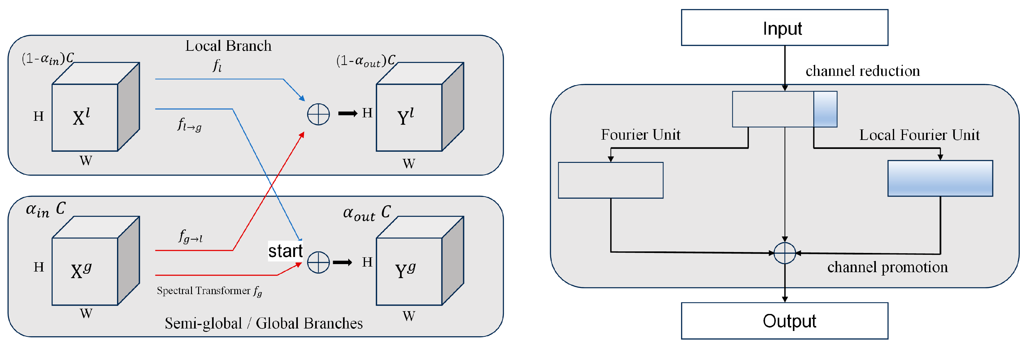
3.2. Fast Fourier Convolution (FFC)

3.2.1. FFC Architectural Design

The architecture of our proposed FFC module for sequence prediction is illustrated in Figure 1. Conceptually, FFC consists of two interconnected branches: a local path, which applies standard 1D convolutions to capture short-range dependencies, and a global path, which performs operations in the frequency domain to model long-range dependencies in the sequence.
Formally, let X R L × C be the input feature sequence, where L denotes the sequence length and C the number of channels. At the entry of FFC, we split the input along the channel dimension into a local part X l R L × ( 1 α i n ) C and a global part X g R L × α i n C , where α i n [ 0,1 ] controls the proportion of channels assigned to the global path.
The local path processes X l using standard 1D convolutional layers to extract features from the local context, while the global path transforms X g to the frequency domain using the Fast Fourier Transform (FFT), applies learnable filters, and then transforms it back using the inverse FFT to capture global trends. The output tensor is denoted by Y R L × C , which is also split into Y l and Y g following a predefined output ratio α o u t [ 0,1 ] . The final output is obtained by concatenating Y l and Y g along the channel dimension. Internal fusion mechanisms allow information exchange between the two branches, enhancing the network’s capacity to model both local dynamics and global temporal dependencies. This preprocessing allows the attention module to operate on more structured, noise-reduced signals, enhancing long-range pattern recognition.
Y l = f l X l + f g l X g
Y g = f g X g + f l g X l
where f l ( X l ) captures local patterns via standard 1D convolution, while f g ( X g ) , implemented as a spectral transformer, models long-range dependencies in the frequency domain. The cross-path terms f g l ( X g ) and f l g ( X l ) enable bidirectional information exchange between local and global branches, enhancing feature representation. For statement clarity, we termed f g as a spectral transformer.

3.2.2. Spectral Transformer
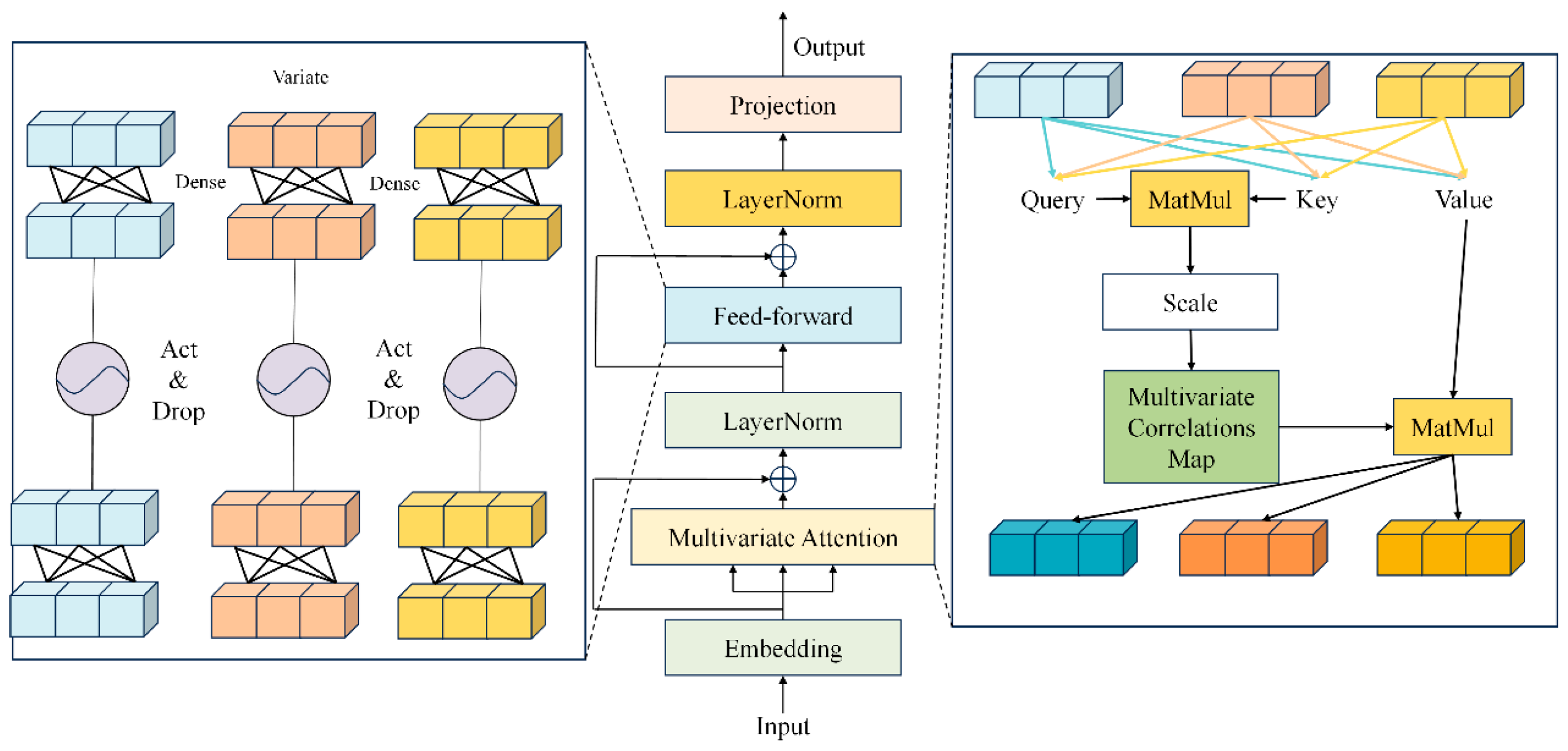
The objective of the global path in Figure 1 is to efficiently expand the receptive field of convolutions, enabling the model to capture long-range dependencies across the entire sequence. To achieve this, we adopted the Discrete Fourier Transform (DFT), leveraging the accelerated Cooley–Tukey algorithm. As depicted in Figure 1, our spectral transformer was inspired by the bottleneck block in ResNet. To reduce computational complexity, we began with a 1 × 1 convolution that reduces the number of channels, followed by another 1 × 1 convolution to restore the feature channel dimension. Between these two convolutions, we introduced a Fourier Unit (FU) to capture global temporal patterns, a Local Fourier Unit (LFU) that operates on a subset of feature channels to capture semi-global dependencies, and a residual connection to improve model stability and facilitate efficient information flow. The details of the FU and LFU are discussed below.

3.3. Itransformer

The iTransformer is an improved neural architecture derived from the Transformer model. Unlike the standard Transformer, it encodes separate time series as individual tokens, allowing the model to capture inter-series dependencies via self-attention mechanisms. It further integrates layer normalization and feed-forward networks to enhance global feature extraction for forecasting tasks. These enhancements improve the model’s adaptability and performance, especially in long-sequence scenarios. Figure 2 presents the detailed architecture of iTransformer, which includes the following main components:
Embedding: The input variates are mapped to generate embedded tokens of dimension D. Positional encoding is used to inject information about the relative position of the sequences. The embedded token of dimension D for feature n is expressed by:
h n 0 = E m b e d d i n g X : , n
Multivariate Attention: This layer captures the dependencies between features by applying the self-attention mechanism on each variate time series. Given the representation of each time series H 1 = { h 1 , , h N } at the l t h layer, the queries, keys, and values Q , K , and V are generated through linear projections.
A t t e n t i o n Q , K , V = s o f t m a x Q K T d k V
h e a d i = A t t e n t i o n H l 1 W Q l , H l 1 W K l , H l 1 W V l
M u l t i H e a d H l 1 = h e a d 1 ; ; h e a d h W O
where W Q l , W Q l and W Q l R D × d k are projection weights.
Feed-forward Network (FFN): The network encodes the sequential representation of each variate token and employs nonlinear fully connected layers to capture intricate dependencies within the input sequence. Each token is independently processed through the feed-forward network ( F F N ) in a parallel manner
H l = F F N M u l t i H e a d H l 1
Projection: A fully connected layer maps the output from the feed-forward network to obtain the predicted capacity at the next time step.
Y ^ : , n = P r o j e c t i o n h n L

3.4. Model Architecture of iTransformer-FFC

The iTransformer-FFC (Frequency-aware Fully Convolutional iTransformer) is a novel model tailored for multivariate time series forecasting, integrating frequency-domain modeling with fully convolutional representations. Building upon the standard iTransformer framework, this architecture is specifically designed to enhance the representation of periodicity, trends, and abrupt changes, while significantly reducing the computational burden commonly associated with long-sequence modeling in conventional Transformer-based models.
A core innovation of iTransformer-FFC lies in its abandonment of positional encoding, which is traditionally required to encode temporal information. Instead, the model leverages data-driven temporal feature representations and frequency-aware components to address the inherent non-stationarity and multi-scale characteristics of real-world time series. The architecture adopts a two-stage modeling approach comprising an encoder and a decoder. The encoder incorporates a stack of TimesBlocks, each of which is built upon lightweight Factorized Attention and Inception-style Convolution to effectively extract temporal patterns across multiple resolutions and frequency bands. In the decoding phase, a label-length-aware masked decoder is employed to preserve causal dependencies and facilitate autoregressive forecasting. Furthermore, to enhance modeling flexibility across variables, iTransformer-FFC supports both channel-independent and channel-mixing modes. The former performs separate modeling per variable, suitable for loosely coupled dimensions, whereas the latter utilizes attention mechanisms to capture inter-series dependencies, enabling the learning of complex interactions among correlated time series.
To mitigate the long-range dependency degradation inherent in traditional Transformers, iTransformer-FFC integrates a frequency-aware architectural design. Specifically, the TimesBlock module introduces an Inception-style multi-kernel convolution mechanism, allowing the model to represent periodic components of varying scales in the frequency domain. Unlike explicit Fourier transform methods, this design provides a learnable approximation of spectral responses, thereby improving the model’s ability to recognize long-term cycles while maintaining adaptability to non-stationary behavior.
Additionally, a Distillation Module is embedded within the encoder to compress intermediate representations through progressive sequence length reduction. This mechanism enables the preservation of salient features while reducing computational redundancy, thus improving both efficiency and generalization. From an optimization perspective, iTransformer-FFC is trained using the Mean Squared Error (MSE) loss and leverages adaptive learning rate schedules such as Reduce Learning Rate On Plateau to ensure stable convergence and robustness across different time series scenarios.
In summary, iTransformer-FFC provides a comprehensive balance between representational capacity and computational efficiency. It is particularly well-suited for high-dimensional, nonlinear, and hybrid-pattern time series forecasting tasks, where the simultaneous presence of trend, seasonality, and noise poses significant modeling challenges.
The overall model architecture is illustrated in Figure 3, highlighting the interaction between the encoder–decoder structure and the frequency-aware components.

4. Experiments

4.1. Data

To assess the effectiveness of the proposed iTransformer, empirical evaluations were conducted using five real-world benchmark datasets. (1) The ETT dataset comprises seven electrical transformer indicators measured between July 2016 and July 2018. It is divided into four subsets: ETTh1 and ETTh2 with hourly sampling, and ETTm1 and ETTm2 sampled at 15-min intervals. (2) The Exchange dataset consists of daily foreign exchange rate time series from eight different countries, spanning the years from 1990 to 2016. The basic characteristics of these datasets are summarized in Table 1.
These datasets collectively exhibit diverse temporal characteristics such as trend, seasonality, irregular fluctuations, and volatility, allowing for a comprehensive evaluation of model robustness across different dynamic patterns. We employed a set of classical statistical methods to quantify these properties, and a summary of their statistical characteristics is provided in Table 2.

4.2. Evaluation Criteria

Regression model evaluation metrics are essential for quantitatively assessing the predictive accuracy and overall effectiveness of a model in capturing the underlying relationship between input features and output responses.
The Mean Squared Error ( M S E ) quantifies the average squared deviation between predicted and actual values, serving as a fundamental metric for evaluating the predictive accuracy of regression models. A lower M S E indicates a closer fit between the model’s output and the observed data, reflecting superior forecasting performance.
M S E = 1 n i n ( y i y ^ i ) 2 ,
The Mean Absolute Error ( M A E ) evaluates the average magnitude of errors between predicted and actual values by computing the mean of their absolute differences. It serves as a robust and interpretable metric for assessing model accuracy, with lower M A E values indicating better predictive performance.
M A E = 1 n 1 n y i y ^ i ,
The Coefficient of Determination ( R 2 ) serves as a statistical metric to assess the explanatory power of a regression model. It is defined as one minus the ratio of the residual sum of squares (RSS) to the total sum of squares (TSS), thereby quantifying the proportion of variance in the dependent variable that is predictable from the independent variables. An R2 value closer to 1 signifies superior model fidelity and predictive effectiveness
R 2 = 1 y i y ^ i 2 y i y ¯ 2 ,

4.3. Results

This study presents a systematic and comprehensive evaluation of several state-of-the-art time series forecasting algorithms—namely, Transformer, iTransformer, and PatchTST—across five publicly available benchmark datasets. The primary objective is to identify the most effective model in terms of predictive accuracy and computational efficiency for the task of stock price forecasting. Performance is assessed using a set of widely accepted regression evaluation metrics, including Mean Squared Error (MSE), Mean Absolute Error (MAE), and the Coefficient of Determination (R2), to provide a multifaceted measure of model accuracy and generalization capability.
The proposed iTransformer-FFC model demonstrates superior forecasting performance. As depicted in Figure 4, Figure 5, Figure 6 and Figure 7, the blue curves represent the actual stock prices, while the red curves indicate the corresponding predicted values. The close alignment between these curves underscores the model’s ability to accurately capture temporal dynamics. For comparison, Figure 4, Figure 5, Figure 6 and Figure 7 illustrate the forecasting results of iTransformer-FFC, iTransformer, Transformer, and PatchTST, respectively.
To ensure consistency across experiments, we adopted a unified set of training hyperparameters for all models. These settings are summarized in Table 3, including batch size, prediction length, learning rate, and model dimension.
A comparative analysis of MSE values across the evaluated models is presented in Table 4, with the results organized by ticker symbol and model architecture. As a general rule, lower MSE values reflect improved predictive precision. According to the results shown in Figure 8, the iTransformer-FFC consistently achieves the lowest MSE scores on the majority of datasets, suggesting that it is particularly well-suited for complex time series forecasting tasks involving stock price dynamics. Furthermore, Table 4 also reports the Mean Absolute Error (MAE) for each model. As a robust indicator of predictive performance, MAE quantifies the average magnitude of forecast errors. The iTransformer-FFC model records the lowest MAE values among all evaluated models, reinforcing its status as the most accurate predictive model in this comparative study.
On the ETTh1 dataset, iTransformer-FFC achieves an MSE of 0.455, compared to 0.569 for Transformer and 0.633 for PatchTST. Similar trends are observed on the ETTh2 dataset, where iTransformer-FFC obtains an MSE of 0.782, while Transformer and PatchTST yield 2.280 and 2.310, respectively. These results reflect consistent improvements across both moderate and volatile series. The comparison of MAE and MSE across the four benchmark datasets is visualized in Figure 4, clearly illustrating the performance differences of each model under varying temporal volatility and sequence complexity.
The forecasting results presented in this figure demonstrate high accuracy across a wide range of temporal patterns and volatility conditions. The predicted values align closely with the actual observations in upward and downward trends, periodic segments, and regions with intense fluctuations. This performance underscores the model’s strong capacity to capture frequency-dependent characteristics and leverage structural dependencies among time series components, resulting in stable and precise forecasting outcomes across diverse scenarios.
The model depicted in this figure demonstrates generally good alignment with the observed values across most time steps, particularly in stable trend intervals. However, noticeable discrepancies arise in segments characterized by abrupt fluctuations or high-frequency noise. These deviations suggest that the model lacks the capacity to effectively capture complex local dynamics and rapid structural changes within the time series.
This model exhibits improved performance in modeling low-frequency trends, showing enhanced overall fit compared to the previous one. Nonetheless, its predictive accuracy diminishes during intervals of rapid variation, often resulting in lagging forecasts. This indicates limitations in handling non-stationary temporal dependencies and short-term variability.
The results shown in this figure reflect a better response to high-frequency components, as the model captures finer fluctuations with greater sensitivity. However, certain peak and trough points are still missed or inaccurately predicted, reflecting instability in localized patterns. This may stem from insufficient frequency-domain separation or overfitting to periodic signals.

4.4. Experimental Analysis

The comprehensive empirical evaluation across five widely used benchmark datasets—Exchange, ETTh1, ETTh2, ETTm1, and ETTm2—demonstrates that the proposed iTransformer-FFC model consistently outperforms state-of-the-art baseline methods, including Transformer, iTransformer, and PatchTST. The evaluation, conducted under standardized experimental settings, utilizes Mean Absolute Error (MAE), Mean Squared Error (MSE), and the Coefficient of Determination (R2) as primary performance metrics, providing a robust measure of both predictive accuracy and model generalization.
On high-resolution datasets such as ETTm1 and ETTm2, iTransformer-FFC achieves superior performance, with MSE values of 0.114 and 0.078, respectively, and R2 values exceeding 0.99. These results validate the model’s ability to effectively capture intricate temporal dependencies and fine-grained seasonal structures that are often present in dense time series. The model’s use of frequency-aware convolution and factorized attention appears to enhance its sensitivity to periodic patterns while mitigating the effects of short-term noise.
In scenarios involving irregular or volatile patterns—such as those exhibited in the ETTh2 and Exchange datasets—iTransformer-FFC continues to demonstrate its robustness. Compared to the Transformer and iTransformer baselines, the proposed model achieves consistently lower prediction errors and higher R2 scores, highlighting its capacity to adapt to non-stationary dynamics and abrupt regime shifts. This robustness can be attributed to two critical architectural components: (1) the Fast Fourier Convolution (FFC) module, which enables frequency-domain feature learning, and (2) the distillation-based sequence compression mechanism, which reduces temporal redundancy and facilitates more stable training.
In addition, the model’s hybrid design—supporting both channel-independent and channel-mixing pathways—offers flexibility in capturing multivariate dependencies, enabling it to scale effectively across different data granularities and variable correlation structures. The consistently low standard deviations observed across repeated trials further attest to the stability and reliability of the model under various temporal regimes.
In summary, the experimental results substantiate the superiority of iTransformer-FFC in terms of both predictive precision and robustness. Its architectural innovations allow it to model complex, nonlinear, and multi-scale temporal phenomena more effectively than conventional approaches, making it particularly well-suited for real-world time series forecasting applications where accuracy, adaptability, and efficiency are all critical.

4.4.1. Architectural Design

To quantitatively evaluate the individual contribution of each core component in the proposed iTransformer-FFC architecture, we conducted an ablation analysis. Three reduced variants were designed by systematically removing or modifying key modules: (1) removing the Fast Fourier Convolution (FFC) module; (2) replacing the Factorized Self-Attention (FSA) with standard full self-attention; and (3) disabling the hierarchical multi-scale fusion mechanism (MSF) by applying single-scale convolutions only. Experiments were conducted on the ETTm1 and ETTh1 datasets, and the results are presented in Table 5. The complete model consistently achieves the best performance across all metrics, while the exclusion of the FFC module leads to the most significant degradation. These results underscore the importance of frequency-domain representation and multi-scale learning in capturing complex temporal patterns. The detailed results are shown in Table 5.

4.4.2. Robustness and Statistical Significance Analysis

To ensure the robustness of the observed performance improvements, we conducted paired t-tests between the proposed iTransformer-FFC model and each baseline model (iTransformer and PatchTST) under multiple random seed initializations. The null hypothesis assumes no statistically significant difference in forecasting accuracy between the compared models.
The results are summarized in Table 6, which presents the mean differences in MAE, corresponding t-values, p-values, and statistical significance levels for each pairwise comparison. As shown in the table, iTransformer-FFC consistently outperforms both baselines, with p-values < 0.01, indicating that the performance improvements are statistically significant and unlikely to have occurred by chance.

4.4.3. Training and Inference Efficiency

To rigorously evaluate the computational efficiency of iTransformer-FFC in both training and inference, we conducted comparative experiments against the baseline iTransformer using the ETTm1 dataset. All experiments were implemented under identical experimental settings, with consistent data loaders and hyperparameter configurations to ensure methodological fairness. As illustrated in Figure 9, iTransformer-FFC consistently outperforms iTransformer in inference speed across all tested iteration scales. Notably, at 600 iterations, iTransformer-FFC achieves an inference time of 1.11 s, significantly outperforming iTransformer’s 1.90 s, corresponding to a performance gain exceeding 40%. Furthermore, the observed efficiency gap widens progressively with increasing iteration counts, underscoring the superior scalability and computational robustness of the proposed architecture under heavier workloads. All evaluations were executed on the same hardware and software platform, utilizing a single NVIDIA RTX 4090 GPU, to guarantee result reproducibility and eliminate environmental variability.

5. Conclusions

Time series forecasting plays a critical role in a wide range of real-world applications, such as energy systems, industrial monitoring, and environmental analysis. In this work, we propose iTransformer-FFC, a novel forecasting model that enhances traditional Transformer-based architectures with feature fusion components to better capture multi-scale temporal dependencies. We conduct comprehensive experiments on five publicly available benchmark datasets and compare our model against several state-of-the-art baselines, including Transformer, iTransformer, and PatchTST. The evaluation results based on the MSE, MAE, and R2 metrics demonstrate that iTransformerFFC consistently achieves superior performance, confirming its effectiveness in modeling complex temporal dynamics and improving predictive accuracy.
In future work, the model will be extended in two directions. First, we will explore more adaptive and dynamic fusion strategies to improve the model’s generalization to diverse time series characteristics. Second, we aim to enhance the interpretability of the model by incorporating explainable mechanisms, making it more applicable to high-stakes decision-making tasks in real-world scenarios.

Author Contributions

Conceptualization, Y.T. and Z.C.; Methodology, Y.T.; Software, Y.T.; Validation, Y.T. and Z.C.; Formal analysis, Y.T.; Investigation, Y.T.; Resources, Y.T.; Data curation, Y.T.; Writing—original draft preparation, Y.T.; Writing—review and editing, Y.T. and Z.C.; Visualization, Y.T.; Supervision, Z.C.; Project administration, Z.C. All authors have read and agreed to the published version of the manuscript.

Funding

This research was supported in part by the National Natural Science Foundation of China (Project No. 62472144) under the General Program, titled “Research on privacy preserving techniques for blockchain based on non-interactive zero-knowledge proof from lattice”, covering the period from January 2025 to December 2028. Additional support was provided by the Key Scientific and Technological Research Project of Henan Province (Project No. 252102210100). The authors gratefully acknowledge the financial support from both foundations.

Institutional Review Board Statement

Not applicable.

Informed Consent Statement

Not applicable.

Data Availability Statement

Data are contained within the article. The data presented in this study can be requested from the authors.

Conflicts of Interest

The authors declare no conflicts of interest.

References

  1. Lv, Y.; Duan, Y.; Kang, W.; Li, Z.; Wang, F.-Y. Traffic flow prediction with big data: A deep learning approach. IEEE Trans. Intell. Transp. Syst. 2014, 16, 865–873. [Google Scholar] [CrossRef]
  2. Nelson, D.M.Q.; Pereira, A.C.M.; De Oliveira, R.A. Stock market’s price movement prediction with LSTM neural networks. In Proceedings of the2017 International Joint Conference on Neural Networks (IJCNN), Anchorage, AK, USA, 14–19 May 2017; IEEE: Piscataway, NJ, USA, 2017; pp. 1419–1426. [Google Scholar]
  3. Kong, W.; Dong, Z.Y.; Jia, Y.; Hill, D.J.; Xu, Y.; Zhang, Y. Short-term residential load forecasting based on LSTM recurrent neural network. IEEE Trans. Smart Grid 2017, 10, 841–851. [Google Scholar] [CrossRef]
  4. Hyndman, R.J.; Athanasopoulos, G. Forecasting: Principles and Practice; OTexts: Melbourne, Australia, 2018. [Google Scholar]
  5. Zhang, G.; Patuwo, B.E.; Hu, M.Y. Forecasting with artificial neural networks: The state of the art. Int. J. Forecast. 1998, 14, 35–62. [Google Scholar] [CrossRef]
  6. Cleveland, R.B.; Cleveland, W.S.; McRae, J.E.; Terpenning, I. STL: A seasonal-trend decomposition. J. Off. Stat. 1990, 6, 3–73. [Google Scholar]
  7. Hamilton, J.D. A new approach to the economic analysis of nonstationary time series and the business cycle. Econometrica J. Econom. Soc. 1989, 57, 357–384. [Google Scholar] [CrossRef]
  8. Laptev, N.; Yosinski, J.; Li, L.E.; Smyl, S. Time-series extreme event forecasting with neural networks at Uber. In Proceedings of the 34th International Conference on Machine Learning (ICML), Sydney, Australia, 6–11 August 2017; PMLR: Sydney, Australia, 2017; pp. 1–5. [Google Scholar]
  9. Borovykh, A.; Bohte, S.; Oosterlee, C.W. Conditional time series forecasting with convolutional neural networks. arXiv 2017, arXiv:1703.04691. [Google Scholar]
  10. Wen, R.; Torkkola, K.; Narayanaswamy, B.; Madeka, D. A multi-horizon quantile recurrent forecaster. arXiv 2017, arXiv:1711.11053. [Google Scholar]
  11. Wu, H.; Xu, J.; Wang, J.; Long, M. Autoformer: Decomposition transformers with auto-correlation for long-term series forecasting. Adv. Neural Inf. Process. Syst. 2021, 34, 22419–22430. [Google Scholar]
  12. Tonekaboni, S.; Eytan, D.; Goldenberg, A. Unsupervised representation learning for time series with temporal neighborhood coding. arXiv 2021, arXiv:2106.00750. [Google Scholar]
  13. Fortuin, V.; Hüser, M.; Locatello, F.; Strathmann, H.; Rätsch, G. Som-vae: Interpretable discrete representation learning on time series. arXiv 2018, arXiv:1806.02199. [Google Scholar]
  14. Bai, S.; Kolter, J.Z.; Koltun, V. An empirical evaluation of generic convolutional and recurrent networks for sequence modeling. arXiv 2018, arXiv:1803.01271. [Google Scholar]
  15. Lim, B.; Arık, S.Ö.; Loeff, N.; Pfister, T. Temporal fusion transformers for interpretable multi-horizon time series forecasting. Int. J. Forecast. 2021, 37, 1748–1764. [Google Scholar] [CrossRef]
  16. Alharthi, M.; Mahmood, A. xlstmtime: Long-term time series forecasting with xlstm. AI 2024, 5, 1482–1495. [Google Scholar] [CrossRef]
  17. Vaswani, A.; Shazeer, N.; Parmar, N.; Uszkoreit, J.; Jones, L.; Gomez, A.N.; Kaiser, Ł.; Polosukhin, I. Attention is All You Need. Adv. Neural Inf. Process. Syst. (NeurIPS) 2017, 30, 5998–6008. [Google Scholar]
  18. Li, S.; Jin, X.; Xuan, Y.; Zhou, X.; Chen, W.; Wang, Y.X.; Yan, X. Enhancing the locality and breaking the memory bottleneck of transformer on time series forecasting. Adv. Neural Inf. Process. Syst. 2019, 32. [Google Scholar]
  19. Zhou, H.; Zhang, S.; Peng, J.; Zhang, S.; Li, J.; Xiong, H.; Zhang, W. Informer: Beyond Efficient Transformer for Long Sequence Time-Series Forecasting. Proc. AAAI Conf. Artif. Intell. 2021, 35, 11106–11115. [Google Scholar] [CrossRef]
  20. Choromanski, K.; Likhosherstov, V.; Dohan, D.; Song, X.; Gane, A.; Sarlos, T.; Hawkins, P.; Davis, J.; Mohiuddin, A.; Kaiser, L.; et al. Rethinking attention with performers. arXiv 2020, arXiv:2009.14794. [Google Scholar]
  21. Yi, K.; Zhang, Q.; Cao, L.; Wang, S.; Long, G.; Hu, L.; He, H.; Niu, Z.; Fan, W.; Xiong, H. A survey on deep learning based time series analysis with frequency transformation. arXiv 2023, arXiv:2302.02173. [Google Scholar]
  22. Kang, B.G.; Lee, D.; Kim, H.; Chung, D.; Yoon, S. Introducing Spectral Attention for Long-Range Dependency in Time Series Forecasting. arXiv 2024, arXiv:2410.20772. [Google Scholar]
  23. Wu, M.; Gao, Z.; Huang, Y.; Xiao, Z.; Ng, D.W.K.; Zhang, Z. Deep learning-based rate-splitting multiple access for reconfigurable intelligent surface-aided tera-hertz massive MIMO. IEEE J. Sel. Areas Commun. 2023, 41, 1431–1451. [Google Scholar] [CrossRef]
  24. Box, G.E.P.; Jenkins, G.M.; Reinsel, G.C.; Ljung, G.M. Time Series Analysis: Forecasting and Control, 5th ed.; John Wiley & Sons: Hoboken, NJ, USA, 2015. [Google Scholar]
  25. Bollerslev, T. Generalized autoregressive conditional heteroskedasticity. J. Econom. 1986, 31, 307–327. [Google Scholar] [CrossRef]
  26. Hyndman, R.J.; Athanasopoulos, G. Forecasting with Exponential Smoothing: The State Space Approach; Springer Science & Business Media: Berlin/Heidelberg, Germany, 2008. [Google Scholar]
  27. Lwin, T.C.; Zin, T.T.; Tin, P. Predicting Calving Time of Dairy Cows by Exponential Smoothing Models. In Proceedings of the 2020 IEEE 9th Global Conference on Consumer Electronics (GCCE), Kobe, Japan, 13–16 October 2020; IEEE: Piscataway, NJ, USA, 2020. [Google Scholar]
  28. Zhang, G.P. Time series forecasting using a hybrid ARIMA and neural network model. Neurocomputing 2003, 50, 159–175. [Google Scholar] [CrossRef]
  29. Ajiga, D.I.; Adeleye, R.A.; Tubokirifuruar, T.S.; Bello, B.G.; Ndubuisi, N.L.; Asuzu, O.F.; Owolabi, O.R. Machine learning for stock market forecasting: A review of models and accuracy. Financ. Account. Res. J. 2024, 6, 112–124. [Google Scholar]
  30. Miotto, R.; Wang, F.; Wang, S.; Jiang, X.; Dudley, J.T. Deep learning for healthcare: Review, opportunities and challenges. Brief. Bioinform. 2018, 19, 1236–1246. [Google Scholar] [CrossRef]
  31. Esteva, A.; Robicquet, A.; Ramsundar, B.; Kuleshov, V.; DePristo, M.; Chou, K.; Cui, C.; Corrado, G.; Thrun, S.; Dean, J. A guide to deep learning in healthcare. Nat. Med. 2019, 25, 24–29. [Google Scholar] [CrossRef]
  32. Choi, E.; Bahadori, M.T.; Schuetz, A.; Stewart, W.F.; Sun, J. Doctor AI: Predicting Clinical Events via Recurrent Neural Networks. In Proceedings of the Machine Learning for Healthcare Conference (MLHC), PMLR, Los Angeles, CA, USA, 19–20 August 2016; Volume 56, pp. 301–318. [Google Scholar]
  33. Rajkomar, A.; Dean, J.; Kohane, I. Machine learning in medicine. New Engl. J. Med. 2019, 380, 1347–1358. [Google Scholar] [CrossRef]
  34. Razzak, M.I.; Imran, M.; Xu, G. Big data analytics for preventive medicine. Neural Comput. Appl. 2020, 32, 4417–4451. [Google Scholar] [CrossRef]
  35. Darapaneni, N.; Paduri, A.R.; Sharma, H.; Manjrekar, M.; Hindlekar, N.; Bhagat, P.; Aiyer, U.; Agarwal, Y. Stock price prediction using sentiment analysis and deep learning for Indian markets. arXiv 2022, arXiv:2204.05783. [Google Scholar]
  36. Goh, A.T.C. Modeling soil correlations using neural networks. J. Comput. Civ. Eng. 1995, 9, 275–278. [Google Scholar] [CrossRef]
  37. Schmidhuber, J. Deep learning in neural networks: An overview. Neural Netw. 2015, 61, 85–117. [Google Scholar] [CrossRef]
  38. Fischer, T.; Krauss, C. Deep learning with long short-term memory networks for financial market predictions. Eur. J. Oper. Res. 2018, 270, 654–669. [Google Scholar] [CrossRef]
  39. Pascanu, R.; Mikolov, T.; Bengio, Y. On the difficulty of training recurrent neural networks. In Proceedings of the International Conference on Machine Learning, Pmlr, Atlanta, GA, USA, 16–21 June 2013. [Google Scholar]
  40. Sepp, H.; Schmidhuber, J. Long short-term memory. Neural Comput. 1997, 9, 1735–1780. [Google Scholar]
  41. Bao, W.; Yue, J.; Rao, Y. A deep learning framework for financial time series using stacked autoencoders and long-short term memory. PLoS ONE 2017, 12, e0180944. [Google Scholar] [CrossRef] [PubMed]
  42. Kai, C.; Zhou, Y.; Dai, F. An LSTM-Based Method for Stock Returns Prediction: A Case Study of the China Stock Market. In Proceedings of the 2015 IEEE International Conference on Big Data (Big Data), Santa Clara, CA, USA, 29 October–1 November 2015; IEEE: Piscataway, NJ, USA, 2015; pp. 2823–2830. [Google Scholar]
  43. Tay, Y.; Dehghani, M.; Bahri, D.; Metzler, D. Efficient transformers: A survey. ACM Comput. Surv. 2022, 55, 1–28. [Google Scholar] [CrossRef]
  44. Xinhe, L.; Wang, W. Deep time series forecasting models: A comprehensive survey. Mathematics 2024, 12, 1504. [Google Scholar] [CrossRef]
  45. Wu, Z.; Pan, S.; Chen, F.; Long, G.; Zhang, C.; Yu, P.S. A comprehensive survey on graph neural networks. IEEE Trans. Neural Netw. Learn. Syst. 2020, 32, 4–24. [Google Scholar] [CrossRef]
  46. Zeng, A.; Chen, M.; Zhang, L.; Xu, Q. Are transformers effective for time series forecasting? In Proceedings of the AAAI Conference on Artificial Intelligence, Washington, DC, USA, 7–14 February 2023. [Google Scholar]
Figure 1. (Left) Architecture design of Fast Fourier Convolution (FFC).   denotes element-wise sum. Here α i n = α o u t = 0.5 . (Right) Design of spectral transform f g . See main text for further explanations.
Electronics 14 02378 g001
Figure 2. Model architecture of iTransformer.
Electronics 14 02378 g002
Figure 3. The architecture of iTransformer-FFC, a frequency-aware and channel-mixing encoder-decoder framework for time series forecasting.
Electronics 14 02378 g003
Figure 4. iTransformer—FFC results.
Electronics 14 02378 g004
Figure 5. iTransformer results.
Electronics 14 02378 g005
Figure 6. Transformer results.
Electronics 14 02378 g006
Figure 7. PatchTST results.
Electronics 14 02378 g007
Figure 8. Comparison of MSE performance across four datasets for different models.
Electronics 14 02378 g008
Figure 9. Comparison of training and inference times: iTransformer—FFC vs. iTransformer.
Electronics 14 02378 g009
Table 1. Statistics of popular datasets for benchmark.
DatasetsExchangeETTh1ETTm1ETTh2ETTm2
Variables87777
Timesteps512017,42069,68017,42069,680
FrequenciesDaily1 h15 min1 h15 min
Table 2. Complexity indicators of datasets used for forecasting evaluation.
DatasetsMeanMedianMaximumMinimumMAD
Exchange0.654410.669180.88230.39310.0953
ETTh113.324611.395947.0068−4.07996.7493
ETTm113.320611.395946.0069−4.22106.7476
ETTh213.324711.396046.0070−4.08006.7494
ETTm226.609726.576958.8769−2.646510.010
Table 3. Hyperparameter settings.
ParametersValue
batch size64
pred length1
learning rate0.001
d_model64
Table 4. Comparative performance of forecasting models across five benchmark datasets based on MAE, MSE, and R2 metrics.
IndexModelsMAEMSER2
ExchangeiTransformer-FFC0.0038060.0000280.994
iTransformer0.0038430.0000290.994
Transformer0.0040890.0000330.993
PatchTST0.0048060.0000370.992
ETTh1iTransformer-FFC0.4750.4550.961
iTransformer0.5990.7340.938
Transformer0.5240.5690.951
PatchTST0.5600.6330.946
ETTm1iTransformer-FFC0.2280.1140.990
iTransformer0.2360.1220.989
Transformer0.2380.1240.989
PatchTST0.2280.1140.990
ETTh2iTransformer-FFC0.8840.7820.993
iTransformer0.8910.8160.992
Transformer1.0352.280.980
PatchTST0.9872.310.984
ETTm2iTransformer-FFC0.1960.0780.999
iTransformer0.2170.0960.997
Transformer0.2370.1040.994
PatchTST0.2790.1570.995
Table 5. Ablation study of iTransformer-FFC on the ETTh1 and ETTh2 datasets evaluating the impact of core architectural components (FFC, FSA, and MSF).
IndexModelsMAEMSER2
ETTh1iTransformer-FFC0.6750.4550.961
No-FFC0.6040.7980.931
No-FSA0.5120.5900.948
No-MSF0.5410.6250.940
ETTh2iTransformer-FFC0.8840.7820.993
No-FFC0.8400.9690.982
No-FSA1.0102.1120.973
No-MSF0.9631.9080.976
Table 6. Statistical significance analysis of iTransformer-FFC compared to baseline models on the ETTh1 and ETTh2 datasets using paired t-tests.
ComparisonMetricMean Differencet-Valuep-ValueSignificance
iTransformer-FFC vs. iTransformerMAE−0.0244.510.0012Yes (p < 0.01)
iTransformer-FFC vs. PatchTSTMAE−0.0193.120.0068Yes (p < 0.01)
Disclaimer/Publisher’s Note: The statements, opinions and data contained in all publications are solely those of the individual author(s) and contributor(s) and not of MDPI and/or the editor(s). MDPI and/or the editor(s) disclaim responsibility for any injury to people or property resulting from any ideas, methods, instructions or products referred to in the content.

