1. Introduction
The integration of artificial intelligence into robotic systems has revolutionized the way industries approach decision making, automation, and operational efficiency [
1]. However, this integration has also raised significant challenges in terms of the trustworthiness and interpretability of the underlying algorithms [
2,
3]. In particular, autonomous robotic systems, which apply artificial intelligence (AI) and machine learning in uncertain physical environments, often operate as “black boxes” with decision-making processes and failure modes that may not be transparent or easily understood by human operators. This lack of transparency and interpretability hinders the adoption and reliability of intelligent systems in critical applications, where understanding the rationale behind decisions is crucial [
4,
5,
6]. Therefore, providing clear explanations for such complex models is a significant aspect of increasing trust in machine learning (ML) models of operational success or failure [
7,
8]. For all these reasons, explainable AI techniques have emerged as a promising solution to address the lack of transparency and interpretability in autonomous systems [
9]. These techniques aim to bridge the gap between complex algorithms and human understanding [
10,
11,
12]. However, most existing explainability methods are post hoc, meaning that they attempt to explain the decisions of a model
after the model has been trained. Hence, post hoc methods can lead to explanations that are inconsistent with the model’s actual decision-making process and may fail to capture the true behavior of the model [
13,
14].
Robot grasping is a fundamental task in robotics that involves complex interactions between the robot, its environment, and the object it is grasping. One critical aspect of tasks such as robot grasping is
fault diagnostics, which refers to the process of identifying and diagnosing problems or failures within a system [
15]. ML-based approaches offer the potential to overcome traditional diagnostic limitations by using large datasets to learn complex patterns and relationships inherent in the grasping process [
16]. For instance, DexNet is an ML framework under continued development for identifying stable grasp poses from visual information using Convolutional Neural Networks from synthetic or experimental point clouds [
17]. Another related approach [
18] uses deep reinforcement learning methods in robotic grasping through visio-motor feedback. In our previous work on comparative analysis of post hoc explanations [
19], we explored the balance between accuracy and interpretability in predicting robot grasp failure by explaining black-box models with post hoc explanation generation methods, such as Shapley Additive Explanations (SHAP) [
20] and LIME [
21]. We subsequently introduced the concept of pre hoc explainability [
22], which incorporates explanations
during the training phase to ensure that the model’s predictions are inherently aligned with its explanations. Our pre hoc framework optimizes the predictor model during training to make predictions that are faithful to explanations provided by an interpretable white-box model.
While our previous work [
23] focused on global explanations for robotic grasping prediction that provide an overall interpretation of a model’s behavior,
local explanations can offer better insights into the model’s decision-making process for
individual instances. Local explainability is particularly important in domains such as robotic grasping, where the consequences of individual predictions can be significant, and knowing the factors that affect a specific decision can be necessary. To address these challenges, this paper presents a novel approach that leverages a local pre hoc explainability framework [
24], aiming to enhance the transparency and interpretability of grasp failure prediction, enabling the generation of instance-specific explanations for robot grasp failures by leveraging the Jensen–Shannon divergence and neighborhood information to generate local explanations faithful to the model’s behavior. Unlike post hoc methods, our approach does not rely on input perturbation or post-secondary model learning, thus avoiding the potential pitfalls of surrogate modeling.
Our framework works in two phases. In Phase 1, the training phase, a white-box (global explainer model) is trained on the entire training data to capture the relationship between the input features and the target variable. Then, a more powerful and complex black-box model is trained to optimize accuracy while being regularized to align its decision boundary with the explanations of the white-box model as quantified by fidelity within the neighboring training instances. Hence, the black-box model is aligned with the explainer model locally. Later, in Phase 2, which is the testing or inference phase, we fine-tune the global explainer model to learn a local explainer model using only a subset of testing instances chosen from a local neighborhood around the testing instance.
Research Questions and Contributions
To comprehensively evaluate our approach, we answer the following research questions (RQs).
RQ1: Explanatory Power: How well does the explainer model mimic the predictor model in Phase 1? This question examines the global explanatory power of our pre hoc framework by assessing how faithfully the explanations generated by the framework capture the nuances of the black-box model’s decision-making process.
RQ2: Trade-off between Accuracy and Explanation Fidelity: How does explainability regularization affect the accuracy and fidelity score in Phase 1? This question investigates the balance between prediction performance and explanation quality, analyzing how varying the explainability regularization parameter influences both aspects.
RQ3: Locality: How well do the explanations capture the local behavior of the model compared to LIME in Phase 2? This question evaluates the effectiveness of our local explainability approach compared to traditional post hoc methods in terms of point fidelity, neighborhood fidelity, and stability.
RQ4: Neighborhood Size: How does the neighborhood size affect the neighborhood fidelity, stability, and computational cost in Phase 2? This question explores the impact of different neighborhood sizes on the quality and efficiency of local explanations, providing insights for selecting appropriate local neighborhoods for robotic grasping applications.
By answering the above research questions, we aim to demonstrate that our approach not only produces more faithful explanations than post hoc methods but also maintains high prediction accuracy while offering insights at both global and local levels. We also show that our framework balances the trade-off between explainability and performance, which is particularly important in robotics applications where both accuracy and interpretability are crucial.
To summarize, this paper makes the following contributions.
We incorporate local explainability, enabling the generation of instance-specific explanations for robotic grasp failures. The neighborhood-based approach to local explainability takes advantage of Jensen–Shannon divergence to measure and optimize local fidelity between the predictor and explainer models.
We conduct a case study using a novel two-phase methodology that first trains the predictor model with local explainability constraints, then fine-tunes the white-box explainer model within local neighborhoods to generate instance-specific explanations.
We demonstrate through comprehensive experiments that our local pre hoc explainability framework outperforms traditional post hoc methods like LIME [
21] in terms of point fidelity, neighborhood fidelity, stability, and computational efficiency, and analyze the impact of neighborhood size on explanation quality and computational cost, providing insights for selecting appropriate local neighborhoods for robotic grasping applications.
The remainder of this paper is organized as follows.
Section 2 provides a comprehensive background on explainable AI, comparing global vs. local explainability approaches, post hoc vs. in-training methods, and detailing factorization machines and our pre hoc framework.
Section 3 formalizes the problem of local explainability in robotic grasp failure prediction and presents our two-phase methodology.
Section 4 describes our experimental setup, including dataset details, evaluation metrics, and comparison baselines.
Section 5 presents comprehensive results that address our four research questions, with detailed analysis of explanatory power, accuracy–fidelity trade-offs, locality performance, and neighborhood size effects. Finally,
Section 6 concludes with a summary of contributions and future research directions.
2. Background
2.1. Application Scenarios for Robotic Grasp Failure Prediction
Robotic grasp failure prediction finds critical applications across diverse domains where reliable manipulation is essential [
15]. In industrial automation and manufacturing, assembly lines require robots to handle components ranging from delicate electronics to heavy automotive parts, where grasp failures can halt production and damage expensive equipment [
16]. Service and assistive robotics applications, including personal care robots and healthcare assistants, must interact safely with humans and everyday objects, where failures pose safety risks and reduce user confidence [
25]. Warehouse and logistics automation systems rely on robotic pick-up and packing for e-commerce fulfillment, where grasp failures directly impact operational efficiency. Medical and surgical robotics demand extremely precise manipulation capabilities, where failures can have life-threatening consequences and require explainable predictions to build surgeon confidence and enable system validation [
26].
The Critical Role of Explainability: Across all these application domains, explainability serves multiple crucial functions: (1)
Trust and Adoption: Human operators need to understand and trust robotic systems before fully integrating them into critical workflows [
27]. (2)
Debugging and Improvement: Engineers require insights into failure modes to iteratively improve system performance [
28,
29]. (3)
Safety and Risk Assessment: Understanding the conditions that lead to failures enables better risk management and safety protocols [
30]. (4)
Regulatory Compliance: Many industries require transparent and interpretable automated systems for regulatory approval [
31]. These diverse application scenarios demonstrate the urgent need for explainable grasp failure prediction systems that can provide instance-specific insights directly relevant to operational contexts.
2.2. Explainability in Machine Learning
Explainability in machine learning refers to the ability to understand and interpret the decisions made by machine learning models. Explainable AI techniques aim to enhance the transparency and interpretability of these models, thereby increasing trust and enabling effective human–AI interaction [
3]. As ML systems become increasingly integrated into critical domains such as healthcare, finance, and robotics, the demand for transparency in automated decision-making has grown significantly [
7].
2.2.1. Global vs. Local Explainability
Global explainability provides an overall interpretation of a model’s behavior across the entire dataset, offering insights into the general patterns and relationships learned by the model. It answers questions about which features are most important for the model overall and how these features influence predictions in general terms. In contrast, local explainability focuses on explaining individual predictions, providing instance-specific explanations that highlight the factors that influence a particular decision [
32].
While global explanations are useful for understanding the model’s behavior in general, they may not capture the nuances of specific predictions [
21]. The relationship between a feature and the prediction might be non-linear or context-dependent, varying significantly across different regions of the feature space. Local explanations address this limitation by providing insights tailored to specific instances [
21], which is particularly important in contexts where understanding the factors affecting a particular decision is crucial, such as healthcare, finance, and robotics applications [
7].
2.2.2. Post Hoc Explainability
Post hoc explainability methods generate explanations after a model has been trained. These methods are widely used to explain the decisions of complex black-box models, such as deep neural networks and ensemble methods. Popular post hoc explanation techniques include LIME [
21] and SHAP [
20].
LIME (Local Interpretable Model-agnostic Explanations) approximates a black-box model locally around a specific prediction using a simpler, interpretable model. It perturbs the input and observes the changes in the model’s output to learn how the black-box model behaves in the vicinity of the instance being explained [
21]. This approach generates a local surrogate model that is inherently interpretable (typically a linear model), which approximates the behavior of the complex model in the neighborhood of the instance being explained.
SHAP (SHapley Additive exPlanations) attributes the prediction of a specific instance to each of its features based on game theory principles. It calculates the contribution of each feature to the prediction relative to the average prediction for the dataset [
20]. SHAP values provide a unified measure of feature importance that integrates several existing explanation methods and possesses desirable properties such as local accuracy, missingness, and consistency. While SHAP can provide local explanations for individual instances, it computes these explanations by considering all possible feature coalitions, which can be computationally expensive for high-dimensional data. The local SHAP explanations are generated post hoc by analyzing the marginal contributions of features around the specific instance, but this process does not influence the original model’s training or decision boundaries.
Other notable local explanation methods include Integrated Gradients [
33], which provides local feature attributions by integrating gradients along a path from a baseline to the input, and Anchors [
34], which generates rule-based local explanations that describe sufficient conditions for predictions. DeepLIFT [
35] and Layer-wise Relevance Propagation (LRP) [
36] focus specifically on deep neural networks, propagating relevance scores backward through the network layers to generate local explanations.
Post hoc explanation methods have several fundamental limitations that our approach addresses. They operate entirely outside the scope of the model and its training, potentially leading to explanations that are inconsistent with the model’s actual decision-making process [
13]. Recent research has shown that post hoc explanations can even be manipulated to misrepresent the behavior of the model, raising concerns about their reliability for critical applications [
14]. Additionally, these methods often involve the generation of surrogate models or perturbing inputs, which can be computationally expensive and may not scale well to large datasets or complex models.
Differences between post hoc method and our approach: Our pre hoc local explainability framework fundamentally differs from current post hoc methods in three key aspects: (1) Training Integration: Explanations are incorporated during the model training phase rather than generated afterward, ensuring inherent alignment between predictions and explanations. (2) Neighborhood Optimization: We explicitly optimize for local fidelity within neighborhoods during training, rather than post hoc approximation of local behavior. (3) Computational Efficiency: Our two-phase approach avoids the need for repeated input perturbations, resulting in more efficient explanation generation while maintaining higher fidelity to the model’s actual decision process.
2.3. Notation and Definitions
Before describing the details of our approach, we present the main definitions and mathematical notation used throughout the paper in
Table 1.
2.4. In-Training Explainability
In contrast to post hoc methods,
in-training explainability techniques incorporate explanations during the model training phase. Hence, they ensure that the model’s predictions are inherently aligned with its explanations, leading to more faithful and consistent explanations [
37]. In-training explainability methods can be categorized into three main approaches:
Self-Explaining Models: These are inherently interpretable models that provide explanations as part of their architecture and training process. Examples include attention mechanisms in neural networks and prototype-based models [
38,
39,
40].
Joint Training: This approach involves training the predictive model and the explanation model simultaneously, often through a multi-task learning framework that optimizes both prediction accuracy and explanation quality [
41].
Regularization-Based Approaches: These methods incorporate explainability constraints into the training objective, guiding the model to learn representations that are both predictive and interpretable [
42,
43,
44].
Our previous work introduced the concept of pre hoc explainability, a type of in-training explainability where an interpretable white-box model guides the learning of a black-box model through regularization [
22,
23]. This approach ensures that the black-box model’s predictions are faithful to the explanations provided by the white-box model, without significantly compromising predictive performance. While our previous work focused on global explainability, this paper extends the pre hoc explainability framework to incorporate local explainability, enabling the generation of instance-specific explanations that capture the model’s behavior in the surroundings of a particular instance.
2.5. Factorization Machines
Factorization machines (FMs) [
45] are supervised learning models that can be applied to a wide range of prediction tasks while reliably estimating model parameters in the challenging case of large quantities of sparse data, hence enabling the model to be trained with very few data points. FMs were initially developed to address the challenges of recommendation systems with sparse interaction data, but their flexibility has led to applications in various domains, including robotics.
The key innovation of FMs is their ability to model feature interactions through factorized parameters, which allows them to learn complex patterns even when specific feature combinations are rarely observed in the training data. The model equation for a factorization machine of degree
is defined as:
where the model parameters that have to be estimated are
And
is the dot product of two vectors of size
k:
A row
within
V represents the
variable with
k factors, where
k is a hyperparameter that defines the dimensionality of the factorization. The first term in Equation (
1) represents global bias, while the second term captures the linear effects of individual features, and the third term models the pairwise feature interactions through factorized parameters. This factorization approach allows FMs to implicitly learn higher-order feature interactions with reduced complexity compared to explicit polynomial models.
In the context of robotic grasp failure prediction, FMs offer several advantages. They can effectively model complex interactions between different sensor measurements (e.g., joint positions, velocities, and efforts) while maintaining computational efficiency. Additionally, the factorized nature of the model provides a basis for generating explanations that capture both direct feature effects and feature interactions, which are crucial for understanding the complex dynamics of robotic grasping.
2.6. Pre Hoc Explainability Framework
The pre hoc explainability framework, as illustrated in
Figure 1, which is introduced in our previous work [
22], consists of training an interpretable white-box model, which serves as an explainer, and then using this explainer to guide the training of a more complex black-box model through regularization. This approach ensures that the black-box model’s predictions are faithful to the explanations provided by the white-box model, without significantly compromising predictive performance.
The framework follows a multistep process, described below. First, a white-box model (the explainer) is trained to capture the relationship between the input features and the target variable. This model is intentionally constrained to be interpretable, such as a linear model or a shallow decision tree, to ensure that humans can understand its decision-making process. Simultaneously, a black-box model (the predictor) is trained to optimize for prediction accuracy. This model is typically more complex and has a higher capacity to capture intricate patterns in the data, but lacks inherent interpretability. The training of the black-box model is regularized by a fidelity term that measures the alignment between its predictions and those of the white-box model, encouraging the black-box model to learn a decision boundary that is consistent with the interpretable explanation.
The pre hoc explainability framework utilizes the Jensen–Shannon (JS) divergence to measure the alignment between the predictions of the black-box model, , and those of the white-box model, . The JS divergence is a symmetric measure of the similarity between two probability distributions, and it is used in the pre hoc framework to ensure that the black-box model’s predictions are consistent with the white-box model’s explanations.
The objective function used in the pre hoc explainability framework is defined as
where function
D is the Jensen–Shannon divergence, which is low when the explainer fidelity is high.
The loss function for training the black-box model in the pre hoc framework is a combination of the prediction loss and the JS divergence:
where
is the binary cross-entropy loss,
is an explainability regularization coefficient that controls the trade-off between explainability and accuracy, and
is a coefficient used for
regularization of model parameters
to avoid overfitting.
While the pre hoc explainability framework provides global explanations that capture the overall behavior of the model, it does not address the need for local, instance-specific explanations. In the next section, we extend this framework to incorporate local explainability.
2.7. Jensen–Shannon Divergence
The Jensen–Shannon (JS) divergence serves as the core fidelity measure in our framework. Unlike simple distance metrics, it quantifies how differently two probability distributions assign confidence across outcomes. In our context, it measures whether the black-box predictor and white-box explainer make similar confidence assessments within local neighborhoods. Consider two models predicting grasp success. If both models are highly confident (e.g., 0.9 probability) that a grasp will succeed, their JS divergence is low, indicating good agreement. If one model predicts 0.9 success probability while the other predicts 0.3, the JS divergence is high, suggesting the explainer does not faithfully represent the predictor’s reasoning in that region.
The mathematical formulation builds this intuition formally:
where
is the average distribution, and
represents the Kullback–Leibler divergence. This symmetric formulation ensures that the fidelity measure treats both models equally, avoiding bias toward either the predictor or explainer.
Local Application: We extend this concept to neighborhoods by computing the JS divergence between the predictor’s and explainer’s probability distributions across all instances within a local neighborhood . This captures not only whether the models agree on the central instance but also whether they exhibit consistent reasoning patterns across similar grasping scenarios.
3. Problem Formulation
We focus on a robot’s hand with three fingers, including information about the joints’ position, velocity, effort (torque) of each finger, and stability of the grasp for an object. Our aim is to predict grasp failure from the position, velocity, and effort measurements of each of the three joints in each of the three fingers. These measurements are collected into features that are named after the combination of hand (only Hand 1 is used), finger, joint, and either position, velocity, or effort, as summarized in the following nomenclature.
: Hand 1, indicating the only hand used in the simulation.
: Fingers on the hand, where each finger has three joints.
: Joints in each finger, with each joint having measurements for position (), velocity (), and effort ().
Hence,
indicates the joint
k of Finger
j of Hand 1. The dataset for a single experiment
can be represented as a matrix:
where
,
, and
represent the position, velocity, and effort measurements of joint
k in finger
j of Hand 1, respectively.
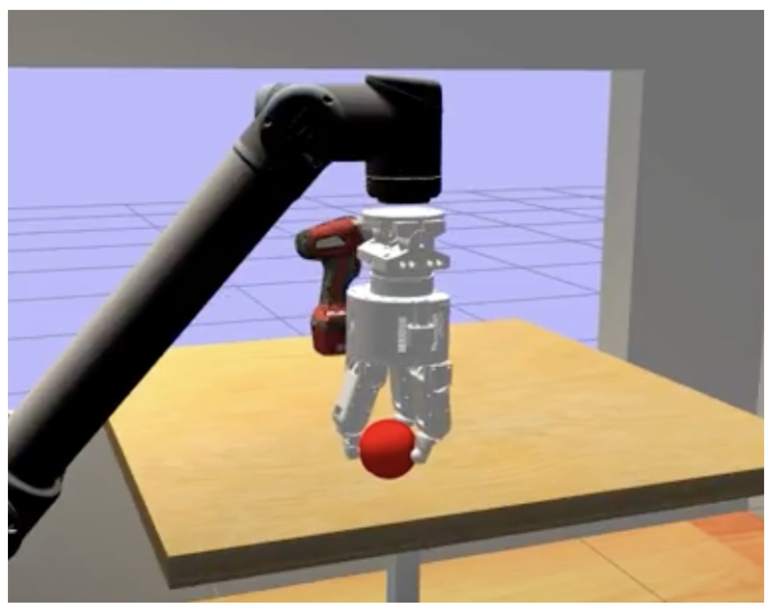
The grasp robustness
R for each experiment is computed based on the variation of the distance between the palm and the ball during the shake, as shown in
Figure 2, denoted as
where
f is a function that computes the robustness based on the distance variation
during the experiment
. By having all these features as a dataset
, then, let
be a sample from a distribution
in a domain
, where
is the instance space and
is the label space. We learn a differentiable
predictive function
together with a transparent
explainer function
defined over a functional class
. We refer to functions
,
, and
as the
predictor,
global explainer and
local explainer, respectively.
is strictly constrained to be an inherently explainable functional set, such as a set of linear functions.
Our goal is to optimize the predictor to provide global explanations that are faithful to the model’s behavior and consistent with the explanations generated by the global explainer . Then, we fine-tune the global explainer within the local neighborhood, , of a new testing instance to obtain the local explainer . We aim to achieve this by minimizing the divergence between the outputs of the predictor and global explainer in the local neighborhood while maintaining the predictor’s accuracy and generating local explanations from the local explainer model, .
3.1. Local Explainability Using Neighborhoods
Local explainability refers to understanding and interpreting a model’s predictions at an individual instance level, whereas global explanations provide an overall understanding of the model’s behavior. Thus, local explanations can offer insights into the factors influencing a specific prediction, which is particularly valuable in domains where decisions have significant consequences, such as robotics.
To achieve local explainability, we leverage the concept of neighborhoods. For each instance in the dataset, we identify a set of neighboring instances, typically using a distance metric such as k-nearest neighbors (k-NN). The intuition behind considering local neighborhoods is that similar inputs are expected to have similar outputs, and by focusing on the local neighborhood of an instance, we can capture the model’s behavior near that instance.
This neighborhood-based approach to local explainability has several advantages:
Context Awareness: By considering instances that are similar to the target instance, the explanation reflects the model’s behavior in the specific region of the feature space, accounting for local patterns and interactions that may differ from the global behavior.
Stability: Explanations based on neighborhoods tend to be more stable than those based on individual instances, as they aggregate information from multiple similar data points, reducing the impact of noise or outliers.
Generalizability: The neighborhood-based approach can be applied to various types of models and data, making it a versatile framework for local explainability.
We used the Jensen–Shannon divergence to measure the local fidelity between the predictor model and the explainer model. Specifically, we computed the JS divergence between the predictions of the predictor model and the explainer model within the local neighborhood of each instance. This allows us to quantify how well the explainer captures the predictor’s behavior in the vicinity of specific instances.
The concept of local neighborhoods also aligns well with the nature of robotic grasping, where the system operates in a high-dimensional state space with complex dynamics. By focusing on local explanations, we can provide insights that are directly relevant to specific grasping scenarios, helping robotics engineers understand the factors influencing success or failure in particular contexts.
Next, we will formalize the problem of local explainability in robot grasp failure prediction and detail our proposed approach for extending the pre hoc explainability framework to incorporate local explanations.
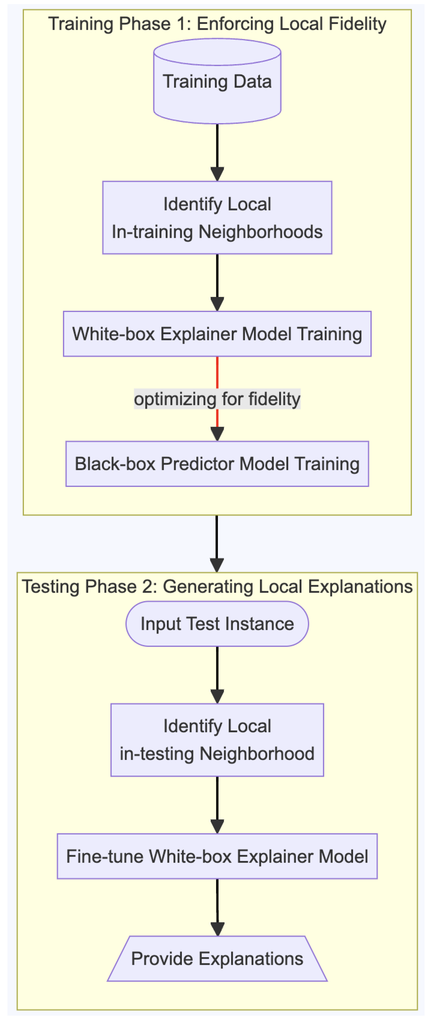
We implement a locally explainable machine learning framework, a pre hoc local explainability framework; see
Figure 3. The framework consists of 2 phases by integrating local neighborhoods to achieve local explainability. Phase 1 (training for fidelity) is the training phase that optimizes the agreement between the white-box explainer and black-box models, quantified by the fidelity with respect to the neighboring training instances. Phase 2 (generating local explanations) performs fine-tuning of the white-box explainer model within the neighboring training instances closest to a new test instance.
We use a nearest neighborhood algorithm to identify a set of neighboring instances for each local instance in the dataset, such as k-nearest neighbors (k-NN) with Euclidean distance. The intuition behind considering local neighborhoods is that similar inputs are expected to have similar outputs while capturing the model’s behavior near each instance by focusing on the local neighborhood.
We compute the predicted probability distributions for each instance and its corresponding neighbors using the predictor model and the explainer model . This step results in multiple probability distributions for each training instance, representing the predictions of the black-box and white-box explainer models within the local neighborhood. Then, we use the Jensen–Shannon divergence, computed between the predictions of the black-box predictor model and the explainer model for the local in-training neighborhoods surrounding an instance. This divergence measure quantitatively assesses the consistency between the predictor and explainer models at the local level.
3.2. Neighborhood Fidelity Objective Function
Algorithm 1 presents the method for integrating the Jensen–Shannon divergence for local explainability within neighborhoods during the training of the black-box model. The algorithm takes as input the black-box model
, the white-box model
, the training dataset
with their true labels
y, and the hyperparameter
. It also requires the nearest neighborhood function
and the number of neighborhood instances
k.
| Algorithm 1 Training phase for pre hoc: integrating local explainability with neighbors in training. |
Require: input training instances , true label y, nearest neighborhood function , number of neighborhood instances k, and parameter , the coefficient for the explainability regularization term. for each in do ▹ Get k-NN to training instance from Training set end for Initialize and for each in do Compute ▹ Predictions from predictor model Compute ▹ Predictions from explainer model Compute Compute ▹ White-box model loss ▹ Black-box model loss Update using gradient descent on : Update using gradient descent on : end for Return and procedure(, , ) ▹ Compute average JS divergence for input subset for All do end for return end procedure
|
Given a global explainer model
with parameters
, let its predictions result in a probability distribution
. Given the predictor,
with parameters
, let its predictions result in probability distribution
over binary classes
, where 1 represents a stable grasp and 0 represents an unstable grasp. We propose a neighborhood fidelity objective function, which measures the probability distances of local in-training neighborhoods
of instance
i, between
and
, which are respectively the outputs of
and
for all given input training data
. The optimization problem is formulated as follows:
where function
is a divergence distance measurement, specifically the Jensen–Shannon divergence, to measure the within-neighborhood deviation between the predictive distributions of
and
.
The Jensen–Shannon divergence between the predictions of the predictor model and the explainer model within a local neighborhood is given by
We thus define our neighborhood fidelity objective function,
, that is calculated using the Jensen–Shannon divergence (JS) as follows:
Here, represents an instance and its neighbors, f denotes the predictor’s output, and denotes the global explainer’s prediction. The difference between these two terms measures the variability in the predictions within a local neighborhood.
4. Experiments
4.1. Dataset and Preprocessing
We evaluate the performance of our local pre hoc explainability framework on the grasping dataset obtained from Shadow’s Smart Grasping System [
46] simulation with ROS [
47] and Gazebo [
48] environments using the Smart Grasping Sandbox. The dataset contains data obtained from the three 3-DOF fingers, with information about the joints’ position, velocity, and effort (torque) of each finger, amounting to about 54,000 unique data points and 29 measurements for each experiment.
The classification target is the predicted grasp robustness, which is discretized into a binary label: 1 for a stable grasp and 0 for an unstable grasp. A grasp is considered stable if the robustness value exceeds 100. The dataset was normalized using standard scaling to ensure that each feature contributes equally to the prediction.
4.2. Experimental Protocol
The dataset was randomly divided into training, validation, and test sets with an 80:10:10 ratio. All experiments were repeated five times, and the results were averaged across the five runs and reported along with the standard deviation. All models were trained with regularization until validation accuracy stabilized for at least ten epochs. For local explainability neighborhood generation, we experimented with different neighborhood sizes. We set the number of neighbors during the training phase (Phase 1: training for fidelity) and explored different values of during the testing phase (Phase 2: generating local explanations) to analyze the impact of neighborhood size on explanation quality and computational cost.
The models were implemented using the PyTorch v2.6 framework [
49] and executed on an NVIDIA Tesla V100 GPU with 16 GB RAM and an Intel(R) Xeon(R) CPU with 2.20 GHz and 13 GB RAM. We also conducted experiments that compared CPU and GPU performance for both training and explanation generation.
4.3. Models and Baselines
We compared our local pre hoc explainability framework with the following baselines.
Black-Box (BB) Predictor: A non-regularized factorization machine model that serves as the baseline for prediction accuracy.
White-Box (WB) Explainer: A sparse logistic regression model that serves as the explainer.
LIME [
21]: A popular post hoc explanation method that generates local explanations by training interpretable models on perturbed samples.
For our pre hoc framework, we experimented with different values of the explainability regularization parameter to analyze the trade-off between prediction accuracy and explanation fidelity.
4.4. Evaluation Metrics
We evaluate our approach using the following metrics for both prediction accuracy and explanation quality.
4.4.1. Prediction Accuracy
To assess the classification accuracy, we use the Area under the ROC Curve (AUC), . This metric measures the model’s ability to correctly classify grasp stability across different threshold values.
4.4.2. Global Explanation Fidelity
To evaluate how well the explainer model captures the global behavior of the predictor model, we use the fidelity metric: . This measures the agreement between the predictor model’s predictions and the explainer model’s predictions across the entire test set.
4.4.3. Local Explanation Metrics
To evaluate the quality of local explanations, we use the following key metrics.
Definition 1 (Point Fidelity (PF)).
Measures the agreement between the explanations and predictions for an individual instance:A higher point fidelity is better.
Definition 2 (Neighborhood Fidelity (NF)).
Extends the concept of point fidelity to consider agreement within the local neighborhoods around each instance:A higher neighborhood fidelity is better.
Definition 3 (Stability).
Measures the consistency of explanations across different runs or small perturbations of the input:where d is a distance function (Euclidean) between the explanations and are explanations generated from slightly perturbed versions of the same instance. A lower stability is better.
5. Results and Discussion
In this section, we present and analyze the results of our experiments on the grasping dataset to evaluate the effectiveness of our local pre hoc explainability framework. We organize our findings according to the research questions outlined in Section Research Questions and Contributions.
5.1. RQ 1—Explanatory Power: How Well Does the Explainer Model Mimic the Predictor Model in Phase 1?
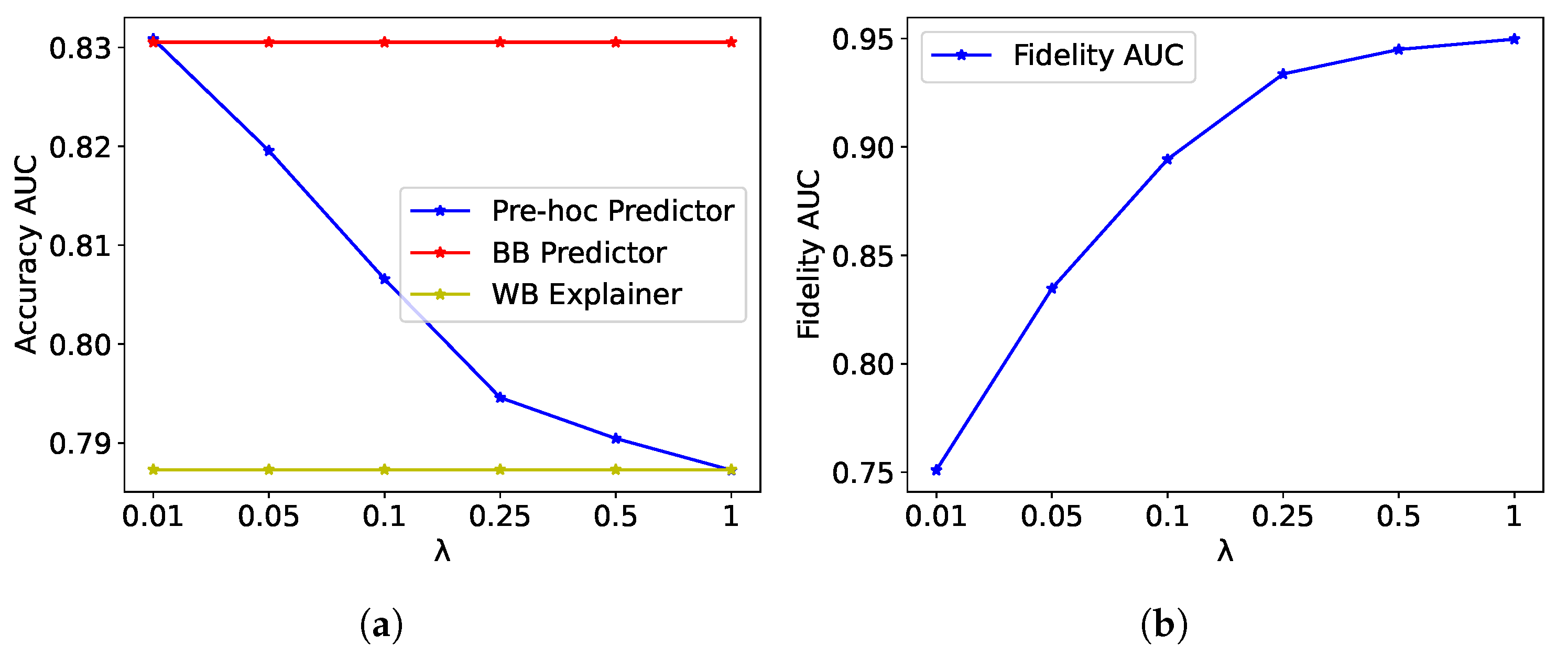
To assess the global explanatory power of the pre hoc framework, we examined how well the explanations generated by the framework capture the nuances of the black-box model’s decision-making process by analyzing the fidelity AUC scores for different values of the explainability regularization parameter .
Figure 4b presents the fidelity AUC scores for the pre hoc framework on the grasping dataset for different values of
. As
increases, the fidelity AUC shows a notable improvement, increasing from around 0.80 at
to approximately 0.95 at
. This indicates that higher values of
strengthen the regularization effect, encouraging the Pre Hoc Predictor to align more closely with the WB Explainer. Since the WB Explainer is used to guide the learning of the Pre Hoc Predictor, the high fidelity scores suggest that the explanations generated by the pre hoc framework effectively capture the nuances of the black-box model’s decision-making process.
The high fidelity scores achieved by the proposed framework demonstrate the effectiveness of using the WB Explainer to guide the learning of the black-box predictor and generate explanations that align closely with the model’s decisions. The results indicate that our pre hoc framework can produce explanations that faithfully represent the model’s decision-making process, which is essential for building trust in the predictions of grasp failure in robotic systems.
5.2. RQ 2—Trade-Off Between Accuracy and Explanation Fidelity: How Does Explainability Regularization Affect the Accuracy and Fidelity Score in Phase 1?
To analyze the effect of the explainability regularization parameter on the accuracy and fidelity scores, we examined how varying affects both prediction performance and explanation quality.
Figure 4a displays the accuracy based on AUC scores for the Pre Hoc Predictor, BB Predictor, and WB Explainer models, evaluated on the grasping test set for different values of
. As
increases from 0.01 to 1, the AUC of the Pre Hoc Predictor remains relatively stable, with a slight decrease from around 0.83 to 0.81. The AUC of the Pre Hoc Predictor is consistently higher than that of the WB Explainer, demonstrating that the pre hoc framework maintains a good balance between accuracy and explainability. The BB Predictor, which is the unregularized black-box model, has a slightly higher accuracy than the Pre Hoc Predictor, but the difference is minimal.
These results demonstrate the effectiveness of the explainability regularization parameter in controlling the trade-off between accuracy and explainability in the pre hoc framework. Lower values of prioritize prediction accuracy, whereas higher values emphasize explainability. The choice of depends on the specific requirements of the application and the desired balance between accuracy and interpretability. With high values of , the accuracy of the Pre Hoc Predictor remains competitive with that of the BB Predictor on the grasping dataset, indicating that the pre hoc framework effectively incorporates explainability without significantly compromising predictive performance.
Table 2 provides a comparison of the different models in terms of prediction accuracy (AUC) and explanation fidelity. The results show that as
increases from 0.01 to 0.1, the fidelity improves significantly from 0.786 to 0.956, at the cost of a slight decrease in accuracy from 0.833 to 0.812. This represents a trade-off between prediction performance and explanation quality, with a modest 2.5% decrease in accuracy leading to a substantial 21.6% increase in fidelity. The pre hoc framework with
provides a good balance, with an accuracy of 0.824 and a fidelity of 0.872.
5.3. RQ 3—Locality: How Well Do the Explanations Capture the Local Behavior of the Model Compared to LIME in Phase 2?
To assess the local explainability of our proposed framework, we compared its performance with the LIME post hoc explainability method in terms of point fidelity, neighborhood fidelity, and stability.
Table 3 shows the comparison results between our pre hoc framework and LIME. Our pre hoc framework significantly outperforms LIME in terms of point fidelity (0.917 vs. 0.700), neighborhood fidelity (0.960 vs. 0.741), and stability (0.022 vs. 0.215). These results indicate that our pre hoc framework generates explanations that are more faithful to the model’s predictions and more consistent across different runs compared to LIME.
The high point fidelity and neighborhood fidelity scores of our pre hoc framework indicate that the generated explanations are consistent with the model’s predictions for individual instances and within local neighborhoods. The low stability score suggests that our framework produces more consistent explanations across different runs compared to LIME. This is particularly important in robotics applications, where the reliability and consistency of explanations are crucial for building trust in the system.
The superior performance of our pre hoc framework can be attributed to the fact that it incorporates explainability during the training phase, ensuring that the model’s predictions are inherently aligned with its explanations. In contrast, LIME, being a post hoc method, attempts to explain the model’s decisions after the fact, which can lead to less faithful and less consistent explanations.
5.4. RQ 4—Neighborhood Size: How Does Neighborhood Size Affect Neighborhood Fidelity, Stability, and Computational Cost in Phase 2?
To understand the impact of neighborhood size on explanation quality and computational cost, we conducted experiments with different values of k in Testing Phase 2.
Table 4 presents the results of our experiments with different neighborhood sizes during Testing Phase 2. As the neighborhood size increases from 3 to 100, we observe the following trends.
Neighborhood fidelity increases from 0.883 for to 0.967 for . This indicates that larger neighborhoods better capture the local patterns and provide more accurate explanations.
Stability decreases significantly from 0.215 for to 0.002 for . A lower stability value indicates more consistent explanations across different instances within the neighborhood. This suggests that larger neighborhoods provide more stable explanations.
Computation time increases slightly from 0.012 s for to 0.014 s for . The difference is minimal, indicating that the computational cost is not significantly impacted by the choice of neighborhood size, at least within the range of values considered.
These results provide valuable insights for selecting the appropriate neighborhood size for generating local explanations in robotic grasp failure prediction. If the primary concern is explanation quality and stability, larger neighborhood sizes (e.g., ) are preferable. If computational efficiency is a priority, smaller neighborhood sizes (e.g., or ) can be used without significantly compromising explanation quality. In our experiments, provides a good balance between explanation quality and computational cost.
5.5. Local Explanation Example for Grasping Dataset
To provide a concrete example of the local explanations generated by our pre hoc framework, we present a case study of an individual test instance from the grasping dataset.
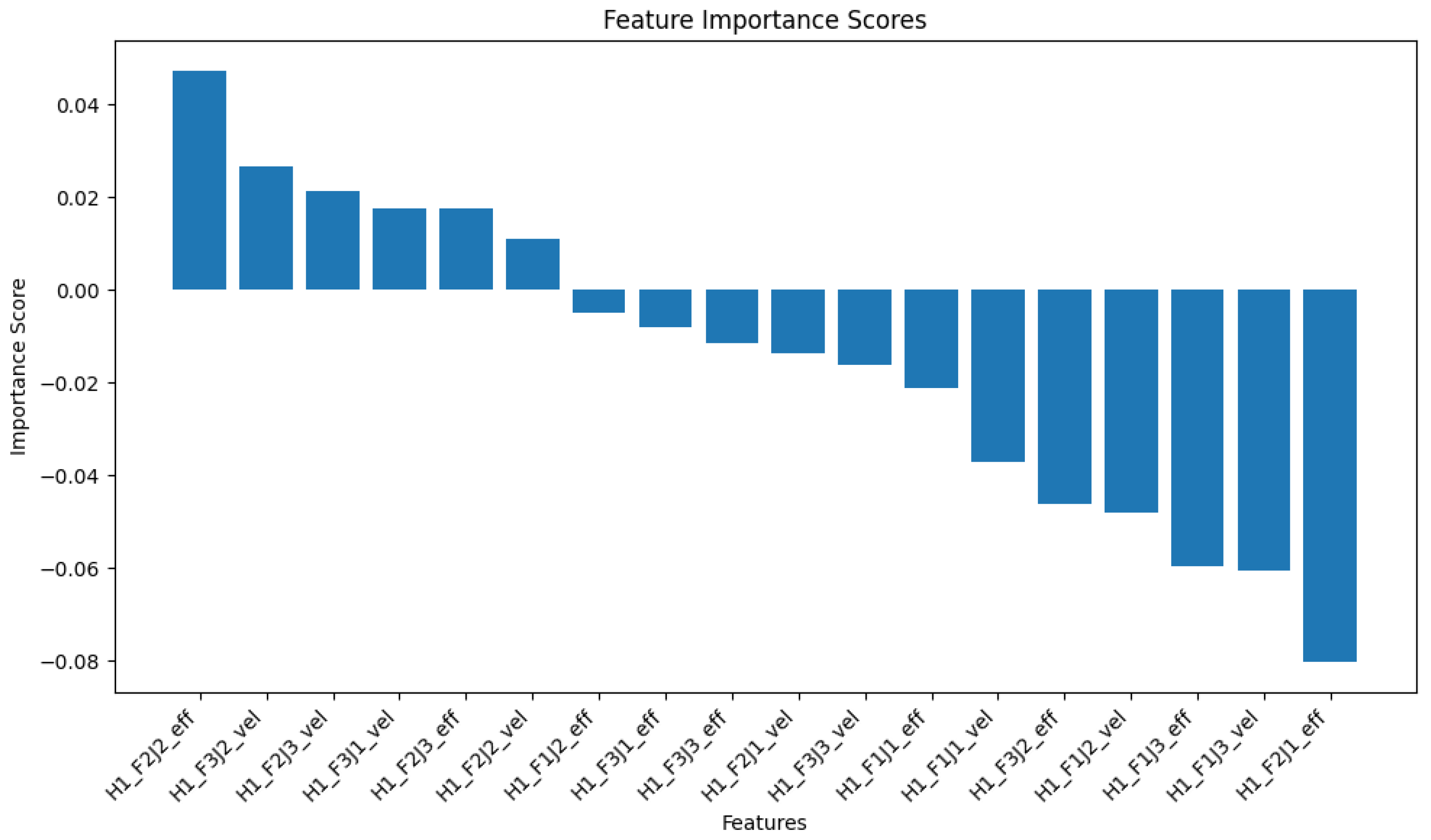
Figure 5 illustrates the local feature importance scores for a specific test instance from the grasping dataset. The explanation highlights the most influential features for this particular prediction, providing insights into the factors contributing to the model’s decision.
For this specific instance, the explanation reveals that both effort and velocity features have significant impacts on the prediction, with varying directions of influence. This level of granularity in the explanation provides valuable insights for robotics engineers to understand the specific factors affecting grasp stability for individual scenarios, which can guide improvements in grasping strategies.
5.6. Global Explainability Insights
While our focus in this paper is on local explainability, it is worth noting the global patterns identified by our pre hoc framework in the grasping dataset.
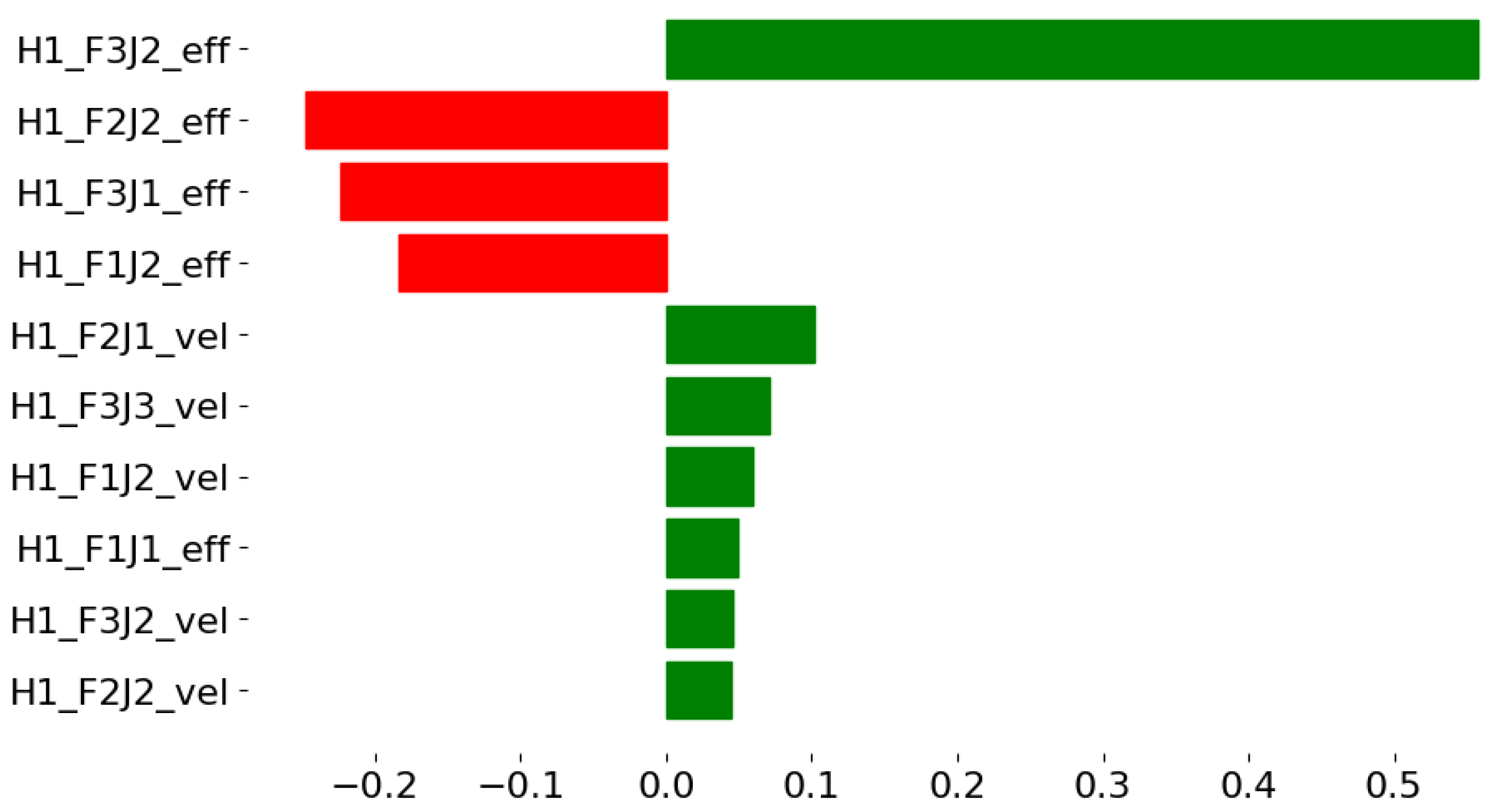
Figure 6 shows the top 10 global feature importance scores for the grasping dataset. The most influential feature is H1F3J2eff (effort exerted in Joint 2 of Finger 3), which increases the likelihood of grasp failure. In contrast, the efforts exerted on Joint 2 of Fingers 1 and 2 and Joint 1 of Finger 3 reduce the probability of grasp failure. These global patterns provide general information on the factors that affect grasp stability in all instances.
Comparing the local explanation (
Figure 5) with the global explanation (
Figure 6), we observe similarities and differences. Although the global explanation emphasizes the importance of effort features over velocity features, the local explanation shows a more mixed impact of both types of feature. This confirms the value of local explanations in capturing instance-specific patterns that can deviate from global trends.
Our pre hoc framework provides both global and local explainability, offering a comprehensive understanding of the model’s behavior at different levels of granularity. This multilevel explainability is particularly valuable in robotics applications, where both general patterns and instance-specific insights are essential for designing robust and reliable systems.
5.7. Limitations and Future Directions
While our experimental evaluation demonstrates the effectiveness of the proposed local pre hoc explainability framework, it is important to acknowledge the limitations of the dataset and discuss the generalization potential of our results to broader robotic grasping scenarios. The dataset is limited to grasping tasks performed in a static Gazebo simulation environment with consistent lighting and no external disturbances. Real-world grasping scenarios present additional challenges, including sensor noise, varying lighting conditions, occlusions, and dynamic environments. Although simulation provides safe, low-cost, and controlled conditions for systematic evaluation, there is an inherent gap between simulated and real-world robotic systems. Factors such as mechanical compliance, sensor accuracy, actuator dynamics, and physical wear are simplified or idealized in simulation. The transition from simulation to real robotic platforms may introduce additional failure modes and sources of uncertainty that are not captured in the current dataset. Sparse neighborhoods could cause failures. When local neighborhoods contain fewer than 3–5 training instances, the quality of the explanation may be degraded, where unusual sensor combinations (e.g., extremely high joint efforts combined with very low velocities) may result in sparse local neighborhoods. Our method assumes that local neighborhoods contain instances with similar underlying causal relationships. This assumption may be violated in complex robotic environments where subtle changes in object properties or environmental conditions create non-obvious feature interactions.
Our implementation uses the scikit-learn k-nearest neighbors model with Euclidean distance as the default metric for neighborhood construction. Although the Euclidean distance is computationally efficient and appropriate for continuous sensor data, we acknowledge that systematic evaluation of alternative distance metrics (such as the Mahalanobis, Manhattan or Cosine distance) and their impact on neighborhood quality and explanation fidelity would provide valuable insights into optimal distance metric selection for different types of robotic sensor data and represent an important direction for future research.
Furthermore, our current analysis focuses primarily on an ablation study and a comparison with LIME as the main baseline for local explainability. A more comprehensive evaluation comparing computational performance with additional explainability methods such as SHAP, Integrated Gradients, and other local explanation techniques would provide a broader perspective on our framework’s efficiency advantages and represent an important direction for future work.
Although we acknowledge these limitations, the controlled evaluation demonstrates the fundamental viability of our local explainability approach for robotic grasping applications. Significant improvements in explanation fidelity, stability, and computational efficiency suggest that the framework provides a solid foundation for deployment in practical scenarios, with appropriate domain-specific adaptations and additional validation as systems transition from controlled to operational environments.
6. Conclusions
In this paper, we extended our recently proposed pre hoc explainability framework [
23] to incorporate local explainability for robot grasp failure prediction. By leveraging neighborhood information and the Jensen–Shannon divergence, our approach generates instance-specific explanations that capture the model’s decision-making process for individual grasp scenarios. The two-phase methodology first trains the predictor model with local explainability constraints, then fine-tunes the pre-trained explainer for each test instance within its local neighborhood, resulting in explanations with superior point fidelity, neighborhood fidelity, and stability compared to traditional post hoc methods like LIME.
Future work could extend this framework to multiclass classification or regression problems for predicting continuous measures of grasp quality, explore alternative explanation formats beyond feature importance scores, and incorporate temporal data to explain dynamic grasping processes. Additional validation on different robotic platforms and integration of domain knowledge from robotics experts would further enhance the framework’s applicability. Despite these opportunities for improvement, our local pre hoc explainability framework represents a significant advancement in transparent and interpretable robot grasp failure prediction, enhancing trust in autonomous robotic systems while providing valuable insights for improving grasping strategies.


