Article

A Neural Network Compiler for Efficient Data Storage Optimization in ReRAM-Based DNN Accelerators

1
Department of Electronic Engineering, Chung Yuan Christian University, Taoyuan 320314, Taiwan
2
Department of Information and Computer Engineering, Chung Yuan Christian University, Taoyuan 320314, Taiwan
*
Author to whom correspondence should be addressed.
Electronics 2025, 14(12), 2352; https://doi.org/10.3390/electronics14122352
Submission received: 1 May 2025 / Revised: 3 June 2025 / Accepted: 6 June 2025 / Published: 8 June 2025
(This article belongs to the Special Issue Research on Key Technologies for Hardware Acceleration)

Abstract

:
ReRAM-based DNN accelerators have emerged as a promising solution to mitigate the von Neumann bottleneck. While prior research has introduced tools for simulating the hardware behavior of ReRAM’s non-linear characteristics, there remains a notable gap in high-level design automation tools capable of efficiently deploying DNN models onto ReRAM-based accelerators with simultaneous optimization of execution time and memory usage. In this paper, we propose a neural network compiler built on the open-source TVM framework to address this challenge. The compiler incorporates both layer fusion and model partitioning techniques to enhance data storage efficiency. The core contribution of our work is an algorithm that determines the optimal mapping strategy by jointly considering layer fusion and model partitioning under hardware resource constraints. Experimental evaluations demonstrate that the proposed compiler adapts effectively to varying hardware resource limitations, enabling efficient storage optimization and supporting early-stage design space exploration.

1. Introduction

In recent years, artificial intelligence (AI) has been widely applied in fields such as healthcare, computer vision, and natural language processing. To address various data characteristics, numerous deep neural network (DNN) models have been developed to process and analyze large volumes of data, for instance, convolutional neural networks (CNNs), which are primarily employed in image processing and computer vision. To improve performance, many CNN architectures have been proposed [1,2,3,4,5,6,7]. As CNN scales up rapidly, their architectures have become increasingly complex. Since CNN comprises multiple convolutional layers, each requiring extensive computations, enhancing computational efficiency has become paramount.
To enable developers to efficiently construct, train, and deploy DNN models while optimizing computational performance and resource utilization, several widely adopted deep learning frameworks have been introduced, including PyTorch [8], TensorFlow [9], MXNet [10], and Caffe [11]. However, deploying models created with different frameworks onto target hardware platforms still requires substantial effort. In particular, to satisfy real-time constraints such as low latency and high throughput, a range of DNN accelerators, including GPUs, Google’s TPU [12], Nvidia Jetson, FPGAs, and various ASICs, are commonly employed. Although these DNN accelerators can greatly enhance the performance of neural network computations, effectively mapping models onto diverse hardware platforms also necessitates the use of efficient and adaptable compilers.
Foundational studies and overviews of classical optimization methods can be found in [13,14]. Deep learning frameworks typically incorporate a variety of general-purpose libraries that assist developers in building and optimizing DNN models. For example, convolution operations can be reformulated as matrix vector multiplications (MVMs) using basic linear algebra subprograms (BLAS), enabling efficient execution through the general matrix multiplication (GEMM) functions provided by these libraries. In addition to general-purpose solutions, many neural network accelerator vendors offer specialized libraries tailored for DNN workloads: TensorRT, for example, supports graph-level optimizations and low-precision quantization, while other libraries [15,16] target specific accelerator architectures. However, the rapid pace of innovation in deep learning has made it challenging for library development to keep up with the evolving demands of DNN accelerator users.
To alleviate the burden of manually optimizing neural network models for each DNN accelerator, several deep learning compilers, such as Glow [17], nGraph [18], and TVM [19], have been introduced. These compilers accept models defined in deep learning frameworks and apply optimizations tailored to both the model characteristics and the target hardware architecture, ultimately generating code that executes efficiently on a variety of DNN accelerators. Moreover, many of these compilers are built on top of well-established tool chains from general-purpose compilers, such as LLVM [20], which further enhances their portability across different accelerator platforms.
While deep learning compilers streamline the deployment of DNN models onto hardware accelerators, their optimizations are largely software-centric, leaving significant opportunities to enhance hardware utilization. Given that storage space in each processing element (PE) is a critical hardware constraint, this paper focuses on optimizing on-chip data storage usage and addresses two key issues:
  • Layer Fusion: If a PE has sufficient storage space to hold the data required for two or more layers, we use layer fusion to make full use of its storage capacity.
  • Model Partitioning: If a PE’s storage space is insufficient to accommodate the data required by a single layer, we partition the computations of that layer and distribute them across multiple PEs for concurrent execution.
On the other hand, there have also been several advances in DNN accelerator design in recent years. In general, most DNN accelerators have focused on architectural improvements in three main directions: systolic arrays [21,22,23], network-on-chip (NoC) designs [24,25,26], and reduced tree structures [27]. Furthermore, some research has explored specialized architectural designs; for example, Ref. [28] proposes methods that simplify computation and reduce latency, while [29,30] utilize compression techniques to save memory. Other studies have introduced techniques such as optimizing activation functions [31] to reduce processing latency in DNN accelerators. However, these hardware designs still follow the von Neumann architecture, which suffers from performance bottlenecks as a result of heavy data transfer. Although various approaches have been proposed to mitigate these bottlenecks, such as analyzing dataflows to minimize data transfers [32,33,34] or employing approximate computing to reduce power consumption and data traffic [35,36,37,38], they remain constrained by the fundamental limitations of the von Neumann architecture and do not fully resolve the issue of data transfer.
In-memory computing has gained wide recognition as a promising strategy for addressing the von Neumann bottleneck. In particular, previous work [39,
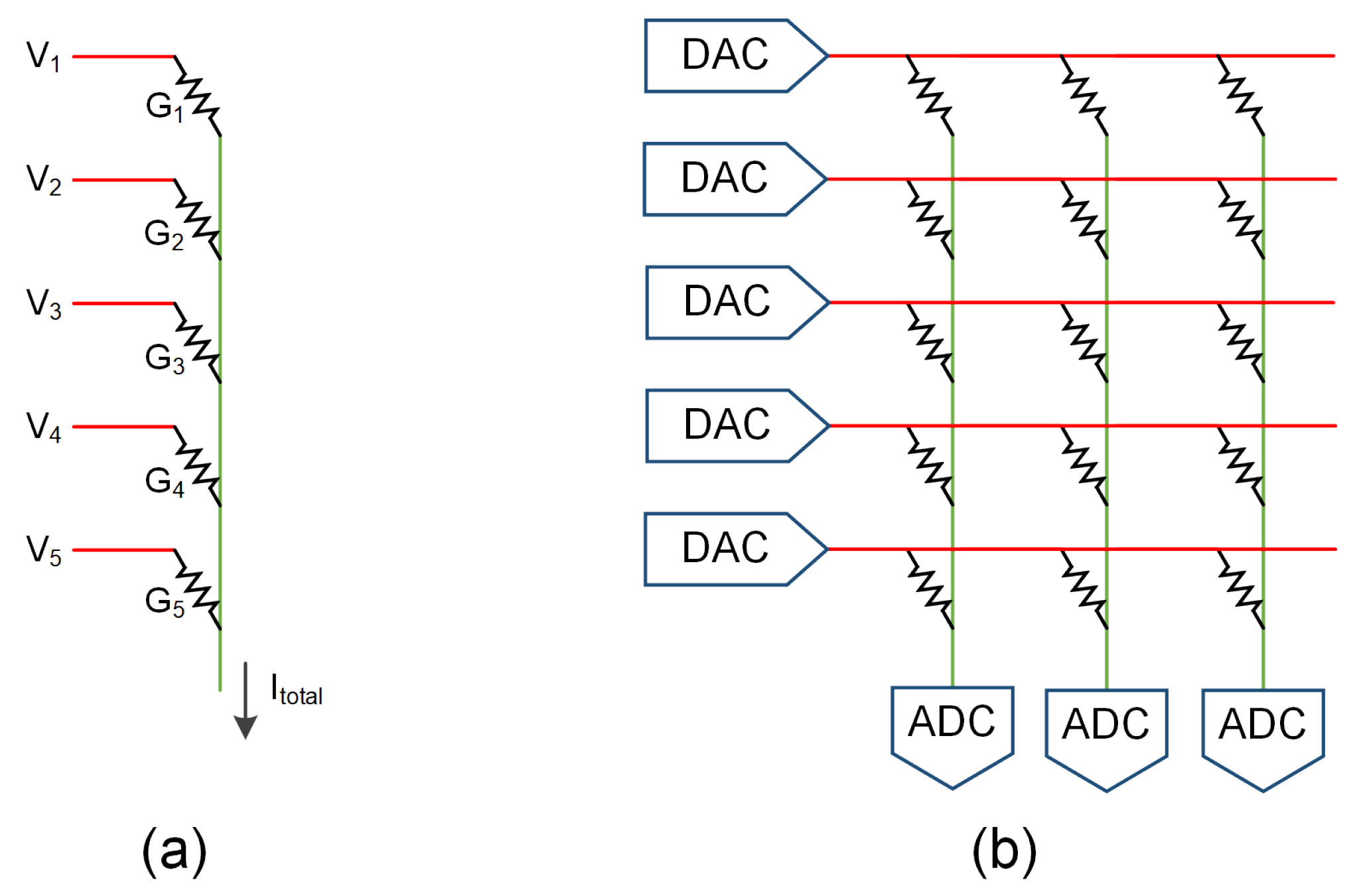
40] introduced pioneering memristor-based DNN accelerators that significantly reduce both data movement and power consumption during neural network computations. Unlike conventional von Neumann architectures that separate computation and data storage, these accelerators execute MVMs directly in memory, thereby enhancing energy efficiency. In this architecture, input activations are first converted into analog signals, while weights are stored within memory cells; the dot product is performed in situ, substantially minimizing data transfer. As shown in [41], metal–oxide resistive RAM (ReRAM) can be assembled into crossbar arrays to efficiently handle MVM operations in both convolutional and fully connected layers. Furthermore, due to their multilevel storage capabilities, compact area footprint, and low read/write latencies, ReRAM-based memory arrays have emerged as one of the most effective hardware solutions for DNN acceleration [42,43,44,45,46]. Several tools have been introduced to facilitate high-level design for ReRAM-based DNN accelerators. For example, Ref. [47] examines the weight mapping and data flow within these accelerators, while [48] simulates the hardware behavior of the nonlinear characteristics of ReRAM in the high-level design stage. However, the development of deep learning compilers specifically tailored for ReRAM-based DNN accelerators remains largely unexplored.
In this paper, we present a deep learning compiler specifically tailored for ReRAM-based DNN accelerators, based on the open-source TVM framework [19]. Our primary objective is to optimize the usage of data storage. To achieve this, our core contribution is an approach that determines the optimal mapping strategy by jointly applying layer fusion and model partitioning, while accounting for the storage constraints of each PE. By integrating these two techniques, we reduce the data transfer overhead between off-chip and on-chip memory, thereby enhancing the execution efficiency of neural network models on ReRAM-based DNN accelerators. The experimental results show that our compiler effectively optimizes data storage under a variety of hardware configurations, allowing designers to accurately evaluate DNN models at an early stage in the design process.
The contributions of this paper are elaborated as follows:
  • We present the first approach to integrate layer fusion and model partitioning into TVM’s graph-level compilation stage.
  • Building on this integration, we propose an algorithm that tailors data storage optimization to multiple objectives.
The remainder of this paper is organized as follows. Section 2 introduces the background materials, and Section 3 discusses our motivation. Section 4 presents the proposed algorithm, which combines layer fusion and model partitioning. Section 5 provides the experimental results. Finally, Section 6 offers concluding remarks.

2. Preliminaries

In this section, we review the relevant background. Section 2.1 provides a brief overview of CNNs, Section 2.2 introduces the ReRAM-based DNN accelerator [48], and Section 2.3 summarizes the TVM framework [19].

2.1. Convolutional Neural Networks (CNNs)

Within CNNs, convolutional layers play a crucial role in extracting information from input feature maps. Figure 1 illustrates a conceptual diagram of a two-dimensional CNN, where the network input activation is a four-dimensional tensor. Specifically, in Figure 1, the input feature maps are represented by H, W, and C, with H denoting the height, W the width, and C the number of channels, while N indicates the number of feature maps input at one time. In Figure 1, the convolution operation is performed using a convolution kernel characterized by R, S, and M, where R, S, and M represent the height, width, and number of kernels, respectively.
During the convolution process, each convolution kernel slides across all feature maps to generate multiple dot products. After processing, these dot products produce an output feature map with dimensions E × F and M dimensions, which are then passed as input activations to the next layer. Note that the channel dimension of the input feature map is identical to that of each convolution kernel, and the number of convolution kernels determines the channel dimension of the output feature map.
However, convolution involves a tremendous amount of data computation and high data throughput. To enhance operational efficiency, it is necessary to design an efficient DNN accelerator capable of handling these large-scale MVMs to perform 2D convolution. As described in [24], the dataflows of conventional digital DNN accelerators can be categorized into several schemes, including input reuse, weight stationary, partial sum stationary, and the row-stationary approach. In general, input activations stored in memory are arranged in the order N, C, H, and W, while the weight values are stored in the order M, R, and S. This storage scheme may be suitable for general-purpose neural network accelerators or GPUs; however, for in-memory computations, data flow constraints may arise, necessitating the design of data flow schemes in accordance with the hardware limitations.
Figure 2 illustrates an ideal mapping of the convolution operation from Figure 1 into memory operations. Here, the input activations have dimensions H × W × C, the convolution kernel has dimensions R × S × C × M, and the output has dimensions E × F × M. Due to the limitations of CIM architectures, each kernel is typically stored as an R × S × C block in a single row, resulting in M rows corresponding to different kernels. Generally, a PE in a DNN accelerator comprises multiple memory arrays. In [47], to enhance operational efficiency, the convolution operation of the entire input feature map is distributed across different memory sub-arrays within a PE, with each sub-array using the same set of weight values. Each sub-array then produces one pixel of the output feature map, and by combining the outputs from all sub-arrays, the complete output feature map is obtained, as shown in Figure 3.

2.2. ReRAM-Based DNN Accelerators

Due to its low read/write latency, ReRAM is particularly well suited for in-memory-computing applications. Moreover, ReRAM can store multiple bits of data per cell at a relatively low area cost. Figure 4 illustrates the basic concept of performing CIM operations using a ReRAM array. In Figure 4a, a column of the ReRAM array is shown where the weights for the convolution operation are pre-stored in ReRAM cells and represented as conductance values. Meanwhile, the input to the convolution is converted into a voltage using a digital-to-analog converter (DAC), as shown in Figure 4b. According to Ohm’s law I = V R = V × G , the computation within a ReRAM cell can be expressed as
I = V × G ,
where the current I is the product of the input voltage V and the weight’s conductance G. For each column in the ReRAM array, the total current can be represented as
I t o t a l = n ( V n × G n ) ,
with I t o t a l denoting the accumulated current of that column, that is, the cumulative result of all ReRAM cells after the in-memory operation. The accumulated current I t o t a l is then converted into a digital signal via an analog-to-digital converter (ADC), as shown in Figure 4b.
Each column of the ReRAM array can be viewed as a multiply–accumulate (MAC) unit. In other words, the properties of the ReRAM array can directly emulate the behavior of a MAC. By judiciously arranging the data flow of input activation and weight values, ReRAM arrays can be used effectively as DNN accelerators [48].

2.3. The Flow of TVM

To improve the performance and efficiency of the model on different hardware platforms, an open source deep learning compiler framework called TVM was proposed in [19]. TVM is an end-to-end optimized compilation framework that transforms high-level DNN models into low-level optimized code executable on hardware platforms such as CPUs, GPUs, and DNN accelerators. Its process can be divided into four main stages, as shown in Figure 5.
  • Frontend Stage: A parser converts operations from deep learning frameworks into a relay intermediate representation (IR) module, TVM’s representation of the computation graph, thereby supporting various deep learning framework formats.
  • Graph Level: The relay IR module generated in the first stage undergoes graph-level optimizations, such as operator fusion, constant folding, and data layout transformations.
  • Tensor Level: At this stage, the relay IR module is transformed into a tensor IR module, where tensor-level optimizations are applied, including loop transformations and tensorization.
  • Code Generation and Target: The optimized code is then generated and can be deployed to hardware platforms such as CPUs, GPUs, FPGAs, or ASIC-based DNN accelerators.
Based on the TVM workflow, when DNN is deployed onto hardware, the DNN is first converted by the parser, then optimized at both the graph and tensor levels, and finally, compiled into code deployable on the target hardware. In this paper, we have integrated our proposed optimization algorithm into the graph-level compilation stage of TVM while taking into account hardware resource constraints.

3. Motivation

Generally, DNN accelerators enhance computational efficiency through improved hardware components. When a PE is defined as the acceleration unit, the TVM compiler [19] treats it as the target hardware during compilation. In the context of a CNN, each layer is regarded as a separate operation, and the TVM compiler typically maps each layer to a single PE.
Since the TVM’s approach optimizes from a software perspective, two issues may arise:
  • Insufficient On-Chip Storage in a PE: For example, as illustrated in Figure 6, when the storage capacity of a PE cannot accommodate an entire stage (i.e., a complete layer), TVM partitions the layer into multiple subunits, each processed by the PE in separate cycles. However, this approach may overlook hardware data flow considerations, potentially leading to excessive data movement and increased computational overhead. Furthermore, if a particular stage (i.e., a specific layer) cannot be executed efficiently, it can become a performance bottleneck, limiting the overall efficiency of the model.
  • Excessive On-Chip Storage in a PE: When the storage capacity of a PE exceeds the requirements of a single stage, TVM does not utilize the remaining capacity by deploying subsequent stages onto the same PE. Instead, since the compiler allocates only the data required for one layer per PE, the output of each layer must be written to external memory. When the next stage is ready for execution, these data must be reloaded into the on-chip memory. This approach under-utilizes the available storage capacity and results in reduced processing efficiency.
To address these issues, we are motivated to integrate model partitioning and layer fusion techniques into the graph-level compilation stage of TVM. The following subsections introduce the concepts behind these two approaches.

3.1. Model Partitioning

In Figure 6, a weight kernel with dimensions {3, 1, 3} and an input activation with dimensions {3, 1, 5} are subjected to a complete convolution operation at the graph level. Suppose that the on-chip storage available in a PE only supports convolution with input activations and weight kernels of dimensions {3, 1, 3}. In this case, TVM compiles the operation into three tiling steps, which are then sequentially mapped onto a single PE for execution. However, this method suffers from low operational efficiency, as it requires three separate execution cycles.
In contrast, model partitioning divides the model into multiple subgraphs at the graph level. As illustrated in Figure 7, after partitioning, the original operation is split into three parallel operations. TVM treats each subgraph as a distinct operation, and upon compilation, these operations are deployed onto different PEs within the DNN accelerator. By employing model partitioning, multiple PEs can be leveraged for parallel processing, thereby achieving higher operational efficiency while also addressing the issue of insufficient on-chip storage.

3.2. Layer Fusion

When a PE’s storage capacity exceeds the requirements of a single stage but is restricted to accelerating only one stage at a time, the DNN accelerator is not utilized efficiently. In a DNN, the output of one layer serves as the input to the next. Therefore, if the PE has sufficient storage, multiple stages should be fused and accelerated concurrently on the same PE. This layer fusion approach can significantly reduce data transfers and energy consumption.
Figure 8 illustrates the benefits of layer fusion. In Figure 8, each block in the feature map is assumed to have a size of 0.1 MB. In Figure 8a, no layer fusion is applied. Here, TVM schedules the operations of each layer on the same PE and writes the output to external memory (DRAM) upon completion. Consequently, the output of each layer must be transferred to DRAM before being reloaded for the subsequent layer. As displayed in Figure 8a, the data transfer amounts to 5.1 MB in the first stage and 2.1 MB in the second stage, resulting in a total of 7.3 MB.
In contrast, Figure 8b shows that if two consecutive layers (e.g., layer1 and layer2) are merged into a single stage, TVM arranges for the data of both layers to reside simultaneously in the on-chip memory of the PE. After performing the convolution operations for both layers, only the final result is written to the DRAM. By avoiding the transfer of intermediate output, this fused-layer approach significantly reduces both transfer time and energy consumption, thereby improving the efficiency of the DNN accelerator. As displayed in Figure 8b, the total data transfer is only 4.5 MB.
It is worth noting that both AutoTVM [49] and Ansor [50] adopt a concept similar to model partitioning, in which a tensor program expression is decomposed into multiple tasks for parallel execution. However, they [49,50] do not consider or explore the application of layer fusion.

4. The Proposed Approach

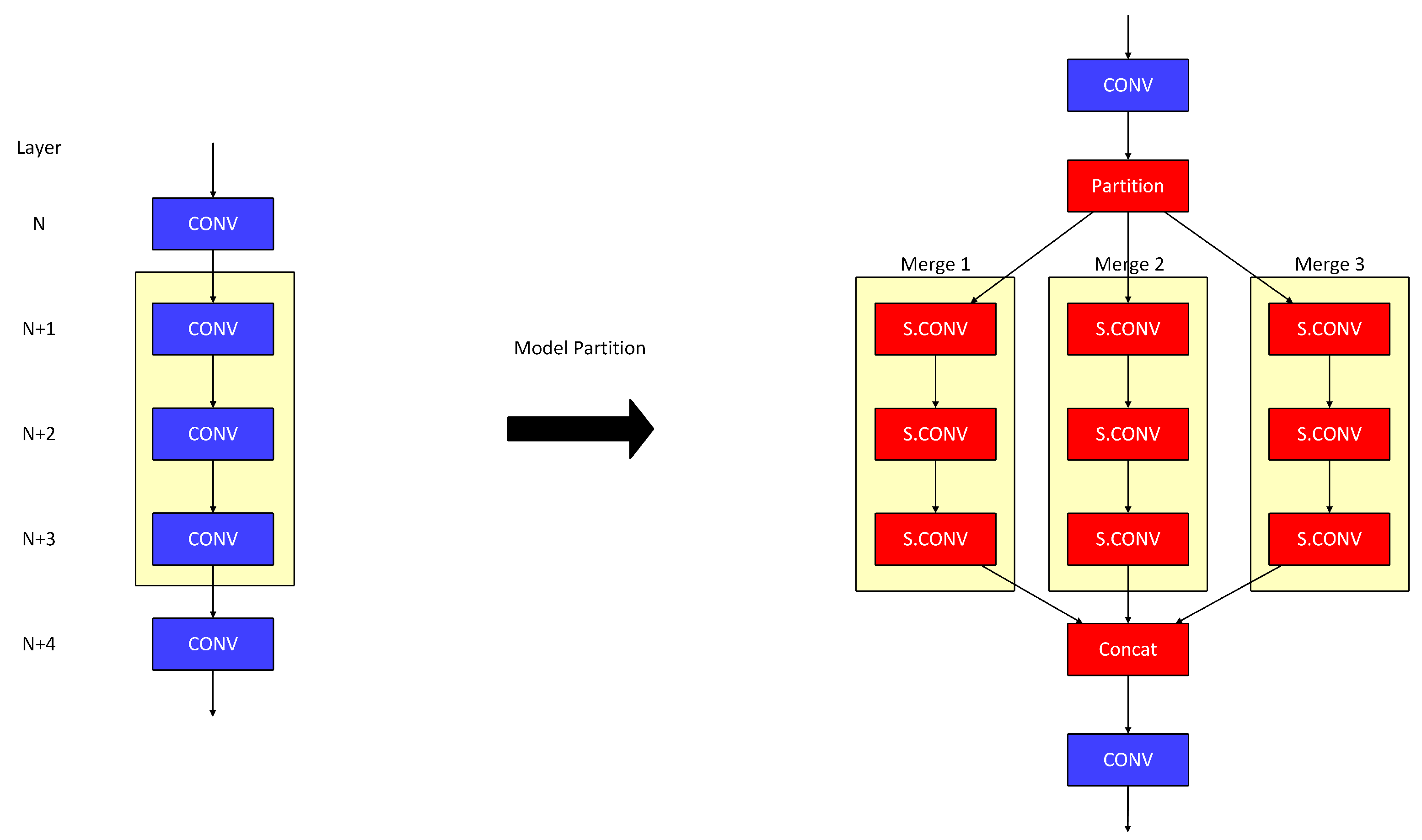
In our approach, we combine the advantages of layer fusion and model partitioning. When on-chip storage exceeds the requirements for a single stage, layer fusion merges multiple layers to reduce data transfers. In contrast, when on-chip storage is insufficient for a fused stage, the layers are partitioned into subgroups to lessen the storage demand. As illustrated in Figure 9, the left side shows the original model with five convolutional layers, while the right side demonstrates the model after the combined application of layer fusion and model partitioning.
In Figure 9, we fuse three layers of the model to reduce communication costs between off-chip memory and on-chip storage. However, this fused model requires a larger on-chip storage capacity. To address this issue, we partition the fused layers into three subgroups, as shown on the right side of Figure 9 (highlighted by yellow boxes). Converting the fused layers into smaller subgroups significantly reduces the total storage required per PE. In this figure, each subgroup (i.e., partitioned fused layers) is labeled for clearer distinction, using the names Merge1, Merge2, and Merge3.
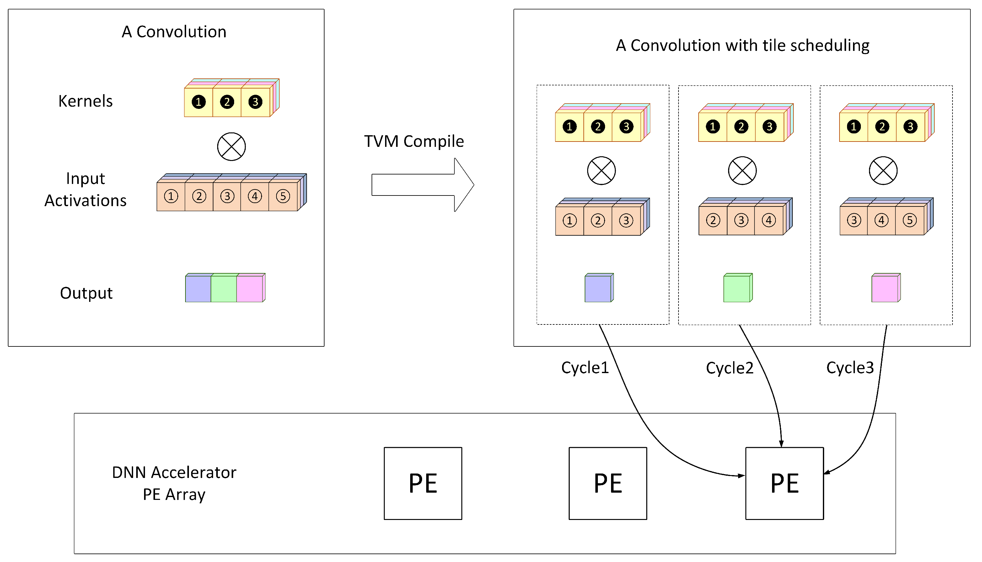
The proposed approach is based on TVM. From Figure 5, we see that when a model is input into TVM, the parser transforms it into relay IR modules. Each module comprises a series of operations supported by TVM, with every operation represented using an abstract syntax tree (AST) structure. TVM then applies a series of optimization passes over the entire tree to enhance performance. In our proposed approach, we concentrate on the stage from the frontend to the relay IR modules, with a focus on the graph level. Using the AST structure and the optimization passes in TVM, we implement a combination of model partitioning and layer fusion to achieve efficient model transformation and optimization.
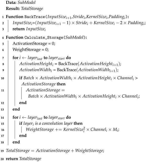
Given a sub-model executed on a PE, it is essential to calculate the storage space required by that PE. Notably, due to layer fusion, a sub-model may consist of a single layer or a set of fused layers. Additionally, with model partitioning considered, a sub-model may represent a partitioned single layer or a partitioned set of fused layers. Algorithm 1 computes the storage space needed to execute a sub-model on a PE. The input is a sub-model, and the output is the storage space required by a PE to execute the sub-model.
In the first line of Algorithm 1, we define a BackTrace function. This function uses the input dimension of the current layer, together with the stride, kernel size, and padding of the preceding layer, to compute the input dimension that the preceding layer must have to produce the output required by the current layer. The notations S t r i d e i , K e r n e l S i z e i , P a d d i n g i denote the stride, kernel size, and padding of layer i. The formula used by this function to calculate the input dimension of the preceding layer can be derived from the equations given in the literature [51].
We use the LeNet model as an example to illustrate the concept of function BackTrace in Algorithm 1. The LeNet model consists of five layers in total, with a batch size of 1. The input size of the fifth layer is (16, 5, 5), which implies that the output size of the fourth layer is also (16, 5, 5). In the fourth layer, both the stride and kernel size are (2, 2), and the padding is set to 0. Given this information, the function BackTrace can be used to compute that the height and width of the input activation to the fourth layer are both ( 5 1 ) × 2 + 2 2 × 0 = 8 + 2 = 10 .
Algorithm 1: Calculate The Required Storage Space of a Sub-Model
Electronics 14 02352 i001
   In Algorithm 1, we use the function Calculate_Storage to compute the required storage space. The variable ActivationStorage represents the storage size required for input activations. The variable WeightStorage represents the storage size required for the weights. The variable TotalStorage represents the total storage size, which includes both input activations and weights. The notation C h a n n e l _ i represents the number of channels in the layer i.
For a given sub-model, starting from the output feature map of its last layer, denoted as l a y e r l a s t , we apply the function BackTrace to traverse the network layer by layer and calculate the storage needed for the input activations of each layer. Note that because the output of the preceding layer serves as the input to the current layer, they are able to share the same memory space. Since memory space can be shared across different layers during execution, we only need to allocate the maximum storage space required among these layers.
Finally, we compute the storage space required for the weight parameters. Unlike input activations, weights cannot be shared between layers; therefore, the weight parameters of all layers must be stored in memory. In Algorithm 1, we calculate the total weight storage by summing the storage requirements of each layer’s weight parameters. Note that M i denotes the number of kernels.
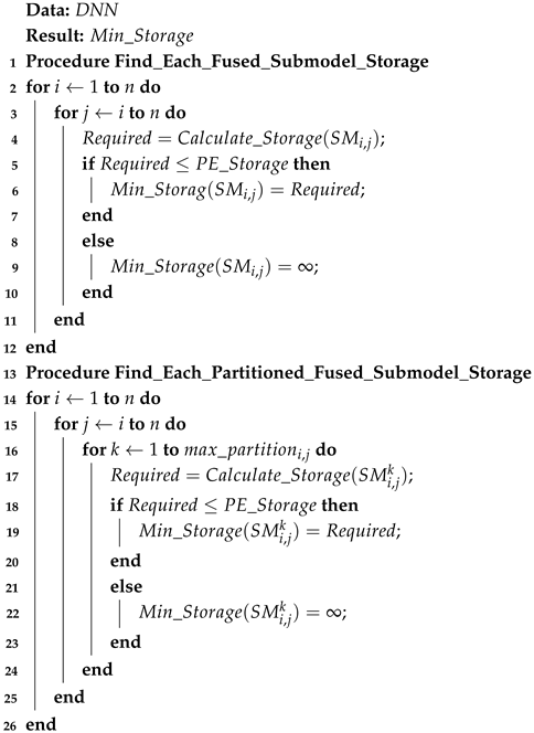
In Algorithm 2, given a DNN, our objective is to compute the minimum storage space required for every possible sub-model within the DNN. We consider two scenarios separately: one where only layer fusion is applied and another where both layer fusion and model partitioning are used.
  • Only Layer Fusion: If a DNN has n layers, there are n 1 potential points at which layer fusion can be applied. The total number of candidate solutions is given by the following equation:
    i = 0 n 1 n 1 i = 2 n 1
    A layer, or a fused layer, is referred to as a sub-model. Each candidate solution is composed of sub-models. Procedure F i n d _ E a c h _ F u s e d _ S u b m o d e l _ S t o r a g e identifies the storage required for each possible sub-model. The notation S M i , j represents a sub-model formed by applying layer fusion from layer i to layer j. We use the C a l c u l a t e _ S t o r a g e procedure from Algorithm 1 to compute the minimum storage space required for each sub-model S M i , j . The notation P E _ S t o r a g e denotes the storage space available to each PE. The notation R e q u i r e d denotes the required storage size. If the minimum storage space required by a sub-model exceeds the storage capacity provided by a PE, we consider the storage requirement of that sub-model to be infinite (i.e., the sub-model is not selected for use).
  • Layer Fusion and Model Partitioning: Considering model partitioning, we use the notation m a x _ p a r t i t i o n i , j to denote the maximum number of allowable partitions for sub-model S M i , j , a parameter that can be specified by the user. Under this constraint, the procedure F i n d _ E a c h _ P a r t i t i o n e d _ F u s e d _ S u b m o d e l _ S t o r a g e evaluates the storage requirements for all feasible combinations of layer fusion and model partitioning strategies. Within this procedure, we use the notation S M i , j k to represent a partition of sub-model S M i , j when it is divided into k partitions.
If a DNN has n layers, then in the case of layer fusion only, each candidate solution contains at most n sub-models. Suppose that the maximum number of allowable partitions for each sub-model is t, where t is a constant. Therefore, when model partitioning is applied, a candidate solution originally derived from layer fusion may lead to O( t n ) candidate solutions. Since layer fusion alone can generate 2 n 1 candidate solutions, combining layer fusion and model partitioning results in O( 2 n 1 × t n ) candidate solutions. Because t is a constant, the total number of candidate solutions in the combined approach can be expressed as O( 2 2 n 1 ). Note that the run time of the proposed approach scales proportionally with the number of candidate solutions.
Dividing a sub-model into multiple sub-models allows those partitions to run concurrently. However, the DNN accelerator must have a sufficient number of PEs to support simultaneous execution. Therefore, for each sub-model, the maximum allowable number of partitions can be set equal to the number of PEs in the accelerator.
Algorithm 2: Compute The Minimum Storage Space Required for Possible Sub-Models
Electronics 14 02352 i002
Algorithm 2 computes the minimum storage space required for all possible sub-models, where each partition resulting from model partitioning is also considered a sub-model. The computed results are stored in a database called M i n _ S t o r a g e , enabling efficient retrieval of the required storage space for any sub-model S M via the query M i n _ S t o r a g e ( S M ) .
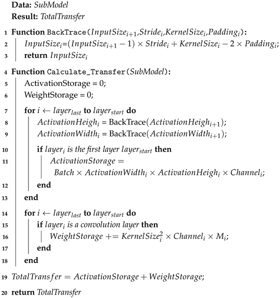
Algorithm 1 mainly calculates the storage space required for a sub-model. If we want to calculate the data transfer required for a sub-model instead, this algorithm needs to be slightly modified. To compute the data transfer for a sub-model, for input activations, we only need to consider the input activations required by the first layer, i.e., l a y e r s t a r t . The input activations for the subsequent layers do not require data transfer (because they are shared internally within the PE memory). Algorithm 3 is the algorithm used to calculate the data transfer required for a sub-model. In Algorithm 3, the variable TotalTransfer represents the total amount of data transfer, including both input activations and weights.
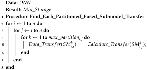
Similarly, we compute the data transfer required for all possible sub-models, treating each partition generated through model partitioning as an individual sub-model. The computed results are stored in a database, called Data_Transfer, enabling efficient retrieval of the required data transfer for any given sub-model SM via the query Data_Transfer(SM). Algorithm 4, which is a slight modification of Algorithm 2, describes the method for computing the data transfer required for all possible sub-models.
Algorithm 3: Calculate The Required Total Data Transfer of a Sub-Model
Electronics 14 02352 i003
Algorithm 4: Compute The Data Transfer Required for Possible Sub-Models
Electronics 14 02352 i004
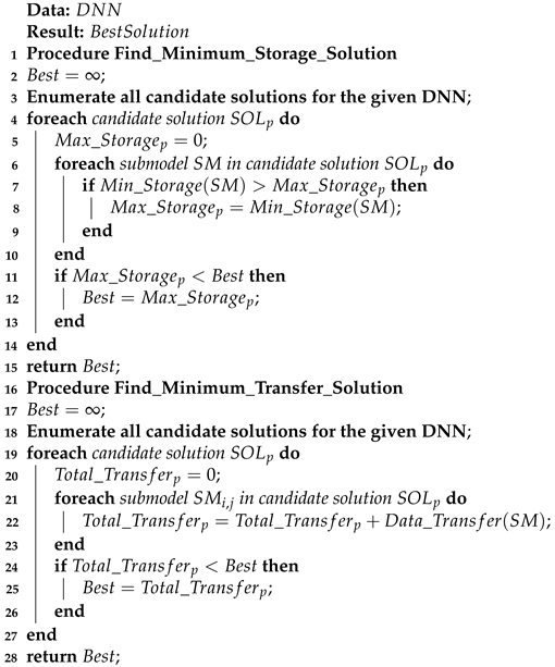
   Algorithm 5 aims to determine the optimal solution for the simultaneous application of layer fusion and model partitioning to a given DNN. To support different design objectives, we provide two distinct procedures: one that minimizes the storage space required for executing the DNN (that is, procedure F i n d _ M i n i m u m _ S t o r a g e _ S o l u t i o n ) and another that minimizes the amount of data transfer during execution (that is, procedure F i n d _ M i n i m u m _ T r a n s f e r _ S o l u t i o n ). For a given DNN, all candidate solutions arising from the joint application of layer fusion and model partitioning can be exhaustively enumerated. The two procedures in Algorithm 5 carry out an exhaustive search over the design space to identify the optimal solution based on their respective optimization objectives. The notation M a x _ S t o r a g e p denotes the maximum memory storage required among all sub-models in the candidate solution S O L p . The notation T o t a l _ T r a n s f e r p denotes the total amount of data transferred among all sub-models in the candidate solution S O L p . The notation B e s t refers to the optimal solution.
Algorithm 5: Determine the Optimal Solution for the Execution of a DNN
Electronics 14 02352 i005
The procedure F i n d _ M i n i m u m _ S t o r a g e _ S o l u t i o n is formulated to identify the minimum storage solution. For each candidate solution, this procedure first derives all associated sub-models and then determines the storage space required for each. The storage requirement of a candidate solution is defined as the maximum storage demand among its sub-models. The candidate exhibiting the lowest storage requirement is selected as the optimal solution.
The procedure F i n d _ M i n i m u m _ T r a n s f e r _ S o l u t i o n is designed to identify the solution that minimizes data transfer. For each candidate solution, this procedure first derives all associated sub-models and then calculates the data transfer required for each. The total data transfer of a candidate solution is defined as the sum of the data transfer requirements across all its sub-models. The candidate solution with the lowest total data transfer is selected as the optimal solution.
Note that in Algorithm 5, we utilize the database M i n S t o r a g e , constructed by Algorithm 2, and the database D a t a T r a n s f e r , constructed by Algorithm 4. For any sub-model S M , the query M i n _ S t o r a g e ( S M ) returns its corresponding storage space requirement. Using this database, users can invoke the procedure F i n d _ M i n i m u m _ S t o r a g e S o l u t i o n to obtain the minimum storage solution. Similarly, for any sub-model S M , the query D a t a _ T r a n s f e r ( S M ) returns its corresponding data transfer requirement. Using this database, users can invoke the procedure F i n d _ M i n i m u m _ T r a n s f e r _ S o l u t i o n to identify the minimum data transfer solution.

5. Experimental Results

In our experiments, we use the ReRAM-based DNN accelerator framework proposed in [48] as the underlying hardware architecture and evaluated our method in a variety of DNN models. The experimental evaluation comprises three main components. First, we applied our algorithm, which integrates layer fusion with model partitioning, to various models to examine its overall impact. Second, we conducted a focused analysis using the VGG-8 model to assess the algorithm’s effectiveness in minimizing data transfer under different memory size constraints. Third, we employ a larger DNN, ResNet-50, to evaluate the feasibility of applying our approach to large-scale networks.

5.1. Evaluation of Our Proposed Algorithm

In the first experiment, we use three neural network models for evaluation: LeNet (Table 1), AlexNet (Table 2), and VGG-8 (Table 3). Note that VGG-8 is a truncated version of VGG-16. The format of the input dimension is (C, H, W), where C represents the number of channels, H denotes the height (in pixels), and W denotes the width (in pixels). In a convolution layer, the format of the weight dimensions is (M, C, R, S), where M is the number of output channels, C is the number of input channels, R denotes the height (in pixels), and S denotes the width (in pixels). In a pooling layer, the kernel size is typically represented by the dimensions (R, S), where R denotes the height (in pixels) and S denotes the width (in pixels).
As shown in Table 1, LeNet consists of three convolutional layers, with an input feature map size of (1, 32, 32). The input is a grayscale image, hence the single input channel. The model reaches a maximum of 120 channels, and all convolutional kernels have a size of 5 × 5, with down sampling applied after two pooling layers. Table 2 and Table 3 present the architectures of AlexNet and VGG-8, respectively. Compared to LeNet, both models exhibit an increased number of convolutional layers (five in total), and their input feature map sizes expand to (3, 227, 227) for AlexNet and (2, 224, 224) for VGG-8. In addition, the depths of the kernel channels are significantly higher, leading to more computationally intensive processing.
Table 4, Table 5 and Table 6 present the results of our approach applied to three DNNs under different optimization scenarios. The Fused Group column in these tables indicates groups of fused layers, labeled for clarity with identifiers such as Merge1, Merge2, and so forth. The notation # A c t . refers to the data size (in bytes) associated with input activations and # W e i g h t s refers to the data size (in bytes) of the weights. When the objective is to minimize the memory space required by a PE, we first apply layer fusion and model partitioning to achieve the smallest possible memory storage space. Next, under that minimum memory storage constraint, we further reduce the data transfer volume. Taking AlexNet as an example (see Table 2), it consists of eight layers in total. Because the minimum storage requirement for Merge3 is 1,327,488 bytes (i.e., 384 + 1,327,104), we fuse the first four layers into Merge1, ensuring that memory usage remains below the Merge3 threshold. On the other hand, if the sole objective is to minimize data transfer without limiting memory space, we can fuse all layers so that all operations run on-chip at once, although at the cost of a larger memory storage space requirement.
In Table 7, we compare three methods: the conventional approach (without layer fusion or model partitioning), the layer fusion approach (with layer fusion but without model partitioning), and the proposed approach (which combines layer fusion and model partitioning). The comparison focuses on two metrics, storage space requirements and data transfer volume, across three DNN models. Note that in Table 7, the reduction rate is reported relative to the conventional approach, which serves as the baseline for comparison.
In the conventional approach, the computation of each layer involves transferring the data to the DNN accelerator for processing and then transferring them back, resulting in a high data transfer overhead. The layer fusion approach reduces the amount of data transfer by combining multiple layers into a single computation pipeline. However, this benefit comes at the cost of increased memory usage within the DNN accelerator. For example, in the case of AlexNet, the required on-chip memory increases by 65.5%.
The proposed approach addresses this trade-off by introducing model partitioning along with layer fusion. While model partitioning introduces some additional data transfers due to the parallel execution of sub-operations, it significantly reduces the memory footprint imposed by layer fusion. Moreover, model partitioning enables parallel computation, which enhances overall computational efficiency.

5.2. Impact of Storage Size Constraints on Model Partitioning

Figure 10 and Figure 11 show the amount of data transfer for the VGG-8 model under varying storage space constraints, optimized using the proposed algorithm. In Figure 10, storage space constraints are represented in units of 10 × 10 3 . As storage capacity increases, the proposed algorithm generally achieves greater reductions in data transfer. However, due to limitations in the DNN architecture and data flow structure, small increases in available storage may not always lead to immediate improvements. This is evident in the range of 370 × 10 3 to 390 × 10 3 , where data transfer remains unchanged. Overall, as the storage space increases from 390 × 10 3 to 400 × 10 3 , the total data transfer is reduced by approximately 3.2%, demonstrating the algorithm’s effectiveness in optimizing data movement under constrained storage.
In Figure 11, it is evident that significant reductions in data transfer occur within storage ranges of 390 × 10 3 to 400 × 10 3 , 800 × 10 3 to 900 × 10 3 , and 900 × 10 3 to 1000 × 10 3 . These observed trends provide valuable information for on-chip storage planning, offering guidance on how to balance performance optimization with constraints on area and power consumption.
Table 8 summarizes the storage usage of the VGG-8 model after optimization by the proposed algorithm under on-chip storage size constraints ranging from 300 × 10 3 to 1000 × 10 3 . Here, the row Peak denotes the maximum occupancy of the chip buffer during the inference process, and the row Utilization is defined as the ratio of this maximum usage to the total available storage. The results show that our memory utilization exceeds 97% in all cases. This shows that the proposed optimization strategy maintains extremely high on-chip buffer efficiency across a wide range of storage budgets, fully exploiting available hardware resources.

5.3. Analysis of Applying the Proposed Method to Larger DNNs

To evaluate the feasibility of our approach on large-scale networks, we apply it to a deeper DNN, ResNet-50. Our experiments show that exhaustively enumerating all possible combinations of layer fusion and model partitioning results in an exponential increase in the search space. The associated computation time could be extended for several years, making it impractical for real-world engineering workflows. To manage this complexity, we restrict layer fusion to convolution and max pooling layers and limit the partitioning to 36 carefully selected configurations. Because the solution space is still large, we randomly sample 10 7 candidate solutions from the solution space and choose the best. Consequently, the overall run time is reduced to approximately 24 min (running on Intel Xeon Silver 4110 CPU).
We compare our method with other model optimization strategies, and the results are summarized in Table 9. Here we compare four strategies: the conventional approach, which applies neither layer fusion nor model partitioning; the layer fusion approach, which applies layer fusion but not model partitioning; the model partitioning approach, which applies model partitioning but not layer fusion; and the proposed approach, which combines both layer fusion and model partitioning. Note that both AutoTVM [49] and Ansor [50] adopt a concept similar to the model partitioning approach but do not incorporate layer fusion in their approaches.
As shown in Table 9, pure layer fusion significantly reduces data transfer by 80.0% but increases the storage requirement to 3.9 times the original size. In contrast, pure model partitioning substantially reduces the storage footprint but does not improve data transfer. Our approach combines the advantages of both strategies. It maintains the data transfer efficiency of cross-layer fusion while using partitioning to reduce memory usage. As a result, it achieves an 80.9% reduction in maximum on-chip storage and a 77.5% reduction in data transfer, providing an optimal balance between communication cost and memory usage.
Finally, we evaluate the inference latency of the ResNet-50 model (input size 224 × 224, batch size = 1) on the ReRAM-based platform proposed in [48], comparing the baseline and our optimized version. Without any fusion or partitioning, the baseline model requires approximately 95 ms for end-to-end inference. After applying our proposed algorithm, the latency is reduced to approximately 53 ms, achieving a 1.79× speedup. This latency measurement includes both the data transfer time and the computation time, clearly demonstrating the effectiveness of our method in improving the execution efficiency of ResNet-50 on the ReRAM accelerator [48].

6. Conclusions

This paper presents a deep learning compiler based on the TVM framework for ReRAM-based DNN accelerators. The key contribution of our work is an algorithm that integrates the benefits of both layer fusion and model partitioning to optimize data storage utilization. This algorithm is seamlessly integrated into TVM to support the efficient deployment of DNN models. We evaluated our approach using three neural networks, LeNet, AlexNet, and VGG-8, under various optimization goals and hardware configurations. The experimental results demonstrate the practical effectiveness of our algorithm. Our future work aims to generalize our approach and evaluate it across a broader range of accelerators, thereby ensuring it is not restricted to ReRAM-based accelerators.

Author Contributions

Conceptualization, investigation, methodology, and validation, H.-Y.K. and L.-Y.S.; formal analysis and writing—original draft preparation: H.-Y.K., L.-Y.S. and S.-H.H.; writing—review and editing, L.-Y.S., S.-H.H. and W.-K.C.; supervision, S.-H.H. and W.-K.C. All authors have read and agreed to the published version of the manuscript.

Funding

This work was supported in part by the National Science and Technology Council, Taiwan, under grant number 110-2218-E-033-003 and grant number 112-2221-E-033-050-MY3.

Data Availability Statement

The original contributions presented in this study are included in the article. Further inquiries can be directed to the corresponding author.

Conflicts of Interest

The authors declare no conflict of interest.

References

  1. Lecun, Y.; Bottou, L.; Bengio, Y.; Haffner, P. Gradient-based learning applied to document recognition. Proc. IEEE 1998, 86, 2278–2324. [Google Scholar] [CrossRef]
  2. Krizhevsky, A.; Sutskever, I.; Hinton, G.E. ImageNet classification with deep convolutional neural networks. Commun. Acm 2017, 60, 84–90. [Google Scholar] [CrossRef]
  3. Simonyan, K.; Zisserman, A. Very deep convolutional networks for large-scale image recognition. arXiv 2014, arXiv:1409.1556. [Google Scholar]
  4. Szegedy, C.; Liu, W.; Jia, Y.; Sermanet, P.; Reed, S.; Anguelov, D.; Erhan, D.; Vanhoucke, V.; Rabinovich, A. Going deeper with convolutions. In Proceedings of the IEEE Conference on Computer Vision and Pattern Recognition, Boston, MA, USA, 7–12 June 2015; pp. 1–9. [Google Scholar]
  5. He, K.; Zhang, X.; Ren, S.; Sun, J. Deep Residual Learning for Image Recognition. In Proceedings of the 2016 IEEE Conference on Computer Vision and Pattern Recognition (CVPR), Las Vegas, NV, USA, 27–30 June 2016; pp. 770–778. [Google Scholar] [CrossRef]
  6. Iandola, F.N.; Han, S.; Moskewicz, M.W.; Ashraf, K.; Dally, W.J.; Keutzer, K. SqueezeNet: AlexNet-level accuracy with 50x fewer parameters and <0.5 MB model size. arXiv 2016, arXiv:1602.07360. [Google Scholar]
  7. Huang, G.; Liu, Z.; Maaten, L.V.D.; Weinberger, K.Q. Densely Connected Convolutional Networks. In Proceedings of the 2017 IEEE Conference on Computer Vision and Pattern Recognition (CVPR), Honolulu, HI, USA, 21–26 July 2017; pp. 2261–2269. [Google Scholar] [CrossRef]
  8. Paszke, A.; Gross, S.; Massa, F.; Lerer, A.; Bradbury, J.; Chanan, G.; Killeen, T.; Lin, Z.; Gimelshein, N.; Antiga, L.; et al. PyTorch: An Imperative Style, High-Performance Deep Learning Library. In Proceedings of the 33rd International Conference on Neural Information Processing Systems, Vancouver, BC, Canada, 8–14 December 2019; Curran Associates Inc.: Red Hook, NY, USA, 2019. [Google Scholar]
  9. Abadi, M.; Barham, P.; Chen, J.; Chen, Z.; Davis, A.; Dean, J.; Devin, M.; Ghemawat, S.; Irving, G.; Isard, M.; et al. TensorFlow: A System for Large-Scale Machine Learning. In Proceedings of the 12th USENIX Conference on Operating Systems Design and Implementation, Savannah, GA, USA, 2–4 November 2016; pp. 265–283. [Google Scholar]
  10. Chen, T.; Li, M.; Li, Y.; Lin, M.; Wang, N.; Wang, M.; Xiao, T.; Xu, B.; Zhang, C.; Zhang, Z. MXNet: A Flexible and Efficient Machine Learning Library for Heterogeneous Distributed Systems. arXiv 2015, arXiv:1512.01274. [Google Scholar]
  11. Jia, Y.; Shelhamer, E.; Donahue, J.; Karayev, S.; Long, J.; Girshick, R.; Guadarrama, S.; Darrell, T. Caffe: Convolutional architecture for fast feature embedding. In Proceedings of the 22nd ACM International Conference on Multimedia, Orlando, FL, USA, 3–7 November 2014; pp. 675–678. [Google Scholar]
  12. Jouppi, N.P.; Young, C.; Patil, N.; Patterson, D.; Agrawal, G.; Bajwa, R.; Bates, S.; Bhatia, S.; Boden, N.; Borchers, A.; et al. In-Datacenter Performance Analysis of a Tensor Processing Unit. In Proceedings of the 44th Annual International Symposium on Computer Architecture, New York, NY, USA, 24–28 June 2017; pp. 1–12. [Google Scholar] [CrossRef]
  13. Kirkpatrick, S.; Gelatt, C.D.; Vecchi, M.P. Optimization by Simulated Annealing. Science 1983, 220, 671–680. [Google Scholar] [CrossRef]
  14. Marino, R.; Kirkpatrick, S. Hard optimization problems have soft edges. Sci. Rep. 2023, 13, 3671. [Google Scholar] [CrossRef]
  15. Liu, S.; Du, Z.; Tao, J.; Han, D.; Luo, T.; Xie, Y.; Chen, Y.; Chen, T. Cambricon: An Instruction Set Architecture for Neural Networks. In Proceedings of the 2016 ACM/IEEE 43rd Annual International Symposium on Computer Architecture (ISCA), Seoul, Republic of Korea, 18–22 June 2016; pp. 393–405. [Google Scholar] [CrossRef]
  16. Jia, Z.; Tillman, B.; Maggioni, M.; Scarpazza, D.P. Dissecting the graphcore ipu architecture via microbenchmarking. arXiv 2019, arXiv:1912.03413. [Google Scholar]
  17. Rotem, N.; Fix, J.; Abdulrasool, S.; Catron, G.; Deng, S.; Dzhabarov, R.; Gibson, N.; Hegeman, J.; Lele, M.; Levenstein, R.; et al. Glow: Graph lowering compiler techniques for neural networks. arXiv 2018, arXiv:1805.00907. [Google Scholar]
  18. Cyphers, S.; Bansal, A.K.; Bhiwandiwalla, A.; Bobba, J.; Brookhart, M.; Chakraborty, A.; Constable, W.; Convey, C.; Cook, L.; Kanawi, O.; et al. Intel ngraph: An intermediate representation, compiler, and executor for deep learning. arXiv 2018, arXiv:1801.08058. [Google Scholar]
  19. Chen, T.; Moreau, T.; Jiang, Z.; Zheng, L.; Yan, E.; Cowan, M.; Shen, H.; Wang, L.; Hu, Y.; Ceze, L.; et al. TVM: An automated end-to-end optimizing compiler for deep learning. In Proceedings of the 13th USENIX Conference on Operating Systems Design and Implementation, Carlsbad, CA, USA, 8–10 October 2018; pp. 579–594. [Google Scholar]
  20. Lattner, C.; Adve, V. LLVM: A compilation framework for lifelong program analysis & transformation. In Proceedings of the International Symposium on Code Generation and Optimization, San Jose, CA, USA, 20–24 March 2004; pp. 75–86. [Google Scholar] [CrossRef]
  21. Lu, W.; Yan, G.; Li, J.; Gong, S.; Han, Y.; Li, X. FlexFlow: A Flexible Dataflow Accelerator Architecture for Convolutional Neural Networks. In Proceedings of the 2017 IEEE International Symposium on High Performance Computer Architecture (HPCA), Austin, TX, USA, 4–8 February 2017; pp. 553–564. [Google Scholar] [CrossRef]
  22. Wang, Y.; Wang, Y.; Li, H.; Shi, C.; Li, X. Systolic Cube: A Spatial 3D CNN Accelerator Architecture for Low Power Video Analysis. In Proceedings of the 56th Annual Design Automation Conference 2019, Las Vegas, NV, USA, 2–6 June 2019; pp. 1–6. [Google Scholar] [CrossRef]
  23. Du, Z.; Fasthuber, R.; Chen, T.; Ienne, P.; Li, L.; Luo, T.; Feng, X.; Chen, Y.; Temam, O. Shidiannao: Shifting Vision Processing Closer to the Sensor. In Proceedings of the 2015 ACM/IEEE 42nd Annual International Symposium on Computer Architecture (ISCA), Portland, OR, USA, 13–17 June 2015; Volume 43, pp. 92–104. [Google Scholar] [CrossRef]
  24. Chen, Y.H.; Emer, J.; Sze, V. Eyeriss: A Spatial Architecture for Energy-Efficient Dataflow for Convolutional Neural Networks. In Proceedings of the 2016 ACM/IEEE 43rd Annual International Symposium on Computer Architecture (ISCA), Seoul, Republic of Korea, 18–22 June 2016; Volume 44, pp. 367–379. [Google Scholar] [CrossRef]
  25. Chen, Y.H.; Krishna, T.; Emer, J.S.; Sze, V. Eyeriss: An Energy-Efficient Reconfigurable Accelerator for Deep Convolutional Neural Networks. IEEE J. Solid-State Circuits 2017, 52, 127–138. [Google Scholar] [CrossRef]
  26. Chen, Y.H.; Yang, T.J.; Emer, J.; Sze, V. Eyeriss v2: A Flexible Accelerator for Emerging Deep Neural Networks on Mobile Devices. IEEE J. Emerg. Sel. Top. Circuits Syst. 2019, 9, 292–308. [Google Scholar] [CrossRef]
  27. Kwon, H.; Samajdar, A.; Krishna, T. MAERI: Enabling Flexible Dataflow Mapping over DNN Accelerators via Reconfigurable Interconnects. ACM Sigplan Not. 2018, 53, 461–475. [Google Scholar] [CrossRef]
  28. Kao, H.Y.; Chen, X.J.; Huang, S.H. Convolver Design and Convolve-Accumulate Unit Design for Low-Power Edge Computing. Sensors 2021, 21, 5081. [Google Scholar] [CrossRef] [PubMed]
  29. Weng, Y.K.; Huang, S.H.; Kao, H.Y. Block-Based Compression and Corresponding Hardware Circuits for Sparse Activations. Sensors 2021, 21, 7468. [Google Scholar] [CrossRef]
  30. Weng, Y.K.; Huang, S.H.; Kao, H.Y. Block-Based Compression for Reducing Indexing Cost of DNN Accelerators. In Proceedings of the 2021 IEEE International Conference on Consumer Electronics-Taiwan (ICCE-TW), Penghu, Taiwan, 15–17 September 2021; pp. 1–2. [Google Scholar]
  31. Chang, C.H.; Kao, H.Y.; Huang, S.H. Hardware implementation for multiple activation functions. In Proceedings of the 2019 IEEE International Conference on Consumer Electronics-Taiwan (ICCE-TW), Yilan, Taiwan, 20–22 May 2019; pp. 1–2. [Google Scholar]
  32. Zhao, Y.; Chen, X.; Wang, Y.; Li, C.; You, H.; Fu, Y.; Xie, Y.; Wang, Z.; Lin, Y. SmartExchange: Trading Higher-cost Memory Storage/Access for Lower-cost Computation. In Proceedings of the 2020 ACM/IEEE 47th Annual International Symposium on Computer Architecture (ISCA), Valencia, Spain, 30 May–3 June 2020; pp. 954–967. [Google Scholar] [CrossRef]
  33. Chatarasi, P.; Kwon, H.; Raina, N.; Malik, S.; Haridas, V.; Parashar, A.; Pellauer, M.; Krishna, T.; Sarkar, V. Marvel: A Data-centric Compiler for DNN Operators on Spatial Accelerators. arXiv 2020, arXiv:2002.07752. [Google Scholar]
  34. Kwon, H.; Chatarasi, P.; Pellauer, M.; Parashar, A.; Sarkar, V.; Krishna, T. Understanding Reuse, Performance, and Hardware Cost of DNN Dataflows: A Data-Centric Approach Using MAESTRO. arXiv 2020, arXiv:1805.02566. [Google Scholar]
  35. Lin, W.H.; Kao, H.Y.; Huang, S.H. A Design Framework for Hardware Approximation of Deep Neural Networks. In Proceedings of the 2019 International Symposium on Intelligent Signal Processing and Communication Systems (ISPACS), Taipei, Taiwan, 3–6 December 2019; pp. 1–2. [Google Scholar]
  36. Lin, W.H.; Kao, H.Y.; Huang, S.H. Hybrid Dynamic Fixed Point Quantization Methodology for AI Accelerators. In Proceedings of the 2021 18th International SoC Design Conference (ISOCC), Jeju Island, Republic of Korea, 6–9 October 2021; pp. 282–283. [Google Scholar]
  37. Liu, F.; Zhao, W.; Wang, Z.; Chen, Y.; Liang, X.; Jiang, L. ERA-BS: Boosting the Efficiency of ReRAM-Based PIM Accelerator with Fine-Grained Bit-Level Sparsity. IEEE Trans. Comput. 2024, 73, 2320–2334. [Google Scholar] [CrossRef]
  38. Chen, W.; Qi, Z.; Akhtar, Z.; Siddique, K. Resistive-RAM-Based In-Memory Computing for Neural Network: A Review. Electronics 2022, 11, 3667. [Google Scholar] [CrossRef]
  39. Shafiee, A.; Nag, A.; Muralimanohar, N.; Balasubramonian, R.; Strachan, J.P.; Hu, M.; Williams, R.S.; Srikumar, V. ISAAC: A Convolutional Neural Network Accelerator with In-Situ Analog Arithmetic in Crossbars. In Proceedings of the 2016 ACM/IEEE 43rd Annual International Symposium on Computer Architecture (ISCA), Seoul, Republic of Korea, 18–22 June 2016; Volume 44, pp. 14–26. [Google Scholar] [CrossRef]
  40. Chi, P.; Li, S.; Xu, C.; Zhang, T.; Zhao, J.; Liu, Y.; Wang, Y.; Xie, Y. PRIME: A Novel Processing-in-Memory Architecture for Neural Network Computation in ReRAM-Based Main Memory. In Proceedings of the 2016 ACM/IEEE 43rd Annual International Symposium on Computer Architecture (ISCA), Seoul, Republic of Korea, 18–22 June 2016; Volume 44, pp. 27–39. [Google Scholar] [CrossRef]
  41. Wong, H.S.P.; Lee, H.Y.; Yu, S.; Chen, Y.S.; Wu, Y.; Chen, P.S.; Lee, B.; Chen, F.T.; Tsai, M.J. Metal–Oxide RRAM. Proc. IEEE 2012, 100, 1951–1970. [Google Scholar] [CrossRef]
  42. Park, J. Neuromorphic Computing Using Emerging Synaptic Devices: A Retrospective Summary and an Outlook. Electronics 2020, 9, 1414. [Google Scholar] [CrossRef]
  43. Mittal, S. A Survey of ReRAM-Based Architectures for Processing-In-Memory and Neural Networks. Mach. Learn. Knowl. Extr. 2018, 1, 5. [Google Scholar] [CrossRef]
  44. Kaur, R.; Asad, A.; Mohammadi, F. A Comprehensive Review of Processing-in-Memory Architectures for Deep Neural Networks. Computers 2024, 13, 174. [Google Scholar] [CrossRef]
  45. Ankit, A.; Hajj, I.E.; Chalamalasetti, S.R.; Ndu, G.; Foltin, M.; Williams, R.S.; Faraboschi, P.; Hwu, W.-m.W.; Strachan, J.P.; Roy, K.; et al. PUMA: A Programmable Ultra-efficient Memristor-based Accelerator for Machine Learning Inference. In Proceedings of the Twenty-Fourth International Conference on Architectural Support for Programming Languages and Operating Systems, New York, NY, USA, 13–19 April 2019; pp. 715–731. [Google Scholar] [CrossRef]
  46. Song, L.; Qian, X.; Li, H.; Chen, Y. PipeLayer: A Pipelined ReRAM-Based Accelerator for Deep Learning. In Proceedings of the 2017 IEEE International Symposium on High Performance Computer Architecture (HPCA), Austin, TX, USA, 4–8 February 2017; pp. 541–552. [Google Scholar] [CrossRef]
  47. Peng, X.; Liu, R.; Yu, S. Optimizing Weight Mapping and Data Flow for Convolutional Neural Networks on RRAM Based Processing-In-Memory Architecture. In Proceedings of the 2019 IEEE International Symposium on Circuits and Systems (ISCAS), Sapporo, Japan, 26–29 May 2019; pp. 1–5. [Google Scholar] [CrossRef]
  48. Kao, H.Y.; Huang, S.H.; Cheng, W.K. Design Framework for ReRAM-Based DNN Accelerators with Accuracy and Hardware Evaluation. Electronics 2022, 11, 2107. [Google Scholar] [CrossRef]
  49. Chen, T.; Zheng, L.; Yan, E.; Jiang, Z.; Moreau, T.; Ceze, L.; Guestrin, C.; Krishnamurthy, A. Learning to Optimize Tensor Programs. In Proceedings of the Advances in Neural Information Processing Systems, Montréal, QC, Canada, 3–8 December 2018; Bengio, S., Wallach, H., Larochelle, H., Grauman, K., Cesa-Bianchi, N., Garnett, R., Eds.; Curran Associates, Inc.: New York, NY, USA, 2018; Volume 31. [Google Scholar]
  50. Zheng, L.; Jia, C.; Sun, M.; Wu, Z.; Yu, C.H.; Haj-Ali, A.; Wang, Y.; Yang, J.; Zhuo, D.; Sen, K.; et al. Ansor: Generating High-Performance Tensor Programs for Deep Learning. In Proceedings of the 14th USENIX Symposium on Operating Systems Design and Implementation (OSDI 20), Online, 4–6 November 2020; pp. 863–879. [Google Scholar]
  51. Krichen, M. Convolutional Neural Networks: A Survey. Computers 2023, 12, 151. [Google Scholar] [CrossRef]
Figure 1. Concept of CNN.
Electronics 14 02352 g001
Figure 2. Data flow of CIM.
Electronics 14 02352 g002
Figure 3. Data flow of CIM with multiple sub-arrays.
Electronics 14 02352 g003
Figure 4. (a) A Column of ReRAM Array. (b) ReRAM Array.
Electronics 14 02352 g004
Figure 5. The Compilation Flow of TVM.
Electronics 14 02352 g005
Figure 6. The Case That The Storage Capacity of a PE Cannot Accommodate an Entire Stage.
Electronics 14 02352 g006
Figure 7. An Illustration of Model Partitioning.
Electronics 14 02352 g007
Figure 8. The benefits of layer fusion. (a) No layer fusion is applied. (b) Layer fusion is applied.
Electronics 14 02352 g008
Figure 9. Proposed Idea for Model Partitioning on a DNN Model.
Electronics 14 02352 g009
Figure 10. Data Transfer of VGG-8 from Storage Size 300 × 10 3 to 400 × 10 3 .
Electronics 14 02352 g010
Figure 11. Data Transfer of VGG-8 from Storage Size 300 × 10 3 to 1000 × 10 3 .
Electronics 14 02352 g011
Table 1. Structure of LeNet Model.
LayerOperationInput DimensionWeight DimensionPadding DimensionStrides
1Conv ( 1 , 32 , 32 ) ( 6 , 1 , 5 , 5 ) ( 0 , 0 , 0 , 0 ) ( 1 , 1 )
2MaxPool ( 6 , 28 , 28 ) ( 2 , 2 ) ( 0 , 0 , 0 , 0 ) ( 2 , 2 )
3Conv ( 6 , 14 , 14 ) ( 16 , 6 , 5 , 5 ) ( 0 , 0 , 0 , 0 ) ( 1 , 1 )
4MaxPool ( 16 , 10 , 10 ) ( 2 , 2 ) ( 0 , 0 , 0 , 0 ) ( 2 , 2 )
5Conv ( 16 , 5 , 5 ) ( 120 , 16 , 5 , 5 ) ( 0 , 0 , 0 , 0 ) ( 1 , 1 )
6out ( 120 , 1 , 1 ) N/AN/AN/A
Table 2. Structure of AlexNet Model.
LayerOperationInput DimensionWeight DimensionPadding DimensionStrides
1Conv ( 3 , 227 , 227 ) ( 96 , 3 , 11 , 11 ) ( 0 , 0 , 0 , 0 ) ( 4 , 4 )
2MaxPool ( 96 , 55 , 55 ) ( 3 , 3 ) ( 0 , 0 , 0 , 0 ) ( 2 , 2 )
3Conv ( 96 , 27 , 27 ) ( 256 , 96 , 5 , 5 ) ( 2 , 2 , 2 , 2 ) ( 1 , 1 )
4MaxPool ( 256 , 27 , 27 ) ( 3 , 3 ) ( 0 , 0 , 0 , 0 ) ( 2 , 2 )
5Conv ( 256 , 13 , 13 ) ( 384 , 256 , 3 , 3 ) ( 1 , 1 , 1 , 1 ) ( 1 , 1 )
6Conv ( 384 , 13 , 13 ) ( 384 , 384 , 3 , 3 ) ( 1 , 1 , 1 , 1 ) ( 1 , 1 )
7Conv ( 384 , 13 , 13 ) ( 256 , 384 , 3 , 3 ) ( 1 , 1 , 1 , 1 ) ( 1 , 1 )
8MaxPool ( 256 , 13 , 13 ) ( 3 , 3 ) ( 0 , 0 , 0 , 0 ) ( 2 , 2 )
9out ( 256 , 6 , 6 ) N/AN/AN/A
Table 3. Structure of VGG-8 Model.
LayerOperationInput DimensionWeight DimensionPadding DimensionStrides
1Conv ( 3 , 224 , 224 ) ( 64 , 3 , 3 , 3 ) ( 1 , 1 , 1 , 1 ) ( 1 , 1 )
2Conv ( 64 , 224 , 224 ) ( 64 , 64 , 3 , 3 ) ( 1 , 1 , 1 , 1 ) ( 1 , 1 )
3MaxPool ( 64 , 224 , 224 ) ( 2 , 2 ) ( 0 , 0 , 0 , 0 ) ( 2 , 2 )
4Conv ( 64 , 112 , 112 ) ( 128 , 64 , 3 , 3 ) ( 1 , 1 , 1 , 1 ) ( 1 , 1 )
5Conv ( 128 , 112 , 112 ) ( 128 , 128 , 3 , 3 ) ( 1 , 1 , 1 , 1 ) ( 1 , 1 )
6MaxPool ( 128 , 112 , 112 ) ( 2 , 2 ) ( 0 , 0 , 0 , 0 ) ( 2 , 2 )
7Conv ( 128 , 56 , 56 ) ( 256 , 128 , 3 , 3 ) ( 1 , 1 , 1 , 1 ) ( 1 , 1 )
8out ( 256 , 56 , 56 ) N/AN/AN/A
Table 4. LeNet Results with Varying Optimization Goals.
Minimize StorageMinimize Transfer
Fused GroupLayer#Act./per Partition#Weights/per PartitionFused GroupLayer#Act.#Weights
Merge1Conv8642550Merge1Conv470450,550
MaxPoolMaxPool
ConvConv
MaxPoolMaxPool
Merge2Conv40048,000Conv
Table 5. AlexNet Results with Varying Optimization Goals.
Minimize StorageMinimize Transfer
Fused GroupLayer#Act./per Partition#Weights/per PartitionFused GroupLayer#Act.#Weights
Merge1Conv4704626,016Merge1Conv290,4003,745,824
MaxPoolMaxPool
ConvConv
MaxPoolMaxPool
Merge2Conv256884,736Conv
Merge3Conv3841,327,104Conv
Merge4Conv3456884,736Conv
MaxpoolMaxpool
Table 6. VGG-8 Results with Varying Optimization Goals.
Minimize StorageMinimize Transfer
Fused GroupLayer#Act./per Partition#Weights/per PartitionFused GroupLayer#Act.#Weights
Merge1Conv1024259,776Merge1Conv3,211,264554,688
ConvConv
MaxPoolMaxPool
ConvConv
ConvConv
MaxPoolMaxPool
Merge2Conv1152294,912Conv
Table 7. Evaluation of Diverse Optimization Methods.
Storage SizeData TransferStorage Size Reduction RateData Transfer Reduction Rate
LeNetConventional48,40073,070N/AN/A
Layer Fusion55,25455,374−12.4%32.0%
Ours48,40067,4540.0%8.3%
AlexNetConventional1,392,0005,436,283N/AN/A
Layer Fusion4,036,2244,045,440−65.5%34.4%
Ours1,327,4884,955,6484.9%9.7%
VGG8Conventional3,248,12823,127,744N/AN/A
Layer Fusion3,765,9524,512,448−13.8%412.5%
Ours296,0648,273,088997.1%179.6%
Table 8. Memory Storage Utilization under Varying On-Chip Storage Size Constraints.
Constraint ( × 10 3 bytes)3004005006007008009001000
Peak ( × 10 3 bytes)300396.75498596680797.69893.69981.69
Utilization (%)10099.1899.6099.3397.1499.7199.3098.17
Table 9. Comparison of different strategies (using Resnet50).
ApproachStorage SizeData TransferStorage Size
Reduction Rate
Data Transfer
Reduction Rate
Conventional106,954,7521,215,675,025N/AN/A
Layer Fusion411,041,792243,986,432−285.9%80.0%
Model Partitioning4,202,4961,215,678,86596.1%0.0%
Ours20,455,424273,371,90480.9%77.5%
Disclaimer/Publisher’s Note: The statements, opinions and data contained in all publications are solely those of the individual author(s) and contributor(s) and not of MDPI and/or the editor(s). MDPI and/or the editor(s) disclaim responsibility for any injury to people or property resulting from any ideas, methods, instructions or products referred to in the content.

