Article

Backpack Client Selection Keeping Swarm Learning in Industrial Digital Twins for Wireless Mapping

School of Software, Henan University of Science and Technology, Luoyang 471023, China
*
Author to whom correspondence should be addressed.
Electronics 2025, 14(12), 2323; https://doi.org/10.3390/electronics14122323
Submission received: 25 April 2025 / Revised: 25 May 2025 / Accepted: 3 June 2025 / Published: 6 June 2025

Abstract

:
Digital twin virtual–real mapping and precise modeling require the synchronization of large amounts of data, which leads to high communication overhead in wireless channels in industrial Internet of Things (IoT). To solve this problem, this study proposes an architecture of Digital Twin–Swarm learning (DT-SL) for industrial IoT digital twins. SL is an emerging distributed federated learning (FL) method that eliminates the need for centralized servers completely. However, it faces the problem of wireless channel congestion caused by high concurrent parameter transmission. In view of the above architecture, a novel KSL scheme based on the backpack model is used to construct the DT model. The backpack optimization problem is used to select the client with the largest contribution to participate in Keeping SL twin modeling. In addition, the experimental results evaluated the performance of the proposed method. The absolute value of the client’s updated parameter quantity decreased by 23.6% on average. The convergence rate of the aggregation model increased by 34.1%, and the model aggregation MSE value decreased to 0.03.

Graphical Abstract

1. Introduction

This is regarded as a revolutionary architecture to improve production efficiency in the information age in the industrial IoT, especially in the context of Industry 4.0 [1]. Factory production edge deployment includes DT with wireless mobile edge computing capabilities, which is an edge-side technology [2,3]. DT effectively connects the device layer and the network layer. It collects operational and environmental data and adapts the state control of physical entities, which provides an excellent solution for the intelligent allocation of industrial production line resources [3,4,5].
DT industrial IoT relies heavily on large amounts of multisource heterogeneous data collected from different swarms of devices, thus forming data silos. The secure sharing of data across multiple production lines and logistics channels is another key challenge of DT industrial IoT [6,7]. To solve these problems, SL came into being, which is a fully decentralized FL method that achieves a perfect balance between massive data and privacy in industrial IoT. SL was originally proposed to integrate the privacy of medical data. It is completely independent of central server coordination and satisfies the requirement that data owners do not provide original data for model training [8,9]. The trained model parameters are shared on the wireless swarm network and aggregated into the global model. The aggregated model is sent to the local device to continue participating in the next training stage until the model converges [10].
SL is a special type of FL that uses high-concurrency transmission of model parameters on a recurrent network. The transmission reduces the timeliness of communication in models with high real-time requirements, such as DT, and increases wireless mapping errors [11]. Much scholars’ research on FL is limited to a simplified wireless communication channel model. The gradient parameter transmission is secure but faces the problem of high communication overhead [12,13]. Some scholars have proposed gradient sparsification and quantification methods; however, for the DT industrial IoT architecture, it is difficult to adapt to the needs of real-time and accurate mapping [14,15]. Meanwhile, there is currently little research on the combination of SL and industrial IoT. Moreover, the original SL scheme does not implement the screening of client devices.
The backpack model is a classic combinatorial optimization method that is often used to select a group of objects with the greatest benefits under resource constraints (such as communication bandwidth, energy consumption, etc.). In the industrial IoT scenarios, physical devices are considered items. Their contribution represents value. The communication volume required for parameter upload represents weight, and the communication capacity is set as backpack capacity. By solving the backpack optimization problem, devices with the greatest contribution can be selected to participate in the Keeping SL twin modeling and update parameters without exceeding the communication threshold.
Therefore, in response to the above-mentioned wireless mapping timeliness problem of industrial DT, the contributions of this article include the following:
(1)
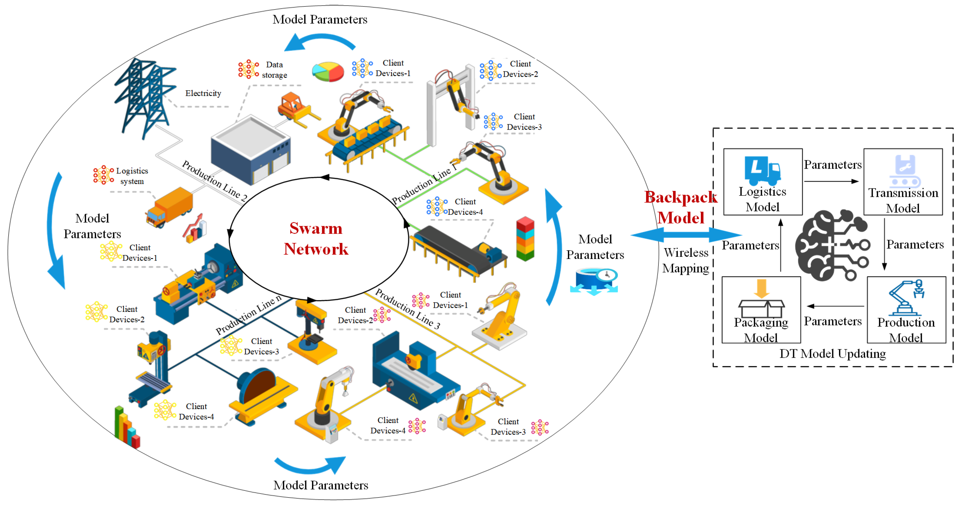
We designed a DT-driven industrial IoT SL architecture, in which DT technology realizes dynamic perception in complex industrial IoT environments, and SL enhances the interconnection between heterogeneous devices and production lines.
(2)
Based on DT-SL, we propose a novel KSL scheme based on the backpack model to construct the DT model. Moreover, we select clients with greater contributions to complete wireless mapping and Keeping SL twin modeling to optimize the wireless channel transmission rate.
(3)
Compared with the existing methods, the timeliness and convergence rate of the proposed method are improved.

2. Related Work

2.1. Digital Twins in Industrial IoT

Digital twins are integrated with real-time industrial IoT data to establish comprehensive mappings of equipment and production lines for multisource scenarios, through which industrial production efficiency is enhanced. In [16], a multi-tier industrial DT architecture was constructed, comprising a client layer, an edge layer, and a twin layer. The edge servers continuously update the twin states, including the operational status, historical data, and behavioral models, which improves the execution accuracy of industrial production. An industrial IoT architecture that combines federated learning with DT was proposed in [17], where the twin layer was implemented through lightweight edge servers. The local update coefficients and model compression ratios were adaptively adjusted to achieve real-time precise mapping. Developed on the multi-tier industrial DT architecture in [18], client interaction statuses were analytically modeled, and an efficient communication method for multi-device distributed computing was introduced. Moreover, reference [19] enhanced partial model updating efficiency by incorporating DAG-based block sharding technology into industrial DT architectures, through which edge-enabled industrial twin models were established. Building on equipment operational parameters and interaction states, an asynchronous weighted strategy for global model updating was presented in [20] to optimize resource allocation. Additionally, a geometry–physics behavior-rule multidimensional model fusion methodology was adopted in [2] for developing high-fidelity virtual workshop models, enabling the effective deployment of DT technologies in industrial IoT scenarios.

2.2. Client Selection in Distributed Learning

The computational capabilities of heterogeneous devices in industrial IoT networks are constrained by their resource disparities. Devices with low computing efficiency prolong global model training cycles, thereby degrading convergence rates. To address this issue, a client selection algorithm constrained by time thresholds is proposed in [21], where participating clients are selected through evaluating heterogeneous training durations. In [22], a stratified sampling strategy is introduced to select quasi-static clients within uniform time intervals, minimizing client dropout and communication cycles. Building on this framework, Ref. [23] categorizes clients into hierarchical tiers based on training time windows, ensuring in-tier selections while preventing cross-layer synchronization delays. A dynamic adaptive scheduling method is developed in [24], which determines optimal per-round time cutoffs by analyzing historical convergence patterns to identify the most suitable clients in distributed networks. Similarly, Ref. [25] enhances client selection by prioritizing devices with high-quality data weights within predefined baselines. However, this method creates imbalanced selection criteria, resulting in suboptimal gradient aggregation and coarse-grained model accuracy.
Ref. [26] introduces a client selection strategy that minimizes variance across time scales, prioritizing clients with high availability for training contrasting time-based methods. Ref. [27] employs a chunked incremental learning method to precisely schedule and match client training tasks based on gradient aggregation patterns. Ref. [28] proposes a client selection algorithm using model-parameter-sharing block fading values and local gradient norms, combined with resource allocation, to efficiently schedule low-configuration devices. Ref. [29] develops a balanced scheduling strategy for clients operating in both high- and low-SNR environments, ensuring the usability of the selected devices. Ref. [30] optimizes bandwidth allocation for model parameter transmission through energy-efficient client selection, enabling precise multidimensional client selection.
These methods rely on device availability, computational resources, and energy assessments for client selection. However, they crudely estimate device contributions to model convergence and fail to address redundant data in selected clients, leading to inefficient high-volume parameter transmission without significant accuracy improvements.

3. System Model

There is a typical industrial IoT production environment that includes equipment clusters such as production lines, packaging lines, and logistics lines. A large amount of heterogeneous mechanical equipment and multi-type sensors (temperature, pressure, speed, etc.) in each industrial production line regularly collect operating data perception information, as shown in Figure 1.
A DT-driven industrial IoT SL architecture is designed to realize dynamic perception in complex industrial IoT environments. Based on DT-SL, we propose a novel KSL-scheme-based backpack model to construct the DT model. We select clients with greater contributions to complete wireless mapping and Keeping SL twin modeling to optimize the wireless channel transmission rate.
We provide the meaning and source of the key variables in the article formula, as shown in Table 1. We assume that each device i performs model training on the local dataset D i = { ( x j , y j ) } j = 1 n i . The training goal is to minimize the local loss function and optimize the model parameters of a single device. For the regression problem of device clusters, the loss function of a single device is defined as follows:
L i ( θ i ) = 1 n i j = 1 n i ( f ( x j ; θ i ) y j ) 2
where f ( x j ; θ i ) is the classification prediction of device i for input sample x j , y j belongs to the true sample label, and n i is the number of samples in device i .
L i ( θ i ) = 1 n i j = 1 n i k = 1 C y j k log ( p j k )
where p j k is the predicted probability of a single device i for sample j belonging to category k ; C is the number of categories in the device production line; and y j k is the label of sample j corresponding to category k .
In SL, the gradient descent algorithm is used for optimization. A single device i updates the model parameter θ i , and the formula is expressed as:
θ i ( t + 1 ) = θ i ( t ) η L i ( θ i ( t ) )
where η is the learning rate and L i ( θ i ( t ) ) is the gradient of the loss function for device i at iteration t . It is a discrete optimization formula that uses the iteration as the update unit. For the mean squared error loss function, the gradient is calculated as:
L i ( θ i ) = 2 n i j = 1 n i ( f ( x j ; θ i ) y j ) f ( x j ; θ i )
where f ( x j ; θ i ) is the gradient of model f ( x j ; θ i ) with respect to parameter θ i . The gradient of the cross-entropy loss function is calculated as:
L i ( θ i ) = 1 n i j = 1 n i k = 1 C y j k p j k p j k
where p j k is the gradient of the model output probability p j k , with respect to the model parameter θ i .

4. Client Selection and Backpack Model

In industrial scenarios, limited computing resources select a swarm of devices S { 1 , 2 , , N } , so that the total contribution of the devices is maximized. The total interactive communication parameter of the model is less than or equal to the set maximum threshold B max . The objective function and constraints of the backpack model are expressed as:
maximize i = 1 N c i x i
i = 1 N b i x i B max
where N is the total number of devices participating in SL in the industrial production line S . The modeling of device i in the swarm network is represented by 1, and the non-modeling is represented by 0, x i { 0 , 1 } . c i is the contribution of device i , and b i is the parameter quantity of the model uploaded by the device. The model gradually calculates the optimal solution under different communication cost constraints. We define D P [ k ] as the dynamic programming state, where each entry represents the maximum contribution achievable under a communication budget range [ 0 , k ] . The state transfer equation is expressed as:
D P   [ k ] = max ( D P   [ k ] , D P   [ k b i ] + c i )     s . t .   k b i
We performed initial calculations on the backpack model. We assume that no equipment in the production line is selected to participate in wireless interaction and build a twin model, where all D P [ k ] = 0 , as follows:
D P   [ 0 ] = 0 , k [ 0 , B max ]
where, based on the contribution of industrial production equipment c i and the parameter update transmission volume b i , the optimal solution for calculating the capacity of a single backpack k is:
D P   [ B max ] = max ( D P   [ B max ] ,   D P   [ k b i ]   +   c i )
The maximum contribution can be obtained by selecting the optimal solution (backpack capacity) of the client’s device to satisfy 0 k B max . When the selected device completes the local model training and updates the client, the device will upload the updated model parameters θ i ( t + 1 ) to the SL network architecture. The weighted average update of the SL network node model is:
θ ( t + 1 ) = i = 1 N w i θ i ( t + 1 )
where θ ( t + 1 ) is the global model generated by aggregating the local model updates of all selected clients; w i is the weight of device i ; and θ i ( t + 1 ) is the model parameter of device i after local training in the t + 1 th round. The threshold is set according to the computing power of the device.

4.1. Convergence Proof

For the local training of each device, the goal is to minimize the loss function L i ( θ i ) . We assume that L i ( θ i ) is a continuous differentiable convex function that satisfies smoothness. Smoothness guarantees stable gradient updates. Convexity ensures the existence of a unique global optimum and allows for the derivation of linear convergence rates under appropriate learning rates, as follows:
  L i ( θ 1 ) L i ( θ 2 ) L θ 1 θ 2 , θ 1 , θ 2
where Formula (12) indicates that the gradient of the loss function is Lipschitz continuous. Constant L is the Lipschitz constant. The loss function L i ( θ i ) has strong convexity. There exists a constant μ , such that:
L i ( θ 2 ) L i ( θ 1 ) + L i ( θ 1 ) ( θ 2 θ 1 ) + μ 2 θ 2 θ 1 2 , θ 1 , θ 2
where μ is a strong convexity constant, which limits the curvature of the loss function. We let the local model parameter be θ i ( t ) . The global optimal solution is θ i * and the error is θ i ( t ) θ i * . Based on Formulae (12) and (13), we update Formula (3). We expand the square of the error as follows:
  θ i ( t + 1 ) θ i * 2 = θ i ( t ) θ i * 2 2 η L i ( θ i ( t ) ) θ i ( t ) θ i * 2 + η 2 L i ( θ i ( t ) ) 2
The algorithm applies the strong convexity shown in Formula (13) and the Lipschitz continuity in Formula (12), and θ 1 = θ i * , θ 2 = θ i ( t ) . Because L i ( θ i * ) = 0 , we can get the following two inequalities:
L i ( θ i ( t ) θ i * ) ( θ i ( t ) θ i * ) μ θ i ( t ) θ i * 2
  L i ( θ i ( t ) ) 2 L 2 θ i ( t ) θ i * 2
We substitute the above two inequalities into the square error expression (14) as follows:
  θ i ( t + 1 ) θ i * 2 1 2 η μ + η 2 L 2 θ i ( t ) θ i * 2
We choose a learning rate 0 < η μ L 2 . Moreover, because 1 2 η μ + η 2 L 2 1 η μ , we know that the gradient descent error satisfies:
  θ i ( t + 1 ) θ i * 2 ( 1 η μ ) θ i ( t ) θ i * 2
where 1 η μ < 1 ensures that the model error gradually decreases and has linear convergence. The convergence of the SL network node model satisfies:
θ ( t + 1 ) = i S w i θ i ( t + 1 )
In the device set selected by Formula (10), the model update of each device satisfies the local convergence assumption. We let the global optimal solution be θ * and the global error be θ ( t ) θ * . We expand the global error and take the square of the norm as follows:
  θ ( t + 1 ) θ * 2 = i S w i θ i ( t + 1 ) θ * 2
The algorithm uses Cauchy–Schwarz inequality. Assuming that the data between the devices are independent, the covariance term approaches zero:
  θ ( t + 1 ) θ * 2 i S w i 2   θ i ( t + 1 ) θ * 2 + i j w i w j ( θ i ( t + 1 ) θ * ) ( θ j ( t + 1 ) θ * )   θ ( t + 1 ) θ * 2 i S w i 2   θ i ( t + 1 ) θ * 2 + σ 2
We substitute Formula (14) into the above formula and get:
  θ ( t + 1 ) θ * 2 ( 1 η μ ) i S w i 2   θ i ( t ) θ * 2 + σ 2
Due to i S w i = 1 , w i 1 | S | , and i S w i 2 1 | S | , we perform variance normalization and variance simplification, as follows:
θ ( t + 1 ) θ * 2 ( 1 η μ )   θ ( t ) θ * 2 + σ 2 | S |
where σ 2 is the local data distribution variance. It extends the local convergence of Equation (14) to the global model, which shows the influence of the variance of the SL network nodes and σ 2 on the convergence speed. The more nodes in the SL network, the faster the convergence rate of the global model.

4.2. Computational Complexity

The communication parameter quantity constraint for the SL network training is k = 0 , 1 , , B max . N devices update D P [ k ] . The time complexity of dynamic programming is calculated as O ( N · B max ) . The space complexity calculation is for the B max device to store an array D P : O ( B max ) . Meanwhile, the process of dynamically selecting a subset of device clients that meet the constraints to participate in training to improve communication efficiency is shown in Algorithm 1.
Algorithm 1: Backpack-Swarm Learning in DT
1. Input: local dataset D i = { ( x j , y j ) } j = 1 n i , number of local rounds t , number of global rounds T , local learning rate η , initialization parameters θ i .
2. for  t = 0,1 , , T  do
3. dataset D i from to i client:
4.     L i ( θ i ) = 1 n i j = 1 n i k = 1 C y j k log ( p j k )
5.   for local training θ i in i  do
6    if client i is to satisfy: i = 1 N b i x i B m a x and D P [ k ]
7.     model update θ i t + 1 θ i :
               θ i t + 1 = θ i t η L i θ i t
8.       else select client i training:
9.        θ t + 1 = i S w i θ i t + 1
10.   end for
11.  end for
12. Output:  θ t + 1 : updating each node of the swarm

5. Numerical Results

This section contains our experimental setup and analysis. The experiments were conducted on a hardware system equipped with an Intel(R) Core (TM) i7-13700F CPU and NVIDIA RTX4070Ti super 16G GPU (The manufacturers of the CPU and GPU are Intel Corporation and NVIDIA Corporation, respectively. Both manufacturers are located in Santa Clara, CA, USA). The simulation was implemented using PyTorch (CUDA 11.8) to build a distributed training platform. The GPU and CPU communication was facilitated using PCI-E 4.0.
We use two typical datasets (MNIST and CIFAR10), which contain different data types and diverse categories, respectively, as shown in Table 2. The typical baseline methods FedAvg [7], SL [9], DDT-CSL [10], and the KSL-DT are compared and evaluated in three aspects. FedAvg is a classic federated learning method that aggregates the local model parameters through a central server to update the global model. SL is an advanced fully decentralized federated learning method that improves privacy and robustness. DDT-CSL builds twins to perceive the status of physical devices in real time and dynamically optimize resource allocation, which significantly improves the real-time performance and communication efficiency in industrial IoT. KSL-DT selects clients with greater contributions to complete wireless mapping and Keeping SL twin modeling to optimize the wireless channel transmission rate.

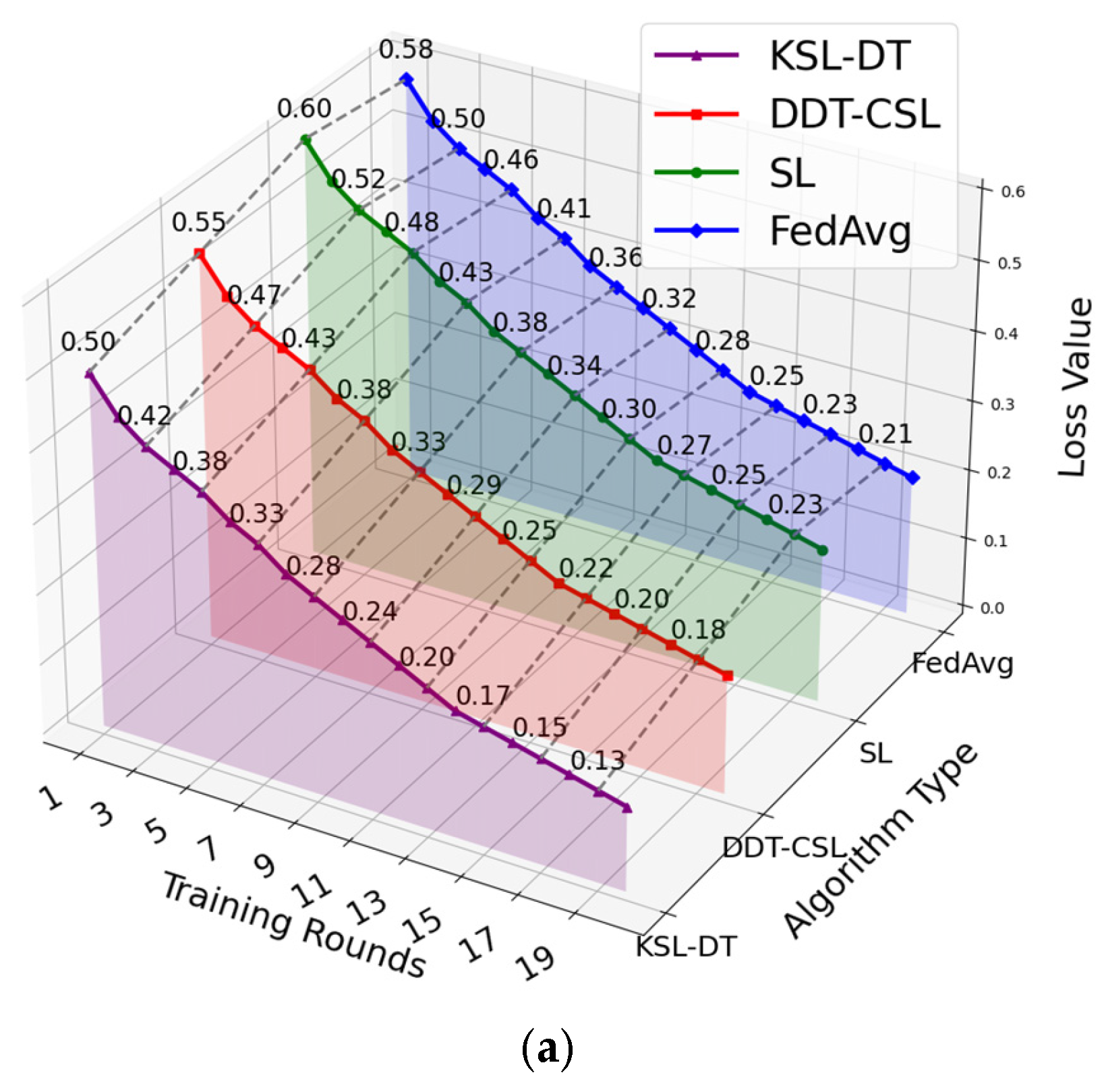
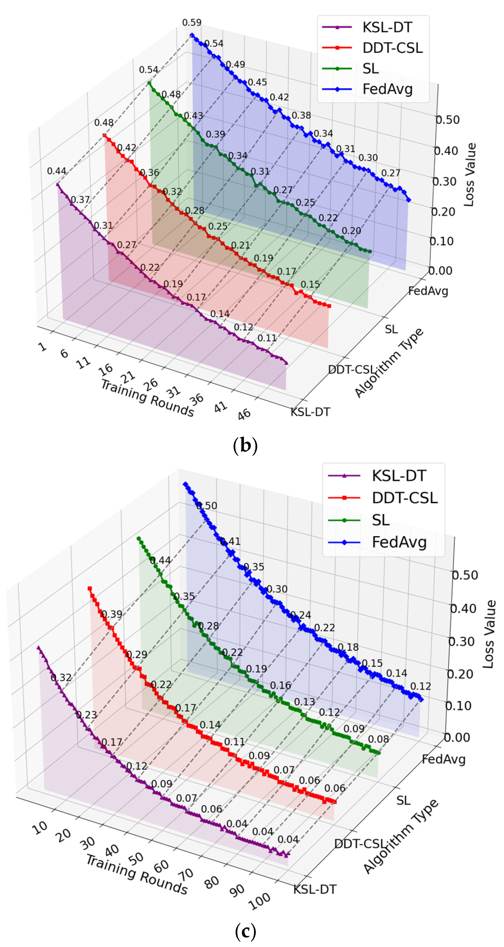
5.1. Convergence Rate of the Model

We selected the loss value change trend of four baselines on the MNIST dataset (grayscale images), which was used to evaluate the convergence rate and model fit of the model. The experimental results are shown in Figure 2. As shown in Figure 2a, during initial training, the loss value ranged from 0.5 to 0.6, and all four algorithms showed a relatively stable downward trend. Compared with the other three algorithms, the loss values of KSL-DT in the 20th round were reduced by 0.05, 0.1, and 0.08, respectively. The convergence rate of the KSL-DT model selection in the first 20 rounds of aggregate training was not significantly better than that of the other three baseline algorithms. As shown in Figure 2b, in the first 50 rounds of training, the average loss values of the four algorithms were 0.234, 0.283, 0.343, and 0.409, respectivley. KSL-DT showed the lowest average loss value. As shown in Figure 2c, when gradually increasing the number of training rounds to 100, KSL-DT generally shows the fastest and deepest descent in the experiment, which is significantly better than that of SL and FedAvg. The loss value of the curve approaches 0.04. From the qualitative analysis of the observation results, we found that KSL-DT has the fastest convergence rate, as shown in Figure 2c, compared to DDT-CSL. The curve area is the smallest and the slope of the loss curve is the largest. In addition, the algorithm proposed in this study has the best convergence rate compared with the other three methods and improves by 34.1%. This is because each selected client (the client in the backpack) uploads the local update (gradient parameter) to the SL architecture to achieve wireless mapping Φ :
G k , i ( t ) = Φ ( θ k , i ( t + 1 ) , Parameter   distribution )
where auxiliary information contains the gradient parameter distribution of the local model. In the DT environment (cooperative node), the model parameters in the swarm network are updated and deeply integrated G k , i ( t ) , denoted as Ω :
θ ( t + 1 ) = Ω ( { G k , i ( t ) } )
KSL-DT introduces the fast virtual iteration provided by “DT” and the multi-model complementary characteristics brought by “Backpack SL.” It promotes the non-independent closure of the local model training in the swarm network. The global aggregation model is no longer limited to the average weight update. The complex transformation of Φ ( · ) and Ω ( · ) is used in the DT structure to realize the modeling of the SL network.

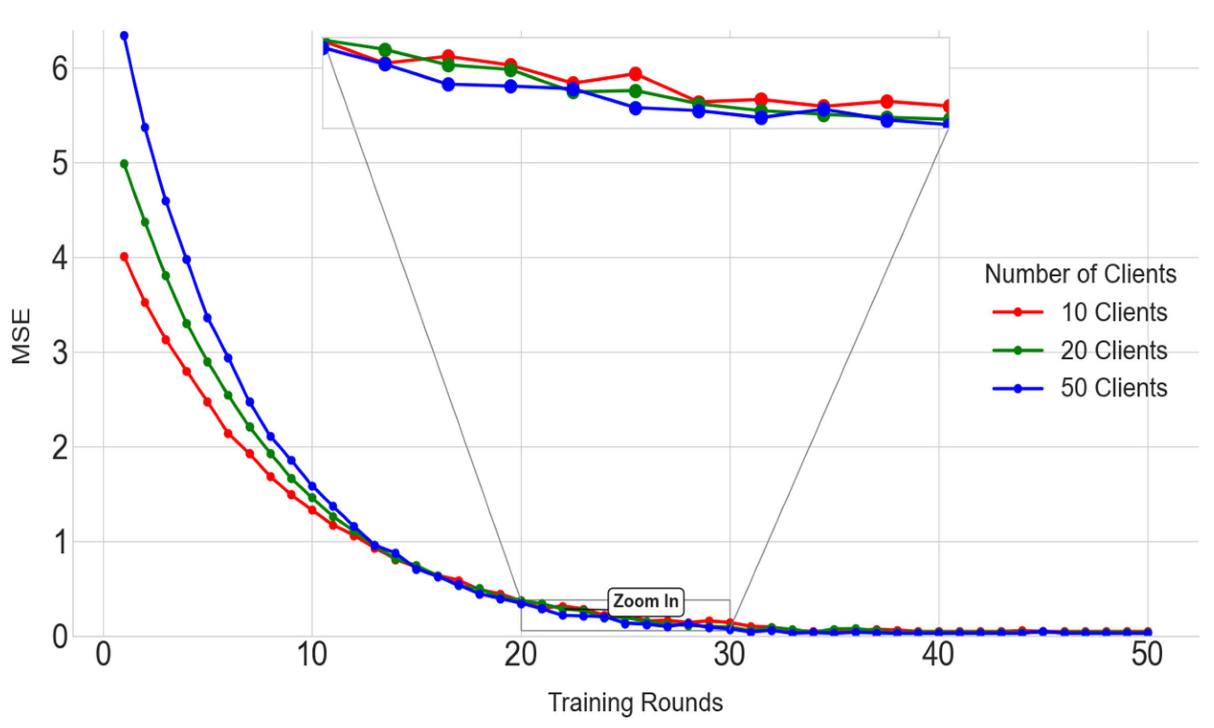
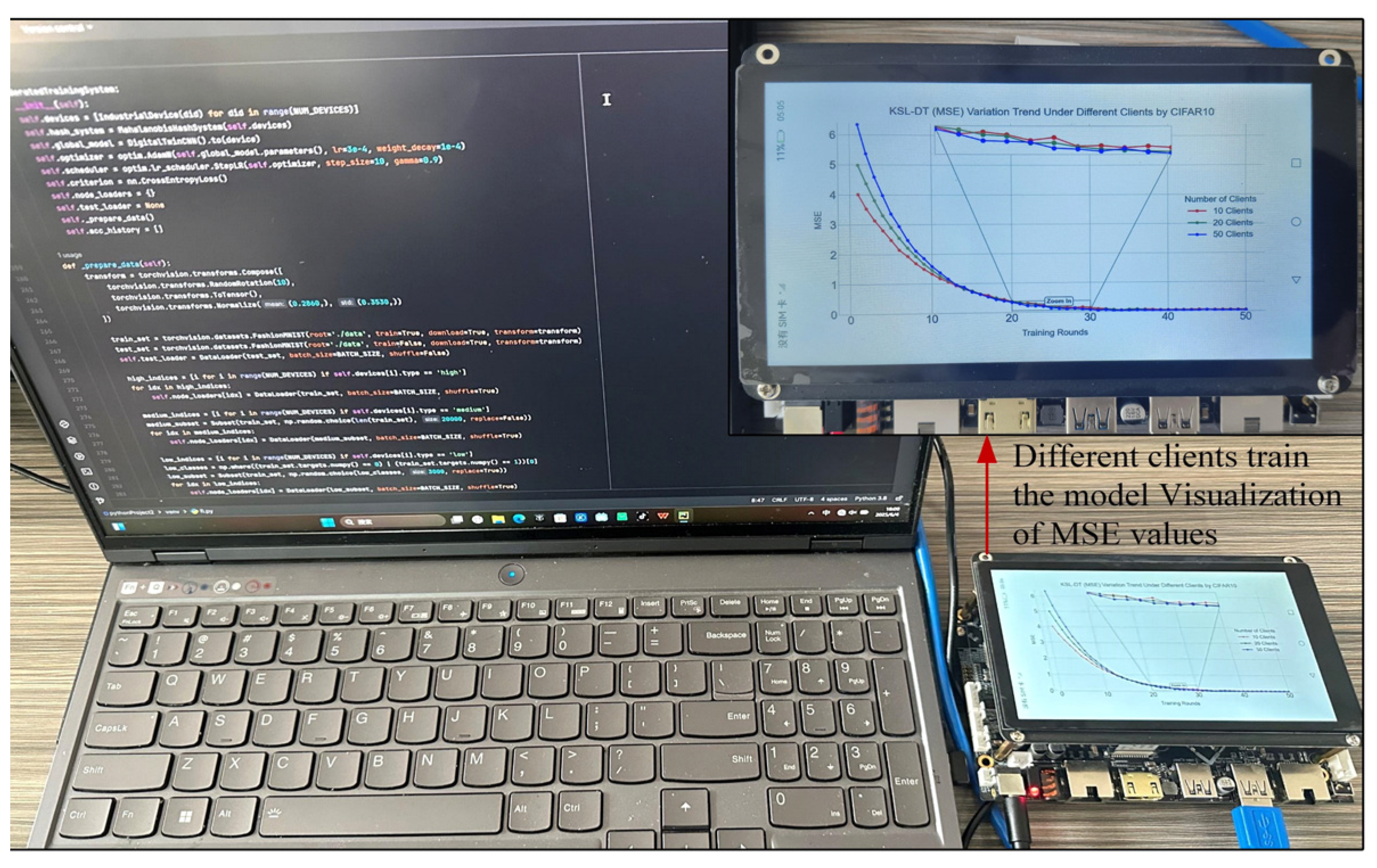
5.2. Model MSE Value Verification

On the basis of Experiment A, after we choose CIFAR10 of the RGB image type to verify the backpack model client selection, KSL-DT updates the model’s MSE value. Based on the backpack model client selection method, we, respectively, select the number of clients with the largest contribution value. The number of clients included the following: 10, 20, and 50, as shown in Figure 3. In the initial training phase of the model, the coordinated update of the swarm network nodes was not sufficient, which resulted in a higher initial MSE. (The initial MSE for 10 clients is about 4.02, while the MSE for 20 and 50 clients in rounds 0 to 1 is 4.99 and 6.35, respectively). As the number of selected clients gradually increases, the amount of data for each client decreases relatively. The distribution is more heterogeneous, and the contribution value is more uniform, as shown in Table 3. Between rounds 0 and 20, the MSE shows an obvious downward trend, with the MSE values for 10, 20, and 50 clients decreasing by 3.23, 4.04, and 5.36, respectively. The MSE with 50 clients has the largest decrease compared to the MSE with 10 and 20 clients. This experimentally verifies the theory of the influence of network node variance on the convergence rate in Formula (23) above. The more nodes (i.e., the number of clients) in the SL network, the faster the global model converges. In the late convergence state of the model, we observed that the result of the three types of clients was around 20 to 30 rounds, and the three curves all dropped below 1 in the Zoom In. Then, they stabilized. Between 30 and 50 rounds, the MSE value continued to slowly approach 0.05 to 0.03, which shows that the model has generalization ability in different client selections. At the same time, as the number of rounds increases, the information on different clients is integrated under the knowledge sharing mechanism Ω ( · ) of KSL-DT, and the MSE decreases rapidly. Through the parallel and complementary learning of DT and backpack models, KSL-DT can absorb the characteristics of each client more quickly and fully, which shows fast convergence and a low final error.
We compare and evaluate the different client contributions on the RGB dataset (CIFAR10) to verify the scalability of KSL-DT on the hardware (model: RK3568_HM_costdown/V03). The industrial equipment model is set up, which can be trained and mapped in real time on the mobile terminal, as shown in Figure 4, which supports the application capability of the verification model.

5.3. Parameter Transmission Amount for the Model

Based on Experiments A and B, we validated the proposed method with two types of datasets: grayscale and RGB images. We also compared the amount of model parameter transmission. In MNIST, KSL-DT reduces the amount of parameter transmission by 49.88%, 68.05%, and 78.31% compared with the other three baseline algorithms, respectivley. In CIFAR-10, KSL-DT reduces the amount of parameter transmission by 59.66%, 65.51%, and 84.60% compared with the other three baseline algorithms, respectivley. In both datasets, the amount of parameter transmission of the KSL-DT model is the smallest. This shows that KSL-DT has low communication overhead and reduces network congestion for high concurrent transmission. In terms of the difference in parameter growth, KSL-DT increases from ~40 k to ~69 k, with an absolute value of 72.5%. The other three algorithms increase from ~99 k to ~138 k, ~115 k to ~216 k, and ~258 k to ~319 k, with relative increases of 39.39%, 87.83%, and 23.6%, respectively. Among the four algorithms, the number of model training parameters of CIFAR-10 is significantly higher than that of MNIST. This is because the data structure of CIFAR-10 is complex. Moreover, it requires a deeper or wider network structure to learn the features of color images. In CIFAR-10, KSL-DT still shows the smallest amount of model parameter transmission. This shows that the proposed method has good robustness. At the same time, observing Figure 5, due to the KSL-DT proposed in this study, the representation of some key layers or knowledge distillation is synchronized on the client, which greatly reduces the amount of parameter transmission. Meanwhile, in the wireless mapping channel of the DT, a single device collaboratively calculates and directly updates the local model, which reduces the transmission of high-concurrency parameters.

6. Conclusions

To address the communication overhead caused by data-driven DT and the congestion of high-concurrency wireless channels caused by distributed FL, we propose a new KSL scheme based on the backpack model. It selects the client with the largest contribution to participate in Keeping SL twin modeling, which explicitly solves the defects of high communication overhead and slow convergence speed caused by the concurrent transmission of the model. Through experimental comparison, the robustness and convergence speed of the proposed algorithm are verified. The asynchrony problem of SL will be explored in the future.

Author Contributions

Methodology, X.W.; Software, X.W., N.S. and Y.G.; Validation, X.W.; Investigation, N.S.; Resources, X.W., N.S. and Y.G.; Data curation, X.W.; Writing—original draft, X.W.; Writing—review and editing, P.Z.; Visualization, Y.G.; Supervision, P.Z.; Project administration, X.W. and P.Z. All authors have read and agreed to the published version of the manuscript.

Funding

This work is fully supported by the Frontier Exploration Projects of Longmen Laboratory (No. LMQYTSKT034), Key Research and Development and Promotion of Special (Science and Technology) Project of Henan Province, China (No. 252102210158).

Data Availability Statement

Our datasets have been made public through DOI:10.21227/n5xv-nf18. The dataset names are as follows: Data mnist fmnist cifar10.

Conflicts of Interest

The authors declare no conflicts of interest. The funders had no role in the design of this study; in the collection, analyses, or interpretation of the data; in the writing of the manuscript; or in the decision to publish the results.

References

  1. Nguyen, D.C.; Pathirana, P.N.; Ding, M.; Seneviratne, A. Secure computation offloading in blockchain based IoT networks with deep reinforcement learning. IEEE Trans. Netw. Sci. Eng. 2021, 8, 3192–3208. [Google Scholar] [CrossRef]
  2. Tao, F.; Cheng, Y.; Cheng, J.; Zhang, M. Theory and technology of cyber physical fusion in digital twin workshop. Comput. Integr. Manuf. Syst. 2017, 23, 1603–1611. [Google Scholar]
  3. Tao, F.; Sui, F.; Liu, A.; Qi, Q.; Zhang, M.; Song, B.; Guo, Z.; Lu, S.C.-Y.; Nee, A.Y.C. Digital twin-driven product design framework. Int. J. Prod. Res. 2019, 57, 3935–3953. [Google Scholar] [CrossRef]
  4. Gehrmann, C.; Gunnarsson, M. A digital twin-based industrial automation and control system security architecture. IEEE Trans. Ind. Inform. 2020, 16, 669–680. [Google Scholar] [CrossRef]
  5. Xu, H.; Wu, J.; Pan, Q.; Guan, X.; Guizani, M. A survey on digital twin for industrial internet of things: Applications, technologies and tools. IEEE Commun. Surv. Tutor. 2023, 25, 2569–2598. [Google Scholar] [CrossRef]
  6. Qi, Q.; Tao, F.; Hu, T.; Anwer, N.; Liu, A.; Wei, Y.; Wang, L.; Nee, A. Enabling technologies and tools for digital twin. J. Manuf. Syst. 2021, 58, 3–21. [Google Scholar] [CrossRef]
  7. Yang, Z.; Zhang, X.; Wu, D.; Wang, R.; Zhang, P.; Wu, Y. Efficient asynchronous federated learning research in the internet of vehicles. IEEE Internet Things J. 2022, 10, 7737–7748. [Google Scholar] [CrossRef]
  8. Warnat-Herresthal, S.; Schultze, H.; Shastry, K.L.; Manamohan, S.; Mukherjee, S.; Garg, V.; Sarveswara, R.; Händler, K.; Pickkers, P.; Aziz, N.A.; et al. Swarm learning for decentralized and confidential clinical machine learning. Nature 2021, 594, 265–270. [Google Scholar] [CrossRef]
  9. Saldanha, O.L.; Quirke, P.; West, N.P.; James, J.A.; Loughrey, M.B.; Grabsch, H.I.; Salto-Tellez, M.; Alwers, E.; Cifci, D.; Laleh, N.G.; et al. Swarm learning for decentralized artificial intelligence in cancer histopathology. Nat. Med. 2022, 28, 1232–1239. [Google Scholar] [CrossRef]
  10. Xiang, W.; Li, J.; Zhou, Y.; Cheng, P.; Jin, J.; Yu, K. Digital twin empowered industrial IoT based on credibility-weighted swarm learning. IEEE Trans. Ind. Inform. 2024, 20, 775–784. [Google Scholar] [CrossRef]
  11. Xing, L.; Zhao, P.; Gao, J.; Wu, H.; Ma, H. A survey of the social internet of vehicles: Secure data issues, solutions, and federated learning. IEEE Intell. Transp. Syst. Mag. 2023, 15, 70–84. [Google Scholar] [CrossRef]
  12. Imteaj, A.; Thakker, U.; Wang, S.; Li, J.; Amini, M.H. A survey on federated learning for resource constrained IoT devices. IEEE Internet Things J. 2021, 9, 1–24. [Google Scholar] [CrossRef]
  13. Khan, L.U.; Saad, W.; Han, Z.; Hossain, E.; Hong, C.S. Federated learning for internet of things: Recent advances, taxonomy, and open challenges. IEEE Commun. Surv. Tutor. 2021, 23, 1759–1799. [Google Scholar] [CrossRef]
  14. Uddin, M.P.; Xiang, Y.; Lu, X.; Yearwood, J.; Gao, L. Federated learning via disentangled information bottleneck. IEEE Trans. Serv. Comput. 2022, 16, 1874–1889. [Google Scholar] [CrossRef]
  15. Wen, J.; Zhang, Z.; Lan, Y.; Cui, Z.; Cai, J.; Zhang, W. A survey on federated learning: Challenges and applications. Int. J. Mach. Learn. Cybern. 2023, 14, 513–535. [Google Scholar] [CrossRef]
  16. He, S.; Ren, T.; Jiang, X.; Xu, M. Client selection and resource allocation for federated learning in digital-twin-enabled industrial internet of things. In Proceedings of the IEEE Wireless Communications and Networking Conference (WCNC), Glasgow, UK, 26–29 March 2023; pp. 1–6. [Google Scholar]
  17. Yang, W.; Yang, Y.; Xiang, W.; Yuan, L.; Yu, K.; Alonso, Á.H.; Ureña, J.U.; Pang, Z. Adaptive optimization federated learning enabled digital twins in industrial IoT. J. Ind. Inf. Integr. 2024, 38, 100521. [Google Scholar] [CrossRef]
  18. Zhao, Y.; Li, L.; Liu, Y.; Fan, Y.; Lin, K.-Y. Communication efficient federated learning for digital twin systems of industrial internet of things. IFAC-PapersOnLine 2022, 55, 210–215. [Google Scholar] [CrossRef]
  19. Sisinni, E.; Saifullah, A.; Han, S.; Jennehag, U.; Gidlund, M. Industrial internet of things: Challenges, opportunities, and directions. IEEE Trans. Ind. Inform. 2018, 14, 4724–4734. [Google Scholar] [CrossRef]
  20. Lu, Y.; Huang, X.; Zhang, K.; Maharjan, S.; Zhang, Y. Communication-efficient federated learning for digital twin edge networks in industrial IoT. IEEE Trans. Ind. Inform. 2021, 17, 5709–5718. [Google Scholar] [CrossRef]
  21. Nishio, T.; Yonetani, R. Client selection for federated learning with heterogeneous resources in mobile edge. In Proceedings of the IEEE International Conference on Communications (ICC), Shanghai, China, 20–24 May 2019; pp. 1–7. [Google Scholar]
  22. Abdulrahman, S.; Tout, H.; Mourad, A.; Talhi, C. FedMCCS: Multicriteria client selection model for optimal IoT federated learning. IEEE Internet Things J. 2021, 8, 4723–4735. [Google Scholar] [CrossRef]
  23. Chai, Z.; Ali, A.; Zawad, S.; Yan, E.; Yan, F.; Li, Y.; Zhou, T.; Rangwala, H. Tifl: A tier-based federated learning system. In Proceedings of the 29th International Symposium on High-Performance Parallel and Distributed Computing, Stockholm, Sweden, 23–26 June 2020; pp. 125–136. [Google Scholar]
  24. Shin, J.; Li, Y.; Liu, Y.; Lee, S.-J. Fedbalancer: Data and pace control for efficient federated learning on heterogeneous clients. In Proceedings of the 20th Annual International Conference on Mobile Systems, Applications and Services, Portland, OR, USA, 27 June–1 July 2022; pp. 436–449. [Google Scholar]
  25. Lai, F.; Zhu, X.; Madhyastha, H.V.; Chowdhury, M. Oort: Efficient federated learning via guided participant selection. In USENIX Symposium on Operating Systems Design and Implementation (OSDI); {USENIX} Association: Berkeley, CA, USA, 2021. [Google Scholar]
  26. Ribero, M.; Vikalo, H.; de Veciana, G. Federated learning under intermittent client availability and time-varying communication constraints. IEEE J. Sel. Top. Signal Process. 2023, 17, 98–111. [Google Scholar] [CrossRef]
  27. Ma, H.; Guo, H.; Lau, V.K.N. Communication-efficient federated multitask learning over wireless networks. IEEE Internet Things J. 2023, 10, 609–624. [Google Scholar] [CrossRef]
  28. Amiri, M.M.; Gunduz, D.; Kulkarni, S.R.; Poor, H.V. Convergence of update aware device scheduling for federated learning at the wireless edge. IEEE Trans. Wirel. Commun. 2021, 20, 3643–3658. [Google Scholar] [CrossRef]
  29. Yang, H.H.; Liu, Z.; Quek, T.Q.S.; Poor, H.V. Scheduling policies for federated learning in wireless networks. IEEE Trans. Commun. 2020, 68, 317–333. [Google Scholar] [CrossRef]
  30. Xu, J.; Wang, H. Client selection and bandwidth allocation in wireless federated learning networks: A long-term perspective. IEEE Trans. Wirel. Commun. 2021, 20, 1188–1200. [Google Scholar] [CrossRef]
Figure 1. DT industrial IoT swarm learning model based on backpack.
Electronics 14 02323 g001
Figure 2. Loss value evaluation under the MNIST dataset ((a) Training epochs 20; (b) Training epochs 50; (c) Training epochs 100).
Electronics 14 02323 g002aElectronics 14 02323 g002b
Figure 3. MSE of the SL based on the backpack model.
Electronics 14 02323 g003
Figure 4. Real-time model training and visualization on the mobile client.
Electronics 14 02323 g004
Figure 5. Evaluation of parameter transmission amount.
Electronics 14 02323 g005
Table 1. Key variables description.
VariablesMeaningSource (Equations)
L i ( θ i ) the loss function of device i (1), (3), (12)–(16)
n i number of local dataset samples of device i (1), (2)
θ i ( t ) model parameters of device i at iteration t (3), (14)–(18), (22), (23)
L i ( θ i ( t ) ) the gradient of loss function of device i at the t th iteration(3)–(5)
w i the communication volume (i.e., weight) of device i (11), (19)–(22)
B max the system’s maximum communication overhead threshold(7), (9), (10)
μ strong convexity constant(13), (15), (17), (18), (22), (23)
σ 2 variance of local data distribution(21)–(23)
Table 2. Dataset content.
Data NameMNISTCIFAR-10
Data Typehandwritten numbersactual object image
Image Dimensions28 × 28, single channel (grayscale)32 × 32, 3 channels (RGB)
Number Of Categories10 (numbers 0 to 9)10 (airplane, bird, and so on)
Training Set Size70,00060,000
Data SourceYann LeCun websiteCIFAR website
Table 3. MSE under different client selection numbers.
Training Rounds10 Clients20 Clients50 Clients
04.024.996.35
32.503.053.84
52.012.372.96
101.561.781.89
200.790.950.99
500.050.030.03
Disclaimer/Publisher’s Note: The statements, opinions and data contained in all publications are solely those of the individual author(s) and contributor(s) and not of MDPI and/or the editor(s). MDPI and/or the editor(s) disclaim responsibility for any injury to people or property resulting from any ideas, methods, instructions or products referred to in the content.

