Towards Scientific Knowledge Graphs: Dependency Graph Analysis Using Graph Neural Networks for Extracting Scientific Relations

Abstract

Scientific relation extraction plays a crucial role in constructing scientific knowledge graphs that can contextually integrate knowledge from the scientific literature. However, a large majority of existing efforts do not support human guidance, which hinders refining the construction of scientific knowledge graphs and, thus, the natural cycle of scientific knowledge integration. Therefore, there is a necessity to ground the human–machine collaboration in learned mechanisms, the prerequisite of which is quantifying the contribution of candidate mechanisms. In addressing this, we introduce an efficient summation node architecture by leveraging a graph neural network (GNN) on semantic patterns among dependency graphs. Then, we quantify the potential of different semantic invariance in serving as semantic interfaces towards the flexible construction of scientific knowledge graphs. Specifically, we posit that collocation-level patterns can enhance both extraction accuracy and F1 scores. Our proposed solutions exhibit promising performances for certain relations under bi-classification configurations, facilitating the learning of more semantic invariance from the word level to the collocation level. In conclusion, we assert that the flexible and robust construction of scientific knowledge graphs in the future will necessitate continual improvements to augment learned semantic invariance. This can be achieved through the development of more integrated and extended input graphs and transformer-based GNN architectures.

1. Introduction

As the sheer volume of scientific publications increases, it becomes increasingly challenging to ensure comprehensive consideration and integration of all existing knowledge, leading to a narrowing of knowledge utilization [1]. In other words, knowledge cannot be effectively utilized when it is fragmented and not even noticed. To solve this problem, it is necessary to automate the process of integrating information from scientific literature to assist manual efforts in comprehensively integrating existing knowledge. To this end, a structured representation of scientific knowledge is necessary to minimize the risk of fragmentation during the accumulation of knowledge. One of the effective approaches for scientific knowledge integration is a scientific knowledge graph [2], which consists of nodes and edges. Generally, the nodes represent entities of interest, while the edges between the nodes describe the relationships between their corresponding entities [3].

Scientific relation extraction plays a crucial role in constructing knowledge graphs from text and domain knowledge graphs by linking entities. Many studies of scientific relation extraction have been performed at the sentence level, which means a pair of focused entities should co-occur within the same sentence. Past efforts have tried to train the models by directly feeding the whole input sentence into the models based on spans of words [4,5,6,7], which explored ways of organizing tokens parsed from input text into the continuous sequences (i.e., spans) and then modeling token-wise and span-wise relationships for performance optimization. Text in the input sentence was usually embedded in a contextualized way using SciBERT [8] specifically for scientific information extraction datasets or BERT [9]. Because of the special structure of attention-based embedders like BERT, tokens and spans were linked together in the attention matrices as nodes, which can be interpreted as token-wise or span-wise attention graphs. Hence, it can be summarized that the span-based methods actually adopted implicit graph designs and mainly exploits sequential patterns in the form of spans.

Compared to the implicit graph designs, there were more direct practices that explicitly performed graph modeling for scientific relation extraction. Major related efforts originated from performing multi-category classification on nodes (i.e., one node can belong to multiple topic classes) in document-level graph datasets based on citation networks such as Cora [10], Citeseer [11], and PubMed [12]. Each node in the mentioned graph datasets represents a scientific article and is described via a binary vector in which each binary value indicates the presence of a specific word. Based on the multi-category classification of documents, scientific relation classification was performed indirectly towards building a type of scientific knowledge graph with nodes representing documents and three types of edges: having exactly the same research topics, sharing partial topics, and sharing no topics. In other words, such knowledge graphs only describe bibliometric coupling relations between document-level text and, thus, are less detailed than knowledge graphs built from extracting relations within sentences.

For sentence-level scientific relation extraction, graph-based methods for the previous document-level extraction have been transferred. Existing experiments have already revealed that, for relation extraction, information from syntax graphs such as those generated by dependency parsing can be helpful when it is fused on top of pretrained representations [13]. A large proportion of graph-based work processing the syntax graphs focused on graph neural networks (GNNs), such as graph attention networks (GATs) [14] and graph convolutional networks (GCNs) [15]. The core of GNNs is the information diffusion mechanism [16] on the graph data structure. For an input graph, the basic processing units of a typical GNN correspond to nodes in the graph one-by-one and are linked in the same pattern as the input graph presents. Generally, the update of units’ states and the information exchange among them continue until reaching a stable equilibrium, after which the GNN output is computed locally at each node based on the unit state. Some work already adopted variants of graph neural networks in their designed end-to-end solution for scientific relation extraction, but there is still large potential in improving performance.

For flexible construction of scientific knowledge graphs, this work aims to quantify the potential of improving scientific relation extraction by exposing different levels of semantic invariance (i.e., invariant patterns in semantics). Scientific knowledge integration should be a sustainable cycle; otherwise, the integration can be a source of misleading fragmentation in the worst case [1]. To support the sustainable integration, the construction of scientific knowledge graphs should be flexible so that human users can adjust the scheme of construction (e.g., definition of expected entities and relations) and then reconstruct from the same data or scale the construction on new data. Hence, scientific relation extraction methods should expose sufficient internal mechanisms to human users for ensuring human-machine collaboration. However, this is still a challenge for existing methods, because a large majority of them only solve the extraction task using one-step forward pass and, thus, it is hard to inject guidance. Although there are efforts to improve the collaboration by prompting the language model, optimizing human-readable prompts to achieve sufficient performance introduces more complexity [17]. Therefore, there is a necessity of grounding the human–machine collaboration in learned mechanisms that contribute to sufficient performance, which then requires quantifying the contribution of the learned mechanisms. Specifically, we focus on the learned semantic invariance from dependency graphs extracted from raw text.

To quantify the potential of semantic invariance, we proposed a lightweight pipeline based on dependency parsing, the core components of which are dependency path clustering and GAT summation node architecture. Clustering words along extracted dependency paths generates collocation-level patterns, enabling the comparison of different semantic invariance. In particular, we focus on comparing word-level and collocation-level patterns, which are shallow but can be easily captured by both humans and models. Unlike traditional methods adopting post-training attribution based on attention maps, the summation node architecture imposes a strong inductive bias on GATs to directly learn from input nodes and, thus, has an advantage when quantifying the contribution of shallow semantic patterns. Combining the clustering and summation node, the pipeline exposes key semantic patterns to both models and humans without tuning heavy language models, serving as a flexible semantic interface that improves human–machine collaboration towards scientific knowledge graphs.

The major contributions of this work are as follows:

• We highlight that learning more semantic invariance is a critical problem for improving scientific relation extraction towards constructing scientific knowledge graphs, which can be enhanced by integrating and extending the input graph and updating the GNN architecture towards being transformer-based.
• We demonstrate the contribution of collocation-level patterns to further performance improvement of scientific relation extraction beyond word-level patterns by integrating contextualized embeddings at the sentence level.
• We demonstrate the performance of the designed GNN that uses dependency graph information under multi-classification and bi-classification settings. This serves new lightweight baselines of GNNs for effective comparison in the future.

2. Related Work

2.1. Dataset for Scientific Relation Extraction

SciERC [6] is a widely used dataset for scientific information extraction. It enriches the previous two datasets, SemEval17 task 10 [18] and SemEval18 task 7 [19], by extending the annotation scheme for entity types and relation types. Statistics of SciERC and its two predecessors are shown in

Table 1. Statistics of three main datasets for relation extraction from scientific publications, in terms of annotated relations and entities.

Statistics	SemEval 17	SemEval 18	SciERC
Relations	672	1595	4716
Entities	9946	7483	8089

in terms of annotated relations and entities. Moreover, coreference links across sentences are also annotated, allowing identifying cross-sentence relations. SciERC contains sentence-level annotations of relations and entities from the abstracts of scientific publications collected from twelve conference/workshop proceedings in five research areas: artificial intelligence, natural language processing, speech, machine learning, and computer vision. Relations in SciERC are annotated in seven types (

Table 2. Statistics of SemEval17, SemEval18, and SciERC datasets for each relation type they contain (“-” stands for absent annotation).

Statistics	SemEval 17	SemEval 18	SciERC
Compare	-	116	233
Conjunction	-	-	582
Part-of	-	304	269
Evaluate-for	-	92	454
Feature-of	-	392	264
Used-for	-	658	2437
Hyponym-of	638	-	409
Synonym-of	410	-	-

). The relation types can be further put into two categories: symmetric and asymmetric, taking into account the directionality of relations between the relation entity pair. Entities in SciERC are annotated in six types: Task, Method, Metric, Material, Other-Scientific Term, and Generic. Compared to the previous two datasets, SciERC tries to increase the coverage of entity types, as seen in the entity types “Other-Scientific Term” and “Generic”. Statistics of all three datasets for each relation type annotated are shown in Table 2, in which the statistics of SemEval17 were collected and then calculated from [20], while those of SciERC and SemEval18 were collected from [21]. SciERC is already partitioned by its creators into three subsets for training, development and testing. The number annotated relation samples in the three subsets are 3219, 455, and 974, correspondingly.

2.2. GNN Relation Extraction Based on Dependency Graphs

The relation extraction task usually consists of two steps: relation span pair extraction and relation classification [19]. In the first step, relation span pair extraction aims at identifying the pair of entities where an expected relation exists. Based on the generated relation pairs, relation classification models classify the pairs to the expected relationship types. Some previous practices of relation extraction on datasets such as SciERC usually enumerated all potential span candidates whose length should not exceed a fixed value [5,6]. For relation pair extraction, they treated the paired spans from the view of close-world assumption [22] that for enumerated span pairs, if they were not annotated with any relation class, they were classified as “Not a relation” and, thus, would be dropped before the next step. In comparison, GNN-based models are usually end-to-end, which means training one model that integrates the effect of relation span pair extraction and relation classification. In this case, words in the input sentence were usually embedded in a contextualized way using SciBERT for the scientific information extraction dataset or BERT for other datasets. The embedding of special token [CLS] was used to represent the context of the entire sentence and then concatenated with other embeddings, such as those of subject and object spans [23]. The processed embeddings were fed to GNN layers and then usually to linear layers for the final classification. In addition, there were also efforts to explicitly utilize information within trigger words [24] to improve relation classification performance. These words are critical for humans to identify certain relations within the text.

GNN-based relation extraction using dependency graphs always starts with extracting the shortest paths from the subject span to the object span. Although using the extracted short path can reduce irrelevant information from the context of relation pairs [25,26], it was also pointed out that there is a risk of over-pruning, which can exclude critical information. Therefore, different ways were proposed to define the range of necessary off-path information, such as nodes directly connected to those along an extracted path [27], nodes within the subtree below the lowest common ancestor (LCA) of a relation span pair [27], nodes directly connecting to those within the subject and object spans [23], nodes directly connected (i.e., one-step neighbors) to those along the extracted paths but not in the spans [23], and whole graph (no pruning) [24,28,29,30,31].

In addition, there are differences in converting the generated dependency paths to the input graph of GNNs. Originating from the practices in modeling document-level citation networks, most existing works linked words in the same way as they were linked in the generated dependency paths. Some efforts treated the graphs as “undirected/directed + untyped”, while self-cycles were added to each node to maintain the node information during the information exchange [27,28,29,30]. To fuse dependency information into the GNN classification model, for instance, different learnable attention weights were assigned to each type of dependency [23,24]. Apart from linking words as they are in the dependency paths, it is also possible to process the input dependency paths following the idea of a hypergraph for relation extraction [32]. The major difference of a hypergraph compared to an ordinary graph is that a hypergraph allows an edge to connect more than two nodes at the same time, named a hyperedge. A hypergraph can be implemented by using summation nodes, which act as a hyperedge by summing the information from one side of the hyperedge then transferring it to those on other sides. This summation node design actually follows the idea of graph pooling, which focuses on filtering the nodes with critical information by dropping less important nodes and merging original nodes to some super-nodes [33].

3. Methods

3.1. Dataset Preprocessing

SciERC was chosen as the dataset for our experiments since it has more completed annotations than its predecessors. For the convenience of data processing, parentheses and brackets in SciERC that were presented as “-LRB-”, “-RRB-”, “-LSB-”, and “-RSB-” were all replaced by their corresponding marks “(“, “)”, “[”, and “]”. After replacing the specified strings, there were some challenges to consider while using SciERC. As seen in Table 2, a direct challenge was that the distribution of annotated relation types was not even, especially for SciERC and SemEval18, where the number of “Used-of” was larger than other types. The imbalance of data could be solved by adding samples from other datasets. For example, it was observed that “Result” in SemEval18 and “Evaluate-For” in SciERC were fundamentally the same in meaning but the arguments of these two relations were in reverse order [21]. However, the imbalance could reflect the level of semantic invariance learned by a relation classification model [34]. Hence, only the original SciERC was adopted without adding other data samples.

Another not obvious yet critical challenge was revealed in a deeper analysis of samples from the training and test set of SciERC [35]. The analysis denoted an annotated relation triple (head, predicate, tail) in the test set as “Exact Match” if the same triple of it was in the training set, as “Partial Match” if one argument of the triple was in the same position of a relation triple for training with the same type, and otherwise, as “New”. Based on this scheme, it was revealed that more than half of the relation samples in the test set were “New”, which occupied 69% of all test samples. Only 30% of test samples were “Partial Match” and less than 1% of samples were “Exact Match”. Although having a large number of “New” samples was beneficial for reflecting the ability of trained models to generalize, this also created a challenge in this direction. Due to the imbalance of data and the large percentage of “New” samples in the test set of SciERC, it was necessary to make full use of information within the existing data. It was argued that entity type information could provide critical information for relation classification [36,37]. However, in specified experiments, the annotation inconsistency of entity span in the SCIERC test set was identified with 26.7% annotation mistakes, in which the boundaries of many annotated entity spans and the type of them were considered as mistakes [38].

3.2. Task Definition

Previous relation extraction followed the annotation of SCIERC by treating the non-annotated span pairs as a separated relation class. However, they did not present their results on simple relation classification, so they created difficulty in investigating the basic classification ability of models especially given the flaws in the annotation of spans. Given the problems in the SciERC annotation of entity spans, the relation annotation in SciERC was treated from the view of open-world assumption [22] that potential relation samples not annotated within the sample sentences of SciERC were not treated as “Not a relation”. This modification of relation extraction standards reduced the target to the relation classification in the original extraction standard, to provide a solid basis for effective comparison and discussions in future GNN-based work using dependency graphs. Therefore, the relation extraction task of this work was defined as: given the text of an input sentence S and the word index representation (i.e., tuple ($Inde{x}_{start}$, $Inde{x}_{end}$)) of two continuous spans of words in S, denoted as $Spa{n}_{head}$ and $Spa{n}_{tail}$, classifying the relation between the two spans as one of {Used-for, Evaluate-for, Feature-of, Hyponym-of, Part-of, Conjunction, Compare}, as in Equation (1). Normally, a deep learning model is expected to generate logits for each class and then predict by choosing the class index with the largest logit, correspondingly.

$$Inde{x}_{class}=Model(S,Spa{n}_{head},Spa{n}_{tail})$$

(1)

3.3. Dependency Path Extraction and Clustering

Dependency parsing adopted in this work was based on Python package Spacy 3.2 [39] and Spacy model en_core_web_trf 3.2.0. Before extracting the dependency paths that connect the entity pair, the corresponding text span of the entities were shortened in order to simplify the subsequent classification of the relation pair. After shortening the spans, only the root words in the spans were kept, which had no parent words within the original spans. In SciERC, it was observed that the head and tail spans did not always contain one word. Since all the annotated spans were nominal, multi-word spans always contained words providing extra information to a “root” noun, which could be identified by utilizing dependency parser. If a whole span was fed into the classification model, less relevant information and even noises might be introduced. For shortening the spans, the current implementation parsed the head and tail spans before parsing the whole sentence and then kept only the root words of the spans if the spans had multiple words. It was observed that when the span was shortened after parsing the whole sentence, some words within an annotated span might be assigned the wrong dependency labels and part-of-speech (PoS) labels, due to the large sentence length. Focusing on a shorter span could reduce this type of error since:

• The spans were always nominal and with a fixed dependency pattern: “pre-modification words + a root word + post-modification words”.
• Processing spans instead of a whole sentence avoided introducing noisy context into the spans, which might mislead the dependency parser.

The dependency path between the subject and object spans was extracted using Python package NetworkX 3.1 [40], after obtaining the dependency graph by parsing an input sentence. Treating the dependency graph as undirected, the simple path between the root words of the spans was extracted, which was a path with no repeated nodes. The obtained dependency graph was treated as undirected since there could be no direct path between the two spans when considering the original directed graph. In this case, both of the two spans can be reached starting from a root word of the input sentence, which is their LCA.

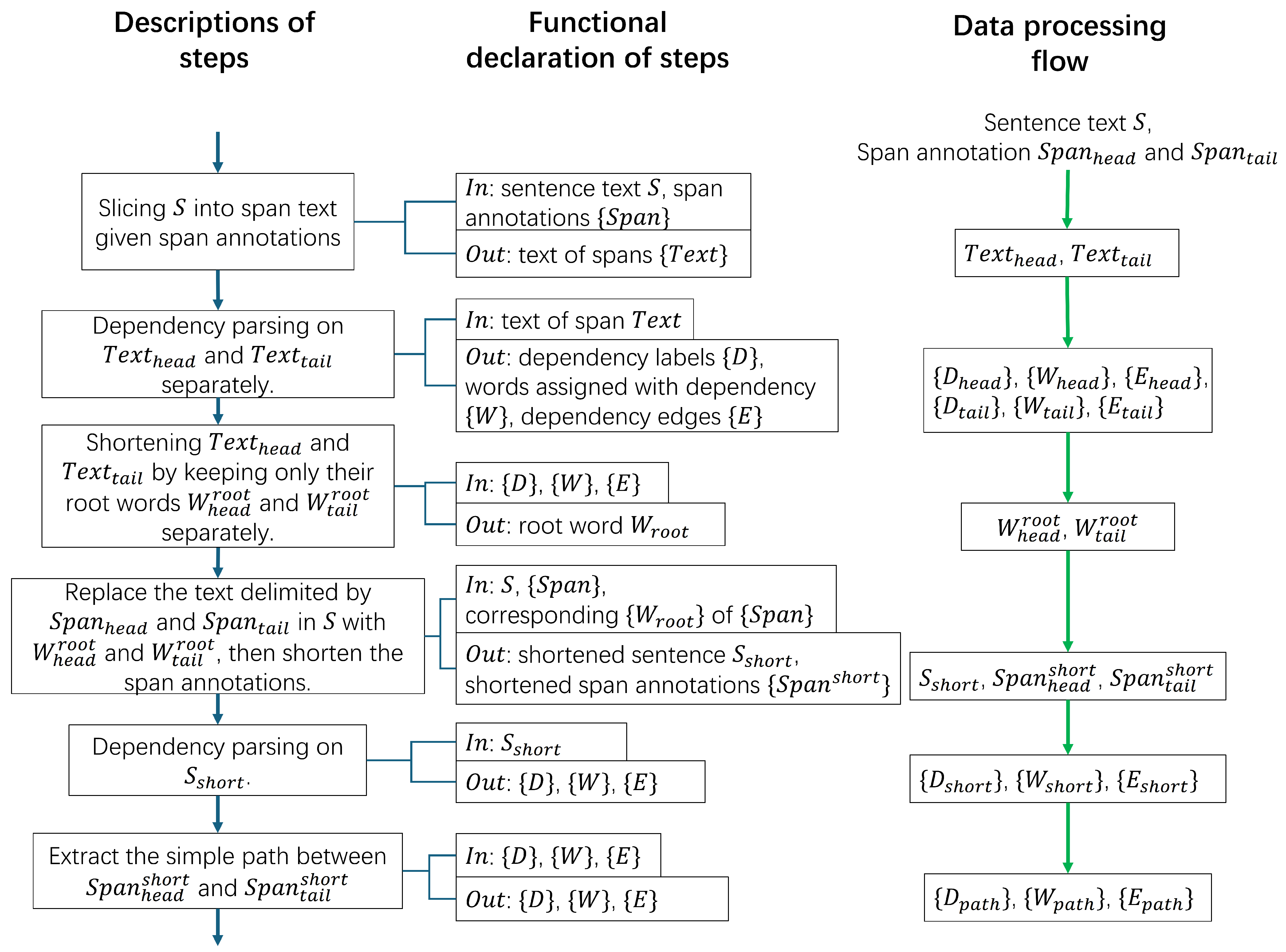
The pipeline from span shortening to path extraction is depicted in Figure 1. Given the sentence text S and the word index representations $Spa{n}_{head}$ and $Spa{n}_{tail}$, the text of head and tail entity ($Tex{t}_{head}$ and $Tex{t}_{tail}$) are obtained through text slicing. Then, text spans $Tex{t}_{head}$ and $Tex{t}_{tail}$ are shortened to two root words $W_{head}^{root}$ and $W_{tail}^{root}$, correspondingly, based on dependency parsing. Next, the original text in S of the entity pair are replaced with the two root words, correspondingly, which generates the shortened text $S_{short}$ and new word index representation $Spa{n}_{head}^{short}$ and $Spa{n}_{tail}^{short}$. Finally, $S_{short}$, $Spa{n}_{head}^{short}$, and $Spa{n}_{tail}^{short}$ are parsed again for extracting the simple path between the entity pair, generating words $\left\{w_{path}\right\}$, dependency labels $\left\{d_{path}\right\}$, and dependency edges $\left\{E_{path}\right\}$. Represented by index pairs, edges in $\left\{e_{path}\right\}$ are listed starting from the head entity and ending with the tail entity.

For revealing the contributions of collocation-level patterns, a path clustering scheme was designed to group the words along the path together into collocations, which incorporated the idea of span-based methods and was rarely discussed in the past efforts based on dependency graphs. The design scheme was inspired by the categorization of open class words and close class words in universal dependency scheme (https://universaldependencies.org/u/pos/index.html [accessed on 30 May 2025]), in which “open class words” referred to words that readily accepted new member words and otherwise “close class words”. Dependency labels in the designed clustering scheme are divided into three main groups, namely, the open group, the end group, and the special group only for dependency root, as in

Table 3. Groups of dependency labels for the design clustering scheme.

Groups	Dependency Labels
Open	[“acl”, “advcl”, “relcl”, “dobj”, “pobj”, “nsubj”, “nsubjpass”, “csubj”, “ccomp”, “pcomp”, “xcomp”]
Close	[“prep”, “agent”]
Special	[“ROOT”]

. Within an input dependency path, a word w with a dependency label in the open group is the start of new word collocation, as well as the end of the previous word collocation exclusively (i.e., not including w itself). Words with dependency labels the close group only marked the end of the current word collocation inclusively (i.e., including the word itself). A word collocation can only contain w if the previous word collocation does not exist or there are no words after a word with open dependency. The completed table of dependency labels for the path clustering scheme is provided in Appendix A (

Table A1. List of dependency labels used by the Spacy dependency parser, where descriptions under “description” categories are those modified for label verbalization and others under “original description” are provided along with Spacy transformer-based pipeline 3.2.0 release.

Label	Description	Original Description
acomp	complement adjectival	adjectival complement
ccomp	complement clausal	clausal complement
xcomp	complement clausal open	open clausal complement
pcomp	complement preposition	complement of preposition
attr	complement verb copular	attribute
agent	complement verb passive	agent
compound	compound	compound
conj	conjunct	conjunct
cc	conjunction coordinating	coordinating conjunction
preconj	conjunction pre correlative	pre-correlative conjunction
mark	conjunction	subordinating marker
dep	dependent	unclassified dependent
det	determiner	determiner
predet	determiner pre	pre-determiner
intj	interjection	interjection
amod	modifier adjectival	adjectival modifier
advmod	modifier adverbial	adverbial modifier
npadvmod	modifier adverbial	noun phrase as adverbial modifier
advcl	modifier adverbial	adverbial clause modifier
appos	modifier appositional	appositional modifier
acl	modifier clausal noun	clausal modifier of noun (adjectival clause)
meta	modifier meta	meta modifier
neg	modifier negation	negation modifier
nmod	modifier nominal	modifier of nominal
nummod	modifier numeric	numeric modifier
poss	modifier possession	possession modifier
case	modifier possessive	case marking
prep	modifier prepositional	prepositional modifier
quantmod	modifier quantifier	modifier of quantifier
relcl	modifier relative clause	relative clause modifier
dobj	object direct	direct object
dative	object indirect	dative
oprd	object predicate	object predicate
pobj	object preposition	object of preposition
parataxis	modifier parenthetical	parataxis
prt	preposition	particle
punct	punctuation	punctuation
ROOT	root	root
csubj	subject clausal	clausal subject
nsubj	subject nominal	nominal subject
csubjpass	subject passive clausal	clausal subject (passive)
nsubjpass	subject passive nominal	nominal subject (passive)
expl	there	expletive
aux	verb auxiliary	auxiliary
auxpass	verb auxiliary passive	auxiliary (passive)

).

Given the dependency groups, each edge in $\left\{e_{path}\right\}$ is traversed to determine the starts and ends of collocations, represented as index pair $(n_{start},n_{end})$. When $n_{start}$ corresponds to a local root (whose parent word is not within the path), only $n_{start}$ should be clustered to an existing word collocation if $n_{end}$ is the right/left end of the path. When $n_{end}$ belongs to the open group, $n_{start}$ should be clustered as the start of a new word collocation. Only $n_{end}$ should be clustered to an existing word collocation if $n_{start}$ has already been processed. If no special cases, $n_{start}$ and $n_{end}$ should be both clustered to an existing word collocation. The final output of path clustering can be represented as $\left\{C\right\}$, where C means collocation.

3.4. GAT for Relation Classification

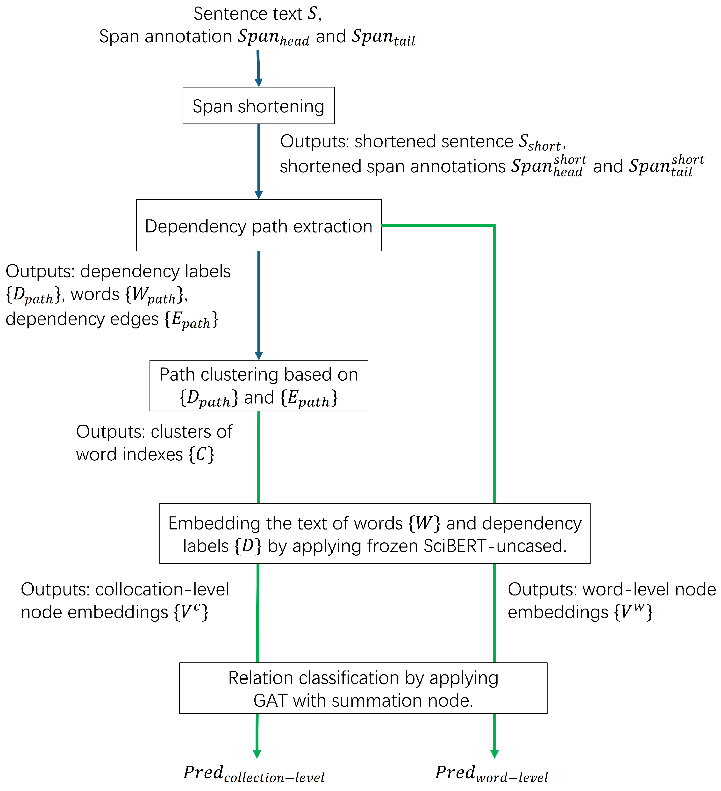
After extracting and clustering dependency paths, a GAT was applied for all experiments performing relation classification on extracted dependency paths. A brief overview of the proposed method is depicted in Figure 2. Compared to one of its popular competitors GCNs, GATs could process graphs with variant number of nodes and, thus, further consideration of padding was not needed. Meanwhile, the attention mechanism of the GAT could highlight the importance of each input node from the view of classifier after training and, thus, had suitable explainability. All GATs experimented on were trained on the training set of SciERC and then tested on the test set. The GAT implementation from pyGAT) was adopted and modified for performing relation classification. Following the graph-specific design of GNNs described in [16], the major input graph designs involved adding an extra node for summation, which was different from other nodes for words. In this design, the input nodes were linked directly to the added summation node. This input graph design adopting one summation node was adopted for two main reasons. First, this input graph design could reveal how much the word-level patterns within dependency paths could be used by GNN models for scientific relation classification. Simply linking the input nodes to the summation nodes means difficulty in explicitly utilizing the absolute positional information of words but easiness in reflecting the contribution of each input node’s content and, thus, it helped investigate word-level patterns and collocation-level patterns. Second, the adopted GAT architecture was the simplest case implementing graph pooling since it always tried to pool all the input nodes into one.

The modified GAT architecture was visualized in Figure 3. First, for an input sequence with N words, the embeddings of each word $w_i$ ($i\in 0,1,2,3,\dots ,n$) in the input sequence and its corresponding dependency label $d_i$ are concatenated as in Equations (2) and (3). Equation (2) is for investigating word-level semantic invariance, in which $V_i^w$ denotes the i-th word-level node embedding, $Emb(\dots )$ means embedding the input text, and $Concat(\dots )$ refers to the operation of concatenating multiple input embeddings; Equation (3) is for collocation-level invariance, in which $V_j^c$ denotes the j-th collocation-level embedding (“c” here is short for “collocation”), ${\sum }_{i\in c_j}Em{b}_{ctxt}\left(w_{i,j}\right)$ means summing the contextualized embeddings of words within word collocation $c_j$ (“ctxt” is short for “contextualized”), and ${\sum }_{i\in c_j}Em{b}_{static}\left(d_{i,j}\right)$ means summing the static embeddings of dependency labels within word collocation $c_j$. All embeddings were generated by applying frozen (i.e., non-trainable) SciBERT-uncased, the embedding size of which is 768 ($Siz{e}_{lm}=768$). Therefore, the size of node embedding is 1536 (i.e., $Siz{e}_{in}=1536$) after the concatenation. Second, the non-trainable embedding of the summation node $V_a$ (“a” stands for “aggregated”) is appended to the end of the node embeddings $[V_i^{in},\dots ,V_N^{in}$ to form $Em{b}_{in}$, as in Equation (4), where $V_{i}n$ is either $V^w$ or $V^c$. The embedding of summation node had the same size as that of an input node but was initialized with zeros since it had no corresponding semantic content and dependency information.

$Em{b}_{in}$ is processed using two GAT layers in order, which are $GA{T}_{hidden}$ (from $Siz{e}_{in}$ to $Siz{e}_{hidden}$) and $GA{T}_{out}$ (from $Siz{e}_{hidden}$ to $Numbe{r}_{class}$), as in Equation (5). For relation classification, the output embedding of the summation node was applied with softmax to get the probability $Probabilit{y}_{proposed}$ for each class, as in Equation (6). Specifically, $[:,-1,:]$ means selecting only the last element because $V_a$ is always appended at the end. The left branch in in Figure 3 depicts a GAT layer with multiple attention heads, where $GA{T}_0^{head}$ denotes the first head (from $Siz{e}_{in}$ to $Siz{e}_{hidden}/Numbe{r}_{head}$). Different with the one-head scenario shown as the right branch, the results of each head are concatenated and applied with ELU activation function.

$$\begin{array}{c}\hfill V_i^w=Concat(Em{b}_{static}\left(d_i\right),Em{b}_{static}\left(w_i\right)),\\ \hfill \mathrm{where}{d}_i\in \left\{d_{path}\right\},w_i\in \left\{w_{path}\right\}\end{array}$$

(2)

$$\begin{array}{c}\hfill V_j^c=Concat(\sum _{i\in c_j}Em{b}_{static}\left(d_{i,j}\right),\sum _{i\in c_j}Em{b}_{ctxt}\left(w_{i,j}\right)),\\ \hfill \mathrm{where}{c}_j\in \left\{c\right\},d_{i,j}\in \left\{d_{path}\right\},w_{i,j}\in \left\{w_{path}\right\}\end{array}$$

(3)

$$Em{b}_{in}=[V_i^{in},\dots ,V_N^{in},V_a]$$

(4)

$$Logi{t}_{out}=GA{T}_{out}\left(GA{T}_{hidden}\left(Em{b}_{in}\right)\right)$$

(5)

$$Probabilit{y}_{proposed}=Softmax\left(Logi{t}_{out}[:,-1,:]\right)$$

(6)

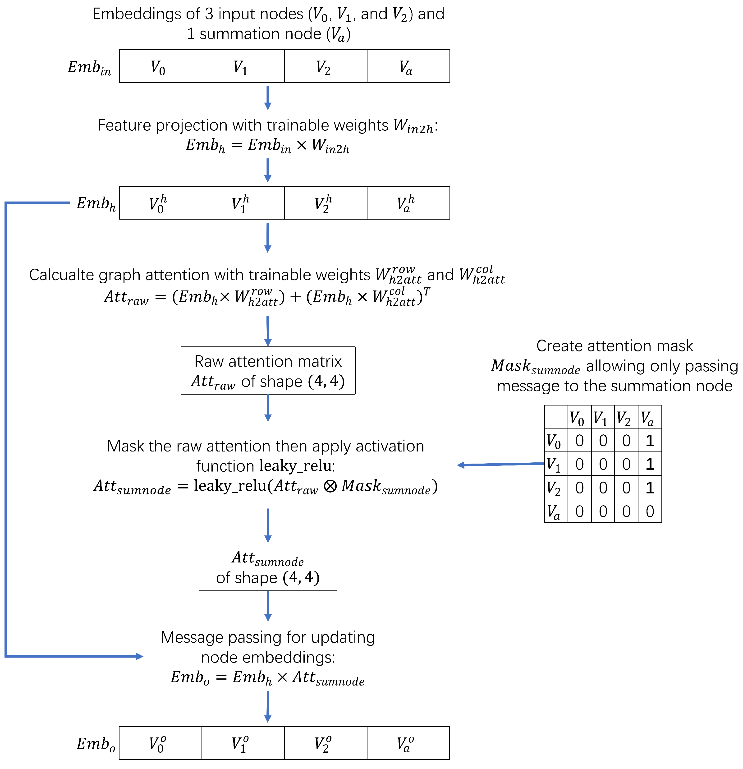
Within one GAT layer, the interactions between inputs and parameters are depicted in Figure 4, where only the three weight matrices $W_{in2h}$, $W_{h2att}^{row}$, and $W_{h2att}^{col}$ are trainable. $Em{b}_{in}$ here contains four nodes, the last of which is the summation node. First, input embeddings transformed by applying $W_{in2h}$ of shape $(Siz{e}_{in},Siz{e}_{hidden})$. Second, the raw attention scores $At{t}_{raw}$ of shape $(4,4)$ are calculated by applying $W_{h2att}^{row}$ and $W_{h2att}^{col}$ separately and then summing the rows and columns. Both $W_{h2att}^{row}$ and $W_{h2att}^{col}$ are of shape $(Siz{e}_{hidden},1)$. Third, the calculated $At{t}_{raw}$ is masked by $Mas{k}_{sumnode}$ via element-wise multiplication, denoted by ⊗. $Mas{k}_{sumnode}$ only allows summing information from $[V_0^h,V_1^h,V_2^h$ to $V_a^h$ by keeping only the edges from others to summation node. Finally, the updated embeddings $Em{b}_o$ is obtained by $Em{b}_h^{row}\times At{t}_{sumnode}$.

For revealing the contributions of word-level patterns, the embedding for each term in the SciBERT-uncased vocab file was collected from the last layer’s hidden state of SciBERT-uncased regardless of the context of input sentence to embed input words, which then generated static word embeddings. This static embedding method was adopted to ensure that only information within the extracted paths was used and, thus, ensured a focus on the word-level patterns for evaluating the potential of GNNs for scientific relation extraction. The embedding of a word was generated by first tokenizing it into SciBERT-uncased vocab terms and then performing a mean pooling on the static embeddings of these vocab terms (excluding the embeddings of [CLS] and [SEP]). To embed dependency labels, these labels were first verbalized following a bag-of-word idea, which used several words to express one label. The completed label verbalization scheme is provided in Appendix A (Table A1). Then, similar to embedding a single word previously, the static embeddings of the words describing a dependency label were collected and mean pooling was applied on. The embeddings of several words describing a label were averaged to simply ensure that similar labels had similar embeddings (e.g., in terms of cosine similarity). Since the dependency parsing results were generated following the idea of token classification, the embedding of a verbalized dependency label was concatenated to its corresponding word to form the embedding of a node in the input graph.

For revealing the contributions of collocation-level patterns, the embedding of each input node was a concatenation of two parts, which were the sum of contextualized vocab term embeddings of their corresponding words in the word collocation and the sum of dependency label embeddings of their corresponding words in the word collocation. The dependency label embedding of each word was obtained in the same way in the experiments for revealing word-level patterns. The contextualized embeddings of vocab terms for their corresponding words were first obtained in the context of the shortened sentences and then summed, which were generated after applying the span shortening described in Section 3.3. Similarly, the embedding of [CLS] or [SEP] token were not included in the final calculation of node embeddings. Instead of using static embedding, the contextualized embeddings were adopted for performance optimization, since the semantics of a word collocation depended more on the word order.

3.5. Configurations of Experiments

The configuration of hyperparameters is provided in

Table 4. Hyperparameters for training the GAT.

Hyperparameters	Values
Hidden size $Siz{e}_{hidden}$	200
Number of heads $Numbe{r}_{head}$	1
Dropout	0
Negative slope for leaky ReLU	0.01
Alpha for ELU	0.2
Learning rate	0.0005
Epochs for training	200

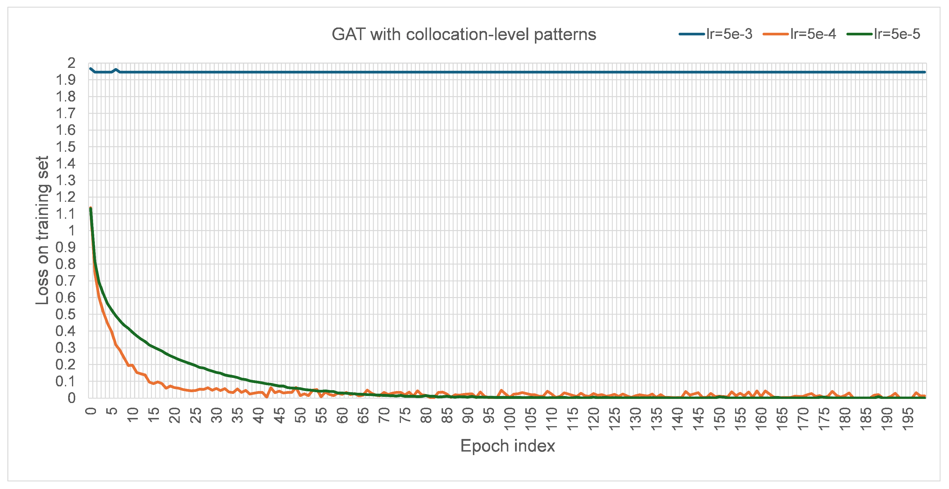
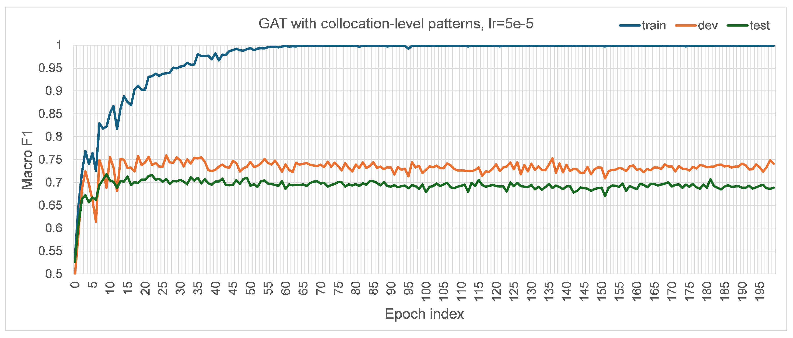
. The hidden size was set to 200 following [8,27] for convenient comparison. The number of heads was initially set to one. The dropout rate was set to zero to maintain all information currently. The negative slope of leaky ReLU was set to 0.01, following the default PyTorch 2.0.1 implementation; similarly, the alpha value for ELU was set to 0.2 following the default implementation. Every model was trained for 200 epochs to experiment with their ability to fit into the training set and generalization on the development set, based on which the models were considered if they were worth further training. The loss for training the designed GAT models was chosen to be cross-entropy loss. The learning rate was set to 0.0005 after some initial experiments trying {0.5, 0.05, 0.005, 0.00005}. When the learning rate was set to 0.5 and 0.05 with other hyperparameters unchanged, the losses were stuck at 1.9458. For 0.005, 0.0005, and 0.00005, their corresponding performance trends with the growth of training epochs in terms of macro F1 are visualized in Appendix A (Figure A2,Figure A3,Figure A4), correspondingly. Apparently, the best performance with the learning rate of 0.005 on the test set was lower than those with the learning rate of 0.0005 and 0.00005, so it was not used for experiments. For the learning rate of 0.00005, the best performance in macro F1 on the test set was 0.6544, which was slightly lower than the performance with the learning rate of 0.0005. Since using a small learning rate would usually slow the convergence during model training, the larger learning rate of 0.0005 was preferred and adopted. The default parameters of the Adam [41] optimizer implemented in PyTorch 2.0.1 and a random seed value of 42 were used to train the model.

To evaluate the effectiveness of different models in the classification of scientific relations, four classification criteria including accuracy, precision, recall rate, and macro F1 score were used, which had also been used in previous studies. The macro F1 score was considered the main criterion as it takes into account both precision and recall rate, which under the multi-classification settings was calculated as the average of the F1 score of each class. Provided a sequence of model prediction results and their corresponding ground-truth values, precision, recall rate, basic F1 score, and macro F1 score are expressed in (7)–(11), where $T_p$ is for the number of true positives (e.g., the samples both annotated and predicted as “USED-FOR”), $F_p$ for the number of false positives (e.g., the samples both annotated and predicted as not “USED-FOR”), $F_n$ for the number of false negatives (e.g., the samples annotated as “USED-FOR” but predicted as “USED-FOR”), and $n_{relation}$ is the enumeration of all natural numbers that are smaller than the number of relations.

$$Accuracy={\displaystyle \frac{N_{matched}}{N_{samples}}}$$

(7)

$$Precision={\displaystyle \frac{T_p}{T_p+F_p}}$$

(8)

$$Recall={\displaystyle \frac{T_p}{T_p+F_n}}$$

(9)

$$F1=2{\displaystyle \frac{P\times R}{P+R}}$$

(10)

$$F1=\sum _{i\in n_{relation}}{\displaystyle \frac{F{1}_i}{n_{relation}}}$$

(11)

The relation classification task on SciERC was formalized as two types: multi-classification and bi-classification. For multi-classification, the input samples covered all seven relation types, and a classification model was expected to choose the most suitable relation from the seven types for an input sample. This multi-classification design followed previous extraction studies on SciERC for convenient comparison. For bi-classification, input samples covered only two types indicating whether a sample was for a relation or not. Under this design, seven datasets were produced for each relation. This bi-classification formalization was designed to reveal the performance of the designed GAT for each relation type individually. To accommodate the two settings, the output size of the designed models was set to seven and two for multi-classification and bi-classification, respectively.

3.6. Comparative Methods

For demonstrating the ability and gaps of the experimented models, the benchmark model [21] applied one linear layer on SciBERT-uncased and then finetuned it for classifying all seven relations. The architecture followed by the benchmark method is depicted in Figure 5. Different from our classification design, the benchmark model feeds the embedding of [CLS] token to the linear classifier layer to obtain the for similar to [8]. However, using [CLS] embedding for classification raises the problem of distinguishing different entity pairs in the same input sentence. Hence, to mark the head and tail entities, text symbols were used by the benchmark model to prompt the model. For example, in the sample “One is « string similarity » based on [[ edit distance ]]”, the symbol pair “[[” and “]]” is used to prompt the span within the pair as head entity; the symbol pair “«” and “»” is used to prompt the span within the pair as tail entity. This prompt design requires the user to rerun the whole language model each time when processing a new entity pair in the same sentence. For classifying one entity pair, the prompted text is first tokenized into input sequences and then fed to SciBERT-uncased to obtain contextualized embedding of [CLS] token ($Em{b}_{\left[CLS\right]}$), as in Equation (12). In Equation (12), $Prompt(\dots )$ refers to the text function that mark entity pairs with the symbols; $[0,\dots ]$ is an indexing operation that return the first embedding of the input embedding sequence, which is normally the embedding of [CLS] token for SciBERT models. The $Logi{t}_{out}^{\prime }$ used for final classification is obtained by applying the linear classifier layer on the [CLS] embedding as in Equation (13), where $Laye{r}_{Linear}$ is the linear classifier layer and matrix $Weigh{t}_L$ of shape $(Siz{e}_{hidden},Numbe{r}_{class})$ and $bia{s}_L$ of shape $\left(Numbe{r}_{class}\right)$ are its parameters. Finally, $Logi{t}_{out}^{\prime }$ is applied with softmax to get the probabilities $Probabilit{y}_{benchmark}$ for each class, as in Equation (14).

$$Em{b}_{\left[CLS\right]}=SciBER{T}_{uncased}\left(Tokenizer\left(Prompt\left(Text\right)\right)\right)[0,\dots ]$$

(12)

$$Logi{t}_{out}^{\prime }=Laye{r}_{Linear}\left(Em{b}_{\left[CLS\right]}\right)=Em{b}_{\left[CLS\right]}\times Weigh{t}_L+bia{s}_L$$

(13)

$$Probabilit{y}_{benchmark}=Softmax\left(Logi{t}_{out}^{\prime }\right)$$

(14)

The benchmark model was chosen since its architecture was simple enough to reflect the effectiveness of utilizing dependency graph information. Moreover, it was the only up-to-date work focusing on comprehensively discussing SciBERT scientific relation classification across each SciERC relation to our best knowledge, while other studies also considered extracting the expected span pairs as in Section 3.2 task definition, which may add unnecessary complexity to reflect the effectiveness. The benchmark performance to compare for both of the task formalizations was obtained from [21]. The performance of the benchmark on all relations is only provided in accuracy and macro F1, which are 0.8614 and 0.7949, correspondingly. The performance of the benchmark on each relation is provided in

Table 5. Performance of relation classification on SciERC (P, R and F1 stands for precision, recall, and F1, correspondingly) for comparison. Evaluation results in bold indicates the best performance.

Relation	Method	A	P	R	F1
Used-for	Benchmark	-	0.9330	0.9137	0.9232
	MRC	-	0.8875	0.9024	0.8949
Conjunction	Benchmark	-	0.8797	0.9512	0.9141
	MRC	-	0.8069	0.9512	0.8731
Hyponym-of	Benchmark	-	0.9231	0.8955	0.9091
	MRC	-	0.8000	0.8293	0.8144
Evaluate-for	Benchmark	-	0.8229	0.8681	0.8449
	MRC	-	0.8444	0.8352	0.8398
Compare	Benchmark	-	0.7273	0.8421	0.7805
	MRC	-	0.8387	0.6842	0.7536
Part-of	Benchmark	-	0.6604	0.5556	0.6034
	MRC	-	0.6552	0.6032	0.6281
Feature-of	Benchmark	-	0.5902	0.6102	0.6000
	MRC	-	0.7368	0.4746	0.5773

. Provided the absence of bi-classification in the original work and our limited computation resources, the benchmark performance under multi-classification was also used in comparison with the designed graph-based models for subsequent analysis. The benchmark model achieved a performance suitable for application but required significantly more computation resources during training than the proposed method. A comparison of the finetuned/trained parameters between the benchmark model and the proposed method is shown in

Table 6. Parameter levels of proposed method compared to the benchmark model. “M” stands for million.

Method	Parameter Level
Benchmark	About 110 M
GAT-sumnode one-head	About 0.3 M
GAT-sumnode two-head	About 0.6 M

, where “one-head” means using one attention head for GATs and “two-head” means using two.

In addition, a method named MRC was compared, which is short for multiple-relation-at-a-time classification. MRC modifies the self-attention mechanism of transformer architecture so that the representations of the relative positions of entities are considered [21]. In other words, additional parameters are added to the SciBERT model while the pretrained parameters of SciBERT-uncased can still be directly loaded. Apart from this change, MRC adopts the same data and architecture as the benchmark model, which means it shares the Equations (13) and (14). Also using SciBERT-uncased, the performance of MRC on all relations is only provided in accuracy and macro F1, which are 0.8433 and 0.7744, correspondingly. The performance of MRC on each relation is provided in Table 5. Similarly, the benchmark performance under multi-classification was also used in comparison with the proposed method.

4. Results

The results of performed experiments under multi-classification configuration are shown in

Table 7. Best observed performance of designed GAT models based on macro F1 on SciERC test set under multi-classification configuration (A, P, R, and macro F1 stands for accuracy, precision, recall, and F1, correspondingly). Evaluation results in bold indicate the best performance; underlined evaluation results for the proposed method surpasses those of MRC while not being the best.

Configuration	A	P	R	F1
Summation (word-level)	0.7843	0.6901	0.6590	0.6701
Summation (word-level) + 2 heads	0.7843	0.7014	0.6510	0.6700
Summation (collocation-level)	0.8521	0.7945	0.7507	0.7682
Benchmark	0.8614	-	-	0.7949
MRC	0.8433	-	-	0.7744

. Both the accuracy and macro F1 score of the designed GAT model focusing on word-level patterns are lower than those of the benchmark model by about 0.1, while adding extra attention heads for the designed GAT architecture did not guarantee a better performance in terms of macro F1. In comparison, both the accuracy and macro F1 score of the designed GAT model focusing on collocation-level patterns are closer to those of the benchmark model, with the gap being only 0.01 and 0.03, correspondingly. However, collocation-level GAT slightly outperformed MRC in terms of accuracy and reached a comparative F1 score with MRC. The designed GATs with collocation-level patterns outperformed those with word-level patterns, demonstrating the stronger contribution of collocation-level patterns for scientific relation extraction on SciERC.

Under the bi-classification setting, the best performance on the SciERC test set of each relation is shown in

Table 8. Best observed performance of designed GAT models based on macro F1 on SciERC test set under bi-classification configuration, with word-level node content (A, P, R, and F1 stands for accuracy, precision, recall, and macro F1, correspondingly). Evaluation results in bold indicate the best performance; underlined evaluation results for the proposed method surpasses those of MRC while not being the best.

Relation	Method	A	P	R	F1
Used-for	Proposed	0.8470	0.8477	0.8430	0.8447
	Benchmark	-	0.9330	0.9137	0.9232
	MRC	-	0.8875	0.9024	0.8949
Conjunction	Proposed	0.9671	0.9231	0.9290	0.9260
	Benchmark	-	0.8797	0.9512	0.9141
	MRC	-	0.8069	0.9512	0.8731
Hyponym-of	Proposed	0.9702	0.9034	0.8526	0.8760
	Benchmark	-	0.9231	0.8955	0.9091
	MRC	-	0.8000	0.8293	0.8144
Evaluate-for	Proposed	0.9486	0.8652	0.8139	0.8371
	Benchmark	-	0.8229	0.8681	0.8449
	MRC	-	0.8444	0.8352	0.8398
Compare	Proposed	0.9753	0.8581	0.7852	0.8171
	Benchmark	-	0.7273	0.8421	0.7805
	MRC	-	0.8387	0.6842	0.7536
Part-of	Proposed	0.9291	0.6978	0.6592	0.6758
	Benchmark	-	0.6604	0.5556	0.6034
	MRC	-	0.6552	0.6032	0.6281
Feature-of	Proposed	0.9517	0.7990	0.7364	0.7634
	Benchmark	-	0.5902	0.6102	0.6000
	MRC	-	0.7368	0.4746	0.5773

and

Table 9. Best observed performance of designed GAT models based on macro F1 on SciERC test set under bi-classification configuration, with collocation-level node content (A, P, R, and F1 stands for accuracy, precision, recall, and macro F1, correspondingly). Evaluation results in bold indicate the best performance; underlined evaluation results for the proposed method surpasses those of MRC while not being the best.

Relation	Method	A	P	R	F1
Used-for	Proposed	0.9004	0.8993	0.8998	0.8995
	Benchmark	-	0.9330	0.9137	0.9232
	MRC	-	0.8875	0.9024	0.8949
Conjunction	Proposed	0.9640	0.9247	0.9098	0.9171
	Benchmark	-	0.8797	0.9512	0.9141
	MRC	-	0.8069	0.9512	0.8731
Hyponym-of	Proposed	0.9691	0.8730	0.8936	0.8830
	Benchmark	-	0.9231	0.8955	0.9091
	MRC	-	0.8000	0.8293	0.8144
Evaluate-for	Proposed	0.9681	0.9300	0.8740	0.8995
	Benchmark	-	0.8229	0.8681	0.8449
	MRC	-	0.8444	0.8352	0.8398
Compare	Proposed	0.9876	0.9178	0.9178	0.9178
	Benchmark	-	0.7273	0.8421	0.7805
	MRC	-	0.8387	0.6842	0.7536
Part-of	Proposed	0.9527	0.8517	0.7014	0.7528
	Benchmark	-	0.6604	0.5556	0.6034
	MRC	-	0.6552	0.6032	0.6281
Feature-of	Proposed	0.9589	0.8503	0.7482	0.7891
	Benchmark	-	0.5902	0.6102	0.6000
	MRC	-	0.7368	0.4746	0.5773

. Compared to the benchmark and MRC, obvious improvement in macro F1 was observed on the test set for three relation types when focusing on word-level patterns: Feature-Of, Part-Of, and Compare. The bi-classification performance on Conjunction was the best and even higher than that of the benchmark, while comparable performance was observed for relation Evaluate-for. When focusing on collocation-level patterns, general performance was observed on the test set except for three relation types Used-for, Conjunction, and Hyponym-of.

The experiments under the bi-classification setting also revealed how distinctive one relation type was to others from the perspective constructed based on the dependency graph, since the designed input graphs of GAT directly measured the importance of each input node to the final decision. Among others, the samples with Compare, Part-Of, and Feature-Of could not be distinguished from others as successfully as others when focusing on word-level patterns, based on the recall rate (less than 0.8). When focusing on collocation-level patterns, the ability of designed GAT models to distinguish relation types was generally improved except for Hyponym-of and Conjunction. The minor improvement and even slight reduction of the performance on the two relation types indicated that the contribution of word-level patterns was already strong in distinguishing samples of these relation types from others. To sum up, the best performance of designed model was promising. The performance of GAT models with collocation-level patterns trained under bi-classification configuration was already more suitable for extracting five relations from scientific text than the benchmark, which were Used-for, Conjunction, Hyponym-of, Evaluate-for, and Compare.

5. Discussion

The overall performance improvement from focusing on word-level patterns to collocation-level patterns in dependency graphs demonstrated that more semantic invariance were learned by the designed models, provided the challenge of “New” samples mentioned in Section 3.1. However, to outperform the benchmark mainly based on finetuning, more semantic invariance should be learned by the models, which can be directly reflected in the input embeddings. Shallow models such as the designed GAT architecture in this work relied heavily on the input embeddings generated by large pretrained language models (PLM) such as BERT. Although PLMs can be finetuned to fit the distribution of domain-specific language such as SciBERT, the cost of finetuning is expensive, especially when the domain-specific language is frequently expanded with newly emerged concepts and links. Therefore, it is necessary to have lightweight solutions or workarounds that are flexible and robust for scientific relation extraction.

5.1. Integrating and Extending Input Graphs

To achieve the expected effect of scientific relation extraction, a direct solution for learning more semantic invariance is about integrating external semantic knowledge bases such as WordNet [42] to improve the quality of input embeddings [43]. With the continuous expansion of scientific language, no matter how large the training data set is, there may still be unseen trigger words in the test set. Provided the high dimensionality of the embedding of natural language, classification models classifying unseen samples in its training set are referred to as extrapolation while classifying seen samples as interpolation [44]. To control the extrapolation behavior for scientific relation extraction, it is possible to let the model recognize the rare and even unseen semantic content as similar to the seen content and, thus, enhance learned semantic invariance. This conversion from unseen to familiar can be helped by using annotated data such as synonyms annotated in WordNet. Integrating annotated domain-specific expressions from other scientific knowledge graphs or bases can not only help in the basic conversion but also enable flexible conversion when the input text is from multiple domains. However, integrating edges and nodes from external knowledge bases can raise further problems of how to design the input graphs for fusing the external information.

Next, to enhance semantic invariance that can be learned by graph-based models, careful path extension can be considered. As mentioned in some previous graph-based studies in Section 2.2, in-path information may not be enough for models to generate correct decisions, leading to the development of path extension. However, there are still problems with finding where to stop extending a path. A typical example identified from the training set of SciERC is shown in Figure 6, and it cannot be resolved by the existing path-extending methods except by keeping the whole graph. For the example in Figure 6, this type of off-path information can be included if it considers the path from the root word of the original sentence to the span that is closest to it, but more irrelevant information may, thus, be included. For further processing the irrelevant information in the extracted dependency paths, path integration can be considered, which focuses on processing the dependencies among the extracted paths. For example, different extracted paths could be integrated based on shared relation label space [45] and shared word collocation. However, both path integration and path extension require upgraded input graph design to aggregate the expected information for the final classification.

5.2. Next GNN Could Be Beyond GNN

Towards improved scientific relation extraction, the next GNN architecture can be transitioned to transformer-based architecture. Although there is evidence that GNN performs well in classifying scientific text on citation network datasets like Cora, when the analysis is narrowed down to words or word collocations from documents, there is still a gap in the GNN’s ability to surpass the finetuned SciBERT, as demonstrated in experiments. As shown in the experimental results of using two attention heads, it can be expected that increasing the number of attention heads will bring marginal or even negative benefit to the final performance, indicating the limitation of the GNN architecture. The potential of increasing attention head may be further utilized if they are trained to separately react to specific patterns, but this requires more specific input graph design (i.e., inductive bias), presenting challenges for enhancing performance.

For exceeding the finetuned SciBERT, a promising way can be transitioning the current GNN architecture such as GAT-based and GCN-based to more transformer-based architecture, since SciBERT is developed from the encoder part of the original transformer. With the similarity to GATs in applying attention architecture, the transformer can be understood as a specific type of GNN when tokens or token sequences are treated as nodes [46]. In particular, the summation node design also shares a high similarity with the autoregressive behavior of a typical transformer decoder, because at each time step, choosing the next token to generate requires weighting and then summarizing the information from all input tokens. Witnessing the success and trend of training and applying large transformer-based models [47], transformer-based GNN architecture with specific input and behavior designs in both the encoder and decoder can further enhance the performance of scientific relation extraction with the previously discussed methods.

5.3. Extendibility and Limitations

The proposed method can be extended to tasks that can be reduced to classifying entity pairs under specified textual context. Because we have not integrated domain-specific external knowledge bases to enhance final performance, the proposed method is applicable to generic relation extraction, normally regardless of text topics; to improve performance on specific tasks, the knowledge bases can then be adopted to enhance the context. However, for relation extraction tasks that assign relation classes mostly based on occurrences of certain entity pairs instead of overall context (usually reflected in their annotation scheme), using dependency parsing may be redundant. Although the proposed method is extendable, it has certain limitations. First, due to the task definition, the proposed method is specifically designed for binary relation extraction. Extending the method to n-ary relation extraction requires further processing of extracted paths so that all entities can be traversed. Second, the method is limited by the max context length (512 tokens) of the dependency parsing model. Hence, for text containing terminology with long names (e.g., the full names of certain chemical substances) and document-level relation extraction, the input context should be preprocessed to avoid exceeding max length. Thirdly, as the core component of the proposed pipeline, the performance of dependency parsing and post-processing quality of the parsing results also limit the performance of relation extraction. The dependency parser can easily mistake the dependency between words when there is an in-context listing marked with indexes. Because common dependency parsers are not trained to allow guidance, careful post-processing is needed.

6. Conclusions

Building upon the devised GAT models, this work introduces an innovative GNN-based pipeline that leverages dependency graphs for scientific relation extraction. The proposed lightweight architecture, particularly in bi-classification scenarios, has already demonstrated its effectiveness, notably in classifying five key relations: Used-for, Conjunction, Hyponym-of, Evaluate-for, and Compare. Attributed to a focus on collocation-level patterns, the improved performance showcases a more profound semantic invariance compared to that on word-level patterns.

To achieve a more flexible and robust knowledge integration through the construction of scientific knowledge graphs, it is imperative to further enhance the learned semantic invariance. This necessitates a deeper exploration of input graph designs, serving as the basis for solutions such as integrating external semantic knowledge bases and extending and integrating dependency paths. Furthermore, a promising approach involves transitioning the current GNN architecture towards a transformer-based model, supporting improved input graph design and enhancing relation extraction.