Energy Scheduling of PV–ES Inverters Based on Particle Swarm Optimization Using a Non-Linear Penalty Function

Abstract

The photovoltaic (PV) energy storage (ES) inverter is an effective way to solve the problems of energy shortage and environment pollution. However, when considering the constraints such as economic benefits and power supply reliability, the energy optimization and dispatching of this PV–ES system poses great challenges. This paper proposes an optimization method based on the combination of the particle swarm algorithm and non-linear penalty function to dispatch the energy of household PV–ES inverter. Based on the established optimization model of the PV–ES inverter system, compared with the static penalty function, the penalty factor can be automatically adjusted according to the range beyond the constraint by using the proposed non-linear penalty function. Furthermore, the particle swarm algorithm is used as the optimization engine, and the energy scheduling scheme is obtained by the combination of the particle swarm algorithm and the proposed non-linear penalty function. Finally, the simulation and hardware-in-the-loop results verify the correctness of the proposed algorithm, compared with the static penalty function, the user electricity expenses can be effectively reduced, and economic requirements can be met.

1. Introduction

In recent years, people’s enthusiasm for the development of renewable energy has gradually heightened due to the increasingly tight reserves of fossil energy [1,2]. Solar energy has become one of the most popular renewable energy sources due to its safety and cleanliness [3,4]. PV (PV) energy storage inverters are important products for the development of solar energy [5,6]. For this type of inverter, when the energy of each part of the system is properly dispatched, it can bring good social and environmental benefits [7,8]. For instance, after obtaining the PV power generation and load power consumption of the inverter system, the internal energy of the system can be scheduled and managed to avoid energy waste and reduce the daily electricity expenditure of users. However, how to maximize economic benefits by reasonably utilizing PV modules, energy storage units and power grids to supply power to household loads, is a multiple constraints optimization problem worthy of study.

To optimize energy management while maximizing economic benefits, there are mainly two types of methods: the conventional energy management method [9] and the advanced optimization-based algorithms [10,11,12,13,14,15]. For the conventional energy management method [9], when the power generation of PV modules exceeds the electricity consumption of the household loads, all the electricity of the loads is borne by the PV modules. When the charged state and all other constraint conditions of the energy storage battery module meet the specified requirements at this time, the excess electricity in the PV modules can continue to charge the battery. When there is still surplus electricity generated by the PV modules, and the battery reaches maximum state of charge, all the excess electricity will be fed back to the power grid. Conversely, when the electricity generated by the PV modules is insufficient to meet the demand of the household loads, and the battery module has not reached the minimum state of charge at this time and meets all relevant constraints, the electricity consumption of the household loads is jointly borne by the PV modules and the battery. When the battery is discharged to the minimum state of charge but still cannot meet the power demand of the loads, then the user has to purchase the remaining required electricity from the power grid. However, the downsides of the inherent uncertainty of solar energy and residential load due to their volatile nature are not considered in the above process, which is a challenge for the conventional energy management method. To mitigate the impact of the uncertainty, advanced optimization-based algorithms are effectively approached [10,11,12,13,14,15]. A stochastic dual dynamic programming (DP) algorithm was developed in [10] to minimize the electricity purchasing cost of residential buildings with PV-storage systems and electric vehicles under load and PV generation uncertainty. In [11], a stochastic model predictive control (SMPC)-based framework for the real-time operation of residential-scale DC-coupled PV-storage systems is proposed. Being a short horizon optimization problem, the SMPC has a low computation complexity and can easily incorporate the updated values of the uncertainty forecasts. Ye et al. [12] proposes a novel real-time autonomous energy management strategy for a residential multi-energy system using a model-free deep reinforcement learning (DRL)-based approach, combining state of-the-art deep deterministic policy gradient (DDPG) method with an innovative prioritized experience replay strategy. In [13], when there are modeling errors due to control delay, disturbances, and/or testing using a high-fidelity model (HFM) of the vehicle, the DRL-trained policy performs better when the modeling errors are large, while having similar performances as SMPC when the modeling errors are small. However, in these previous methods, more advanced optimization-based algorithms were developed to obtain better performance and handle more complex calculations. In references [14,15] particle swarm optimization (PSO) algorithms were utilized to solve optimization models with economic and environmental objectives. However, for optimization models involving multiple constraints, single optimization algorithms often struggle to identify high-quality solutions. The method of penalty function is an effective way in constraint processing.

For penalty functions, there have been developed multiple improved methods [16,17,18,19]. In [16], a metric penalty function is proposed to completely ignore the valid information of infeasible solutions in population evolution. When all the individuals in the initial species group are unsolvable, the penalty coefficients of all the individuals in the species group are zero, and the initial species group needs to be reformed at this time. However, the method of metric penalty function is not suitable for covenant problems with a low feasible ratio. In [17], the value of penalty coefficient in the process of species group evolution is designed as a constant. However, during the process of population evolution, many unreasonable situations of penalty coefficient values often occur and, thus, the effect is not positive. Reference [18] proposes a dynamic penalty function method, in which the penalty coefficient changes with the variation in evolutionary generations. Compared with the static penalty function and the metric penalty function, the dynamic penalty function can better adapt to the constraint problem and is superior in performance. The drawback is that repeated experiments are needed to find the ideal initial penalty system. An adaptive penalty function is proposed in [19], the penalty coefficient is, thus, adjusted by using the feasible ratio in the previous species group (the proportion of feasible solutions in the species group), thereby controlling the intensity of the penalty. However, the adaptive function is relatively complex.

In this paper, a non-linear penalty function method is proposed for the PV-storage inverter system, with the following key advantages:

(1)

With the non-linear penalty function method, the penalty factor in the iterative process is continuously updated to make the search result closer to the optimal value.

(2)

The particle swarm optimization algorithm serves as the search engine, combining the non-linear penalty function method to optimize the charge/discharge scheduling of energy storage batteries and the power transactions between users and the grid, thereby achieving enhanced user economic benefits.

The rest of this article is organized as follows: Section 2 presents the optimization model of the PV-storage inverter system; in Section 3, the non-linear penalty function method is discussed in detail; Section 4 presents the detailed process of the particle swarm optimization algorithm based on the non-linear penalty function; Section 5 and Section 6 provide simulation results and results analysis to verify the effectiveness of the proposed solution; and Section 7 concludes this article.

2. System Model

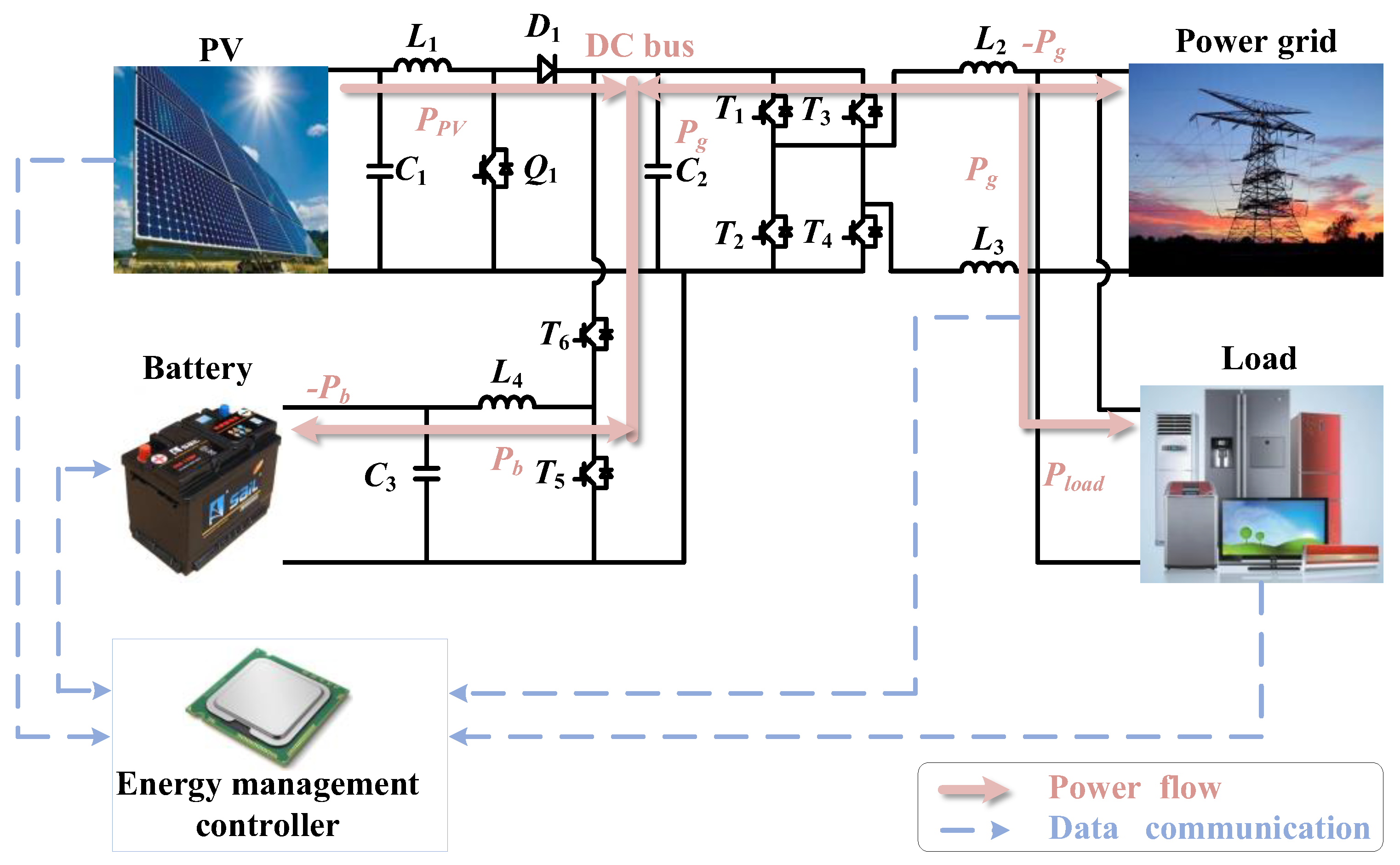
2.1. System Structure

The system structure of the PV-storage inverter system studied in this paper is shown in Figure 1. The PV section converts solar energy directly into electricity through the PV effect. The front-stage boost DC converter module (BDC), due to the simple structure, high efficiency, and strong compatibility with the MPPT algorithm, performs maximum power point tracking (MPPT) for the PV panels to maximize PV power generation revenue, which can significantly improve the efficiency of energy conversion. L₁, D₁ and Q₁ are the boost inductor, diode and switch of the BDC, respectively. The buck-boost converter module functions as the bridge between the DC bus and the battery module, facilitating energy management control through its bidirectional energy flow capability. This converter supports a wide voltage adaptability range, operates with high efficiency, and offers precise control characteristics. Consequently, the battery module can both receive energy from other components for charging and discharging to supply power to the load via the inverter module (SPTI). L₄, T₅ and T₆ are inductor and switches of the buck-boost converter module, respectively. The local load in the diagram represents the household user end connected to the output of the PV-storage inverter. Due to the low cost, compatibility with home power grids, and simple control, the single-phase inverter functions as the PV-storage inverter and connects the DC bus to the grid. This setup can either supply power to the load user end or purchase power from the inverter system. The full bridge of inverter consists of switches T₁–T₄, with L₂ and L₃ serving as output filter inductors. Optimization is performed using MATLAB R2023b on a PC with an Intel Core i5-4600U 1 GHz CPU, 4 GB of RAM, and 64-bit Windows 10 operating system. This inverter system operates in the three following power supply modes: (1) inverter-only power supply mode, as the power flows along with blue line; (2) grid-only power supply mode, as the power flows along with orange line; and (3) combined inverter-grid power supply mode, the power flows along the gray line.

The PV power generation in the system exhibits uncertainty, primarily associated with external factors such as irradiance, while the load power consumption also demonstrates randomness. Therefore, intelligent algorithms such as neural networks are generally employed to predict the power of PV generation and load consumption prior to energy optimization.

2.2. Mathematical Model

Under time-of-use electricity pricing, PV power electricity generation and load electricity consumption are obtained, the charging and discharging of the storage battery and the power trading situation between the system and the power grid is reasonably dispatched to make users meet their power requirements while maximizing user benefits and saving energy. In fact, it is a typical single-objective multi-constraint optimization problem; therefore, establishing the mathematical model is the basis of this optimization problem [10]. While the optimization problem includes two parts: objective function and constraint conditions, the purpose of the research is to find the minimum value of the objective function.

2.2.1. Objective Function

The electrical energy sources of the entire system are PV modules, battery storage, and the grid. Since PV power output cannot be artificially controlled, rational dispatch of power output from the grid and battery storage is sufficient to ensure optimal resource utilization. Due to the costs associated with planning, installation, and maintenance, such as expenditures on PV panels and battery storage, which constitute sunk costs, these factors are not considered in this model. Therefore, the final objective function can be expressed as:

$$J_c={\displaystyle \sum _{t=1}^T(E_{buy}}(t)\cdot f_{buy}(t)-E_{sell}(t)\cdot f_{sell}(t))$$

(1)

where J_c is the total cost, T is the optimization time, which is 24 h in this article; E_buy represents the amount of electricity purchased from the power grid at the tth h; f_buy represents the price of electricity purchased in the tth h; E_sell represents the amount of electricity sold to the power grid in the tth h; and f_sell represents the price of electricity sold in the tth h.

2.2.2. Constraint Condition

The constraint conditions for energy scheduling in PV storage inverter systems include system power balance constraint, grid output power constraints, and battery constraints.

The power balance constraint can be expressed as follows:

$$P_g(t)+P_b(t)+P_{pv}(t)=P_{load}(t)$$

(2)

where P_pv represents the power of the PV generation unit. P_b denotes the power provided by the energy storage unit, where a positive value indicates battery discharging and a negative value indicates charging. P_g is the power supplied by the grid, with a positive value representing electricity purchase from the grid and a negative value indicating electricity sale to the grid. P_load represents the load power.

The grid power transaction constraint can be expressed as

$$-P_{g\_\max }\le P_g(t)\le P_{g\_\max }$$

(3)

where P_{g_max} is the maximum power supplied by the grid.

The battery constraints can be expressed as follows:

$$-P_{bc\_\max }\le P_b(t)\le P_{bd\_\max }$$

(4)

$$Do{D}_{\min }\le DoD(t)\le Do{D}_{\max }$$

(5)

$$So{C}_{\min }\le SoC(t)\le So{C}_{\max }$$

(6)

where P_{bc_max} and −P_{bd_max} respectively represent the maximum charging power and the maximum discharging power of the battery; SoC represents the state of charge of the battery; DoD represents the depth of discharge of the battery; and SoC and DoD can be expressed as follows:

$$\left\{\begin{array}{c}SoC(t)=SoC(t-1)+{\displaystyle \frac{P_{bc}\cdot \Delta t\cdot {\eta }_c}{E_b}}\\ SoC(t)=SoC(t-1)-{\displaystyle \frac{P_{bd}\cdot \Delta t}{E_b\cdot {\eta }_d}}\end{array}\right.$$

(7)

$$DoD(t)=1-SoC(t)$$

(8)

where η_c represents the efficiency of battery charging, η_d represents the efficiency of battery discharging, and E_b represents the maximum capacity of the storage battery.

3. Penalty Function

3.1. Traditional Penalty Function

The penalty function method is usually used to solve the multi-constraint optimization problem. In traditional penalty function method [18], the penalty factor p is defined as a constant during the process of population evolution, and the penalty function g(t) is required to be less than zero while solving the minimum value of objective function f(t), the objective function can be expressed as follows:

$$\mu ={\displaystyle \sum _{t=1}^T(f(t)+p\max (0,g(t))})$$

(9)

where p is the penalty factor (a constant). Analysis of the equation reveals that to minimize f(t), any solution violating the constraints will have an increased final function value μ due to the added penalty term in the objective function. Consequently, such solutions lose competitiveness against constraint-satisfying alternatives and are eliminated. Thus, this penalty function method can effectively discard infeasible solutions to some extent. However, in practical applications, there is no specific formula for selecting the penalty factor. Determining an appropriate constant p for different optimization problems remains challenging: if p is too small, the penalty term becomes negligible, failing to enforce constraints; conversely, if p is too large, premature convergence to local optima may occur.

3.2. Non-Linear Penalty Function

Aiming at the shortcomings of the traditional penalty function method, this paper proposes a new non-linear penalty function method. Its key focus lies in the handling of penalty factors.

During the search process, when a solution violates the constraints, the penalty factor should increase proportionally with the degree of constraint violation to force the search of rapid transition from the infeasible region to the vicinity or interior of the feasible domain. As iterations proceed and solutions exhibit progressively smaller constraint violations, the penalty factor should correspondingly decrease, guiding the search toward feasible solutions from regions with minor constraint violations. When a solution fully satisfies the constraints (i.e., zero violation), no penalty term is required, and the penalty factor is set to zero. This indicates that the adjustment of the penalty factor during optimization depends on the magnitude of constraint violations (hereafter referred to as the error magnitude) in the current solution.

Therefore, the following function p(δ) for the penalty factor related to the error δ is formulated, where a is a constant coefficient to be determined:

$$p(\delta )=e^{a\left|\delta \right|}-1$$

(10)

To mitigate the impact of errors on optimization, this study constrains the maximum acceptable error magnitude to 10⁻². To ensure effective constraint enforcement, the constant coefficient a must have a minimum order of magnitude of 10³, as this yields a penalty factor of approximately 22,000, which is sufficient to achieve the desired penalization. Conversely, if a is set to an order of magnitude of 10², the penalty factor diminishes to approximately 1.7, which fails to enforce constraints effectively. To avoid premature convergence to local optima caused by excessively large a, the value is empirically selected as 1000. Consequently, the non-linear penalty function is formulated as follows:

$$p(\delta )=e^{1000\left|\delta \right|}-1$$

(11)

4. Particle Swarm Optimization Based on Non-Linear Penalty Function

4.1. Algorithm Steps

After determining the penalty factor calculation formula, this study employs the particle swarm optimization (PSO) algorithm as the search engine, integrating it with the non-linear penalty function method to solve the multi-constrained optimization problem. The PSO algorithm essentially simulates bird flock foraging behavior, utilizing information sharing among individuals in the population to evolve group movement from disorder to order in the solution space, thereby obtaining optimal solutions [20]. The algorithm initializes a swarm of random particles (random solutions). During each iteration, particles update their velocity and position by tracking their individual best position (pbest) and the global best position (gbest), gradually approaching the optimal solution [21]. The algorithmic workflow is as follows:

• Initialize the particle swarm, including the velocity and position of each particle.
• Calculate the fitness (objective function value) of each particle.
• For each particle, compare its fitness with its historical pbest. If superior, update pbest.
• For each particle, compare its fitness with the historical gbest. If superior, update gbest.
• Adjust particle velocity and position according to the following equations:

$$V_i=w\times V_i+c_1\times rand()\times (pbes{t}_i-x_i)+c_2\times rand()\times (gbes{t}_i-x_i)$$

(12)

$$x_i=x_i+V_i$$

(13)

where w is the inertia weight factor; c₁ and c₂ are the learning factors, which adjust the maximum step sizes for particles moving toward their individual best positions and the global best position, respectively. These factors determine the influence of individual experience and group experience on particle motion, reflecting the information flow state within the population. rand() represents a random number between 0 and 1, pbest_i denotes the individual best position of the current particle, and gbest_i represents the current global best position.

f.

Terminate the process if the iteration counts or precision condition is met; otherwise, return to step b.

In the standard particle swarm optimization algorithm, the inertia weight factor and learning factors remain fixed. To overcome defects such as the algorithm’s tendency to converge to local optima, reference [22,23] propose the following updates to w, c₁, and c₂, respectively:

$$w=w_{\max }-(w_{\max }-w_{\min })\times t/T$$

(14)

$$c_1=c_{1l}-(c_{1l}-c_{1s})\times t/T$$

(15)

$$c_2=c_{2l}-(c_{2l}-c)2s\times t/T$$

(16)

where w_max and w_min represent the maximum and minimum values of the weight w, respectively. During initial iterations, a larger w value enhances global search capabilities. As iterations progress, the gradual reduction in w prioritizes local search, thereby accelerating algorithm convergence. Here, t denotes the current iteration count, and T represents the maximum iteration count. The parameters c_1s, c_2s, c_1l and c_2l denote the initial and terminal values of c₁ and c₂, respectively. At the onset of iterations, higher c₁ and lower c₂ values strengthen particles’ self-learning capacity while weakening social learning. Conversely, during later iterations, higher c₂ and lower c₂ values enhance social learning and suppress self-learning, thereby improving global search effectiveness.

In this study, the optimization algorithm selects the hourly battery charge/discharge power as the search variable. Each particle contains 24 h battery operation data, meaning each initialized particle represents a daily battery operation scheme, with the algorithm dimension set to 24. A penalty factor is calculated for the initialized particles, and the resulting penalty term is added to the original objective function to update the fitness value. The global and local optimal values are then iteratively updated according to the particle swarm optimization algorithm until reaching the predefined maximum iteration count. The detailed flowchart of the non-linear penalty function-based particle swarm optimization algorithm is illustrated in Figure 2.

4.2. Comparison with Other Advanced Algorithms

Table 1. Comparison of the energy management approaches from other studies.

Item	This Work	Reference [10]	Reference [11]	Reference [12]	Reference [13]
Approaches	PSO based on non-linear penalty function	DP	SMPC	DRL	DRL
Advantages and disadvantages	Continuously update the penalty factor in the iterative process to make the search result closer to the optimal value	The course of dimensionality in dynamic programming plays a prime role in limiting its applications	Low computation complexity and can easily incorporate the updated values of the uncertainty forecasts	The necessity of a complex computational framework	Similar performances as SMPC when the modeling errors are small

provides a comparison of the energy management approaches from other studies. A stochastic dual dynamic programming (DP) algorithm is developed in [10] to minimize the electricity purchasing cost of residential buildings with PV-storage systems and electric vehicles under load and PV generation uncertainty. However, the course of dimensionality in dynamic programming plays a prime role in limiting its applications. In [11], a stochastic model predictive control (SMPC)-based framework for the real-time operation of residential-scale DC-coupled PV storage systems are proposed, bivariate Markov chains are combined to build the uncertainty model of PV generation and residential load, a Bayesian-based approach recursive learning of the Markov model, and a scenario-based formulation for the SMPC problem. Being a short horizon optimization problem, the SMPC has a low computation complexity and can easily incorporate the updated values of the uncertainty forecasts. Reference [12] proposes a novel real-time autonomous energy management strategy for a residential multi-energy system using a model-free deep reinforcement learning (DRL)-based approach, combining state-of-the-art deep deterministic policy gradient (DDPG) method with an innovative prioritized experience replay strategy. However, the use of DRL for small residential systems cannot be adequately justified due to the accurate knowledge of the system model and the necessity of a complex computational framework for training locally and updating the DRL model parameters. In [13], when there are modeling errors due to control delay, disturbances, and/or testing with a high-fidelity model (HFM) of the vehicle, the DRL-trained policy performs better when the modeling errors are large, while having similar performances as SMPC when the modeling errors are small. In this paper, a non-linear penalty function method is proposed to continuously update the penalty factor in the iterative process to make the search result closer to the optimal value. Then, the particle swarm optimization algorithm serves as the search engine, combining both techniques to optimize the charge/discharge scheduling of energy storage batteries and the power transactions between users and the grid, thereby achieving enhanced user economic benefits.

5. Simulation Results

In this section, two examples, with different PV power generation and load power consumption, are simulated to verify the effectiveness and superiority of the proposed optimization algorithm for energy scheduling with load and generated electricity uncertainty. Based on theoretical research, the algorithm simulation is carried out by using MATLAB R2023b.

The elements and parameters value for the power part and control system are shown in

Table 2. Elements and parameters are valued for the power part and control system.

Item	Value
Rated voltage of battery (V)	120
Power of battery (Ah)	40
Power of charging and discharging for battery (kW)	5 kW
Rated voltage of grid (V)	220
Frequency of grid (Hz)	50
Switching frequency (kHz)	20
Inductor of inverter (mH)	1.3
Inductor of boost converter (mH)	0.65
Inductor of battery (mH)	0.65
Capacitor of DC bus (uF)	2820
Controller	Intel Core i5-4600U

. For the battery module, the rated voltage is 120 V, the electricity quantity is 40 Ah, and the power of charging and discharging is 5 kW. For the grid, the rated voltage is 220 V, and the frequency is 50 Hz. The switching frequency of the boost converter and the single-phase inverter is 20 kHz, the inductors of inverter, boost converter and buck-boost converter are 1.3 mH, 0.65 mH and 0.65 mH, respectively. The capacitor of DC bus is 2820 uF. The power boundary requirements of each component in the inverter system and the battery-related constraints are as shown in

Table 3. Constraint boundary.

Operation Parameters	Pg_max (kW)	Pbc_max (kW)	Pbd_max (kW)	SoCmin (%)	SoCmax (%)	σ (%)
Value	5	4.5	5	10	90	7

.

The specific electricity prices at different times of the day are as shown in Figure 3. After obtaining the PV power generation, user electricity consumption, and time-of-use electricity prices, the hourly average values are extracted from the curves at each integer-hour timestamp as the input data for the simulation. Non-linear penalty function-based particle swarm optimization is then employed for optimization. All algorithm parameters are listed in

Table 4. Algorithm parameters.

Operation Parameters	Iterations	Population Size	wmax	wmin	D	c1s	c2s	c1l	c2l
Value	600	8000	0.9	0.4	24	0.5	2.5	2.5	0.5

.

5.1. Example I

In the example I, the PV power generation curve of a household optical storage inverter in Changsha and the energy demand of the consumer on the same day are shown in Figure 4.

Since the optimization results of the proposed algorithm vary with each run, 10 trials of the non-linear penalty function-based particle swarm optimization were conducted to accurately compare algorithm performance. The average daily electricity cost from the objective function results was CNY 9.64, with the highest value reaching CNY 10.38. The energy scheduling of system components corresponding to this maximum result is shown in Figure 5, and the associated battery state of charge (SOC) and depth of discharge (DOD) are illustrated in Figure 6.

Three sets of conventional penalty function methods based on commonly used orders of magnitude for penalty factors were each tested with 10 trials. When the penalty factor was set to 50, the average daily electricity cost from the objective function results was CNY 10.56, with the minimum result reaching CNY 9.63 (operational schedule shown in Figure 7). For a penalty factor of 500, the average daily electricity cost was CNY 11.82, with a minimum result of CNY 10.61 (operational schedule in Figure 8). When the penalty factor was 5000, the average daily electricity cost was CNY 12.14, with the minimum result at CNY 11.29 (operational schedule in Figure 9).

5.2. Example II

In the example II, the PV power generation curve of a household optical storage inverter and the energy demand of the consumer on the same day are shown in Figure 10. Compared with the example I, the daily curve of PV power generation is reduced by 5% and the daily curve of household electricity consumption is increased by 5%.

Similarly, since the optimization results of the proposed algorithm vary with each run, 10 trials of the non-linear penalty function-based particle swarm optimization were conducted to accurately compare algorithm performance. The average daily electricity cost from the objective function results was CNY 17.92, with the highest value reaching CNY 18.87. The energy scheduling of system components corresponding to this maximum result is shown in Figure 11, and the associated battery state of charge (SOC) and depth of discharge (DOD) are illustrated in Figure 12.

Three sets of conventional penalty function methods based on commonly used orders of magnitude for penalty factors were each tested with 10 trials. When the penalty factor was set to 50, the average daily electricity cost from the objective function results was CNY 23.35, with the minimum result reaching CNY 21.01 (operational schedule shown in Figure 13). For a penalty factor of 500, the average daily electricity cost was CNY 24.21, with a minimum result of CNY 22.59 (operational schedule in Figure 14). When the penalty factor was 5000, the average daily electricity cost was CNY 22.47, with the minimum result at CNY 20.18 (operational schedule in Figure 15).

The simulation results indicate that for conventional penalty functions, the final optimization outcome and the penalty factor magnitude exhibit no fixed proportional or inverse relationship. Furthermore, the three commonly used orders-of-magnitude penalty factors produced higher objective function values and weaker optimization capabilities compared to the non-linear penalty function.

Finally, the energy scheduling scenario in Figure 11 is implemented using the RT-LAB hardware-in-the-loop (HIL) simulation platform. The system’s maximum AC power is 5000 W, the battery’s rated voltage is 48 V, and the grid voltage is 220 V in the simulation. Other constraint parameters are detailed in Table 3. Waveform results are presented in Figure 16. In this HIL simulation, each optimization period is simulated in 4 s (representing 1 h in real time), with a total runtime of 94 s (representing 24 h). The waveform output reflects the average hourly power of each component.

6. Results Analysis

Under identical parameters, the comparison of objective function results between the proposed algorithm and the conventional penalty function-based particle swarm optimization algorithm in two examples are shown in

Table 5. Comparison of economic results across different algorithms in the example I.

Types of Penalty Functions	Daily Electricity Cost (CNY)
	Average	Maximum	Minimum
Non-linear penalty function method	9.64	10.38	8.95
Penalty factor: 50	10.56	11.98	10.42
Penalty factor: 500	11.82	12.84	10.61
Penalty factor: 5000	12.14	13.72	11.29

and

Table 6. Comparison of economic results across different algorithms in the example II.

Types of Penalty Functions	Daily Electricity Cost (CNY)
	Average	Maximum	Minimum
Non-linear penalty function method	17.92	18.87	16.37
Penalty factor: 50	23.35	24.20	21.01
Penalty factor: 500	24.21	25.42	22.59
Penalty factor: 5000	22.47	22.94	20.18

, respectively.

As shown in Table 5 and Table 6, compared to conventional penalty function-based methods, the average daily electricity cost of the non-linear penalty function-based particle swarm optimization in two examples can be reduced by 25.93% and 25.39%, respectively. Therefore, the greater economic benefits can be achieved by scheduling and managing the system energy with optimized calculation. Additionally, the maximum result from 10 trials of the proposed algorithm was lower than the minimum result from 10 trials of conventional methods. Therefore, the particle swarm optimization algorithm based on the non-linear penalty function has a better optimization ability. Figure 6 and Figure 12 confirm that the battery SOC and DOD under this scheduling scheme remained within constraint limits throughout the day.

Substituting the grid power data and time-of-use electricity price data from the HIL simulation into Equation (1), the actual electricity cost was calculated as CNY 19.10. This slight deviation from the ideal program result (CNY 18.87) is attributed to internal system losses, yet it still outperforms the costs obtained by conventional penalty function-based methods. These findings demonstrate the superior global optimization capability of the proposed non-linear penalty function. Thus, when applied to inverter system energy scheduling, the non-linear penalty function-based particle swarm optimization can effectively reduce user electricity expenses and meet economic requirements.

7. Conclusions

An optimization method on the energy scheduling of the PV–ES inverter system is proposed to minimize the user’s power cost and save energy, which based on the combination of a non-linear penalty function method and the particle swarm algorithm. Based on the mathematic model of the PV–ES inverter system and the multiple constraint conditions, the detailed steps of the optimization algorithm are analyzed. Compared with the other advanced optimization-based algorithms, the calculation process has been effectively simplified. Based on the simulation results, compared with the static penalty function method, the non-linear penalty function-based particle swarm optimization achieved a smaller average daily electricity cost, and the battery SOC and DOD under this scheduling scheme remained within constraint limits throughout the day. Finally, based on the HIL simulation results, the actual electricity cost with the proposed method is less than the static penalty function method; therefore, the user electricity expenses can be effectively reduced, and economic requirements can be meet.

References

1. Liu, Z.; Chiang, H.D. Online and Look-Ahead Determination of the Renewable Admissible Region for Managing the Uncertainty of Renewables: Theory and Some Applications. IEEE Trans. Power System. 2024, 39, 5609–5619. [Google Scholar]
2. Yu, Z.; Chi, Y.; Lin, J.; Liu, F.; Li, J.; Song, Y.; Ren, Z.; Lu, C.; Ji, M. Joint Multi-stage Planning of Renewable Generation, HESS, and AESS for Deeply Decarbonizing Power Systems with High-penetration Renewables. IEEE Trans. Sustain. Energy 2024, 1–16. [Google Scholar] [CrossRef]
3. Michal, J.; Homaee, O.; Opalkowski, D.; Najafi, A.; Leonowicz, Z. On the Forecastability of Solar Energy Generation by Rooftop Panels Pointed in Different Directions. IEEE Trans. Sustain. Energy 2024, 15, 699–702. [Google Scholar]
4. Kharazi, S.; Amjady, N.; Nejati, M.; Zareipour, H. A New Closed-Loop Solar Power Forecasting Method with Sample Selection. IEEE Trans. Sustain. Energy 2024, 15, 687–698. [Google Scholar] [CrossRef]
5. Pranith, S.; Kumar, S.; Singh, B.; Bhatti, T.S. Robust Control System Tuner and Cascaded Adaptive Vectorial Filter-Based PV-Battery System with a Dual-Loop ANF-PLL. IEEE Trans. Ind. Electron. 2024, 71, 16419–16429. [Google Scholar] [CrossRef]
6. Xu, J.; Zhong, J.; Kang, J.; Dong, W.; Xie, S. Stability Analysis and Robust Parameter Design of DC-Voltage Loop for Three-Phase Grid-Connected PV Inverter Under Weak Grid Condition. IEEE Trans. Ind. Electron. 2024, 71, 3776–3787. [Google Scholar] [CrossRef]
7. Guo, Q.; Wang, X.; Tu, C.; Che, L.; Xiao, F.; Hou, Y. A Multi-timescale Energy Management Strategy for Advanced Cophase Traction Power Supply System with PV and ES. IEEE Trans. Transp. Electrif. 2025, 11, 859–869. [Google Scholar] [CrossRef]
8. Ramos, E.R.; Leyva, R.; Liu, Q.; Vazquez, S.; Farivar, G.G.; Townsend, C.D.; Tafti, H.D.; Pou, J. Discontinuous PWM Operation of a Single-Phase PV Generator with Low-Voltage Energy Storage. IEEE Trans. Ind. Electron. 2025, 72, 2997–3007. [Google Scholar] [CrossRef]
9. Zafar, R.; Pota, H.R. Multi-Timescale Coordinated Control with Optimal Network Reconfiguration Using Battery Storage System in Smart Distribution Grids. IEEE Trans. Sustain. Energy 2023, 14, 2338–2350. [Google Scholar] [CrossRef]
10. Hafiz, F.; Awal, M.A.; de Queiroz, A.R.; Husain, I. Real-time stochastic optimization of energy storage management using deep learning-based forecasts for residential PV applications. IEEE Trans. Ind. Appl. 2020, 56, 2216–2226. [Google Scholar] [CrossRef]
11. Shirsat, A.; Tang, W. Data-Driven Stochastic Model Predictive Control for DC-Coupled Residential PV-Storage Systems. IEEE Trans. Energy Convers. 2021, 36, 1435–1448. [Google Scholar] [CrossRef]
12. Ye, Y.; Qiu, D.; Wu, X.; Strbac, G.; Ward, J. Model-free real time autonomous control for a residential multi-energy system using deep reinforcement learning. IEEE Trans. Smart Grid 2020, 11, 3068–3082. [Google Scholar] [CrossRef]
13. Lin, Y.; McPhee, J.; Azad, N.L. Comparison of deep reinforcement learning and model predictive control for adaptive cruise control. IEEE Trans. Intell. Veh. 2021, 6, 221–231. [Google Scholar] [CrossRef]
14. Xu, Z.; Xu, Z.; Yan, Z. Energy storage optimization technology for source-grid-load-storage microgrid based on particle swarm optimization algorithm. Electrotech. Technol. 2020, 14, 13–15. [Google Scholar]
15. Jia, Y.; Li, W.; Zhao, M. Optimal configuration of wind-PV-storage system using penalty function improved particle swarm optimization algorithm. Acta Energ. Sol. Sin. 2019, 7, 2071–2077. [Google Scholar]
16. Hoffmeister, F.; Sakai, S. Problem-Independent Handling of Constraints by Use of Metric Penalty Functions. Evol. Program. 1996, 870, 289–294. [Google Scholar]
17. Homaifar, A.; Qi, X.C.; Lai, H.S. Constrained Optimization via Genetic Algorithms. Simulation 1994, 62, 242–253. [Google Scholar] [CrossRef]
18. Kazarlis, S.; Petridis, V. Varying Fitness Functions in Genetic Algorithms: Studying the Rate of Increase of the Dynamic Penalty Terms. In International Conference on Parallel Problem Solving from Nature; Springer: Berlin/Heidelberg, Germany, 1998. [Google Scholar]
19. Tessema, B.; Yen, G.G. An Adaptive Penalty Formulation for Constrained Evolutionary Optimization. IEEE Trans. Syst. Man Cybern. Part-A Syst. Humans 2009, 39, 565–578. [Google Scholar] [CrossRef]
20. Hossain, M.A.; Pota, H.R.; Squartini, S.; Zaman, F.; Guerrero, J.M. Energy scheduling of community microgrid with battery cost using particle swarm optimization. Appl. Energy 2019, 254, 113723. [Google Scholar] [CrossRef]
21. Lu, Z.D. Improvement and Application Research of Hybrid Particle Swarm Optimization Algorithm. Ph.D. Thesis, Yanshan University, Qinhuangdao, China, 2020. [Google Scholar]
22. Hu, T.Q.; Zhang, X.X.; Cao, X.Y. A hybrid particle swarm optimization algorithm with dynamically adjusted inertia weight. Electron. Opt. Control 2020, 27, 16–21. [Google Scholar]
23. Hao, H.; Zhang, T.Y. Research on optimal load distribution of generating units based on improved particle swarm optimization algorithm. Sci. Technol. Innov. Her. 2019, 16, 106–108. [Google Scholar]
Figure 1. Structure of the inverter system and energy management controller.
Electronics 14 02272 g001
Figure 2. Algorithm flowchart.
Electronics 14 02272 g002
Figure 3. Time-of-use (TOU) electricity price table.
Electronics 14 02272 g003
Figure 4. Daily curve of PV power generation and household electricity consumption in the example I.
Electronics 14 02272 g004
Figure 5. The energy scheduling simulation results using the proposed algorithm in the example I.
Electronics 14 02272 g005
Figure 6. Battery state of charge and depth of discharge when the scheduling result is CNY 10.38 in the example I.
Electronics 14 02272 g006
Figure 7. Energy scheduling simulation results for a penalty factor of 50 in the example I.
Electronics 14 02272 g007
Figure 8. Energy scheduling simulation results for a penalty factor of 500 in the example I.
Electronics 14 02272 g008
Figure 9. Energy scheduling simulation results for a penalty factor of 5000 in the example I.
Electronics 14 02272 g009
Figure 10. Daily curve of PV power generation and daily curve of household electricity consumption in the example II.
Electronics 14 02272 g010
Figure 11. The energy scheduling simulation results using the proposed algorithm in the example II.
Electronics 14 02272 g011
Figure 12. Battery state of charge and depth of discharge when the scheduling result is CNY 18.87 in the example II.
Electronics 14 02272 g012
Figure 13. Energy scheduling simulation results for a penalty factor of 50 in the example II.
Electronics 14 02272 g013
Figure 14. Energy scheduling simulation results for a penalty factor of 500 in the example II.
Electronics 14 02272 g014
Figure 15. Energy scheduling simulation results for a penalty factor of 5000 in the example II.
Electronics 14 02272 g015
Figure 16. RT-LAB simulation waveform of scheduling result.
Electronics 14 02272 g016