Research on a Short-Term Power Load Forecasting Method Based on a Three-Channel LSTM-CNN

Abstract

Aiming at addressing the problem of insufficient fusion of multi-source heterogeneous features in short-term power load forecasting, this paper proposes a three-channel LSTM-CNN hybrid forecasting model. This method extracts the temporal characteristics of time, weather, and historical loads through independent LSTM channels and realizes cross-modal spatial correlation mining by using a Convolutional Neural Network (CNN). The time channel takes hour, week, and holiday codes as input to capture the daily/weekly cycle patterns. The meteorological channel integrates real-time data such as temperature and humidity and models the nonlinear delay effect between them and the load. The historical load channel sequence of the past 24 h is analyzed to interpret the internal trend and fluctuation characteristics. The output of the three channels is concatenated and then input into a one-dimensional convolutional layer. Cross-modal cooperative features are extracted through local perception. Finally, the 24 h load prediction value is output through the fully connected layer. The experimental results show that the prediction model based on the three-channel LSTM-CNN has a better prediction effect compared with the existing models, and its average absolute percentage error on the two datasets is reduced to 1.367% and 0.974%, respectively. The research results provide an expandable framework for multi-source time series data modeling, supporting the precise dispatching of smart grids and optimal energy allocation.

1. Introduction

As the core infrastructure of modern society, the safe and stable operation of the power system is an important prerequisite for sustained economic growth and the security of people’s livelihood. As the global energy structure transitions towards low-carbonization, the complexity of large-scale grid integration of renewable energy and power demand-side management has significantly increased. According to the International Energy Agency, China’s total electricity consumption reached 8.64 trillion kilowatt-hours in 2022, with air conditioning and industrial loads accounting for over 60% [1,2,3]. The fluctuations are highly related to factors such as meteorological conditions and holiday arrangements. Against this background, short-term load forecasting (STLF) has become a key technology for optimizing power generation plans and reducing the operational risks of power grids. Studies show that for every 1% improvement in prediction accuracy, the fuel cost of power plants can be reduced by approximately 0.3% to 0.8%, and the probability of power outages caused by imbalances between supply and demand can be significantly lowered [4].

The development of short-term power load forecasting technology has undergone an evolution from traditional statistical models to modern machine learning. Early studies mainly relied on time series analysis theories, such as the autoregressive integral moving average model (ARIMA) proposed by Box–Jenkins, which eliminates sequence non-stationarity through difference operations [5]. However, it cannot effectively integrate external variables such as temperature and humidity and has poor adaptability to sudden load changes [6]. Support Vector Regression (SVR) transforms nonlinear problems into linear regression in high-dimensional space through kernel function mapping and performs well on medium- and small-scale datasets. However, its computational complexity increases exponentially with the amount of data, and the selection of the kernel function depends on empirical parameter tuning [7,8,9,10]. With the popularization of smart electricity meters and Internet of Things technology, deep learning models have gradually become the mainstream of research. Long Short-Term Memory (LSTM) networks explicitly model long-term temporal dependencies through gating mechanisms and show significant advantages in single-step prediction tasks [11]; Convolutional Neural Networks (CNNs) extract spatial features by utilizing local perception and weight-sharing characteristics and are often combined with LSTM to construct a hybrid architecture to enhance the robustness of prediction [12]. However, the existing research still has bottlenecks: the model architecture design does not fully consider the heterogeneity of meteorological, temporal, and load sequences and mostly adopts a single-channel input structure, making it difficult to achieve the deep integration of multi-source information [13].

Recent advances in deep learning have significantly enhanced STLF’s capabilities. Transformer-based architectures [14] leverage self-attention mechanisms to capture global temporal dependencies but suffer from quadratic computational complexity when processing long sequences. Graph neural networks (GNNs) [15] model spatial correlations between substations through predefined topology graphs, yet their performance heavily relies on accurate grid structure definitions, which are often unavailable in practical scenarios. Hybrid architectures combining Convolutional Neural Networks (CNNs) and Long Short-Term Memory (LSTM) networks [16] have shown promise in extracting local spatial patterns and temporal dynamics. However, these models typically employ single-channel input structures, leading to the suboptimal fusion of heterogeneous modalities like temporal metadata, meteorological sensors, and historical load profiles.

A critical limitation lies in the inherent heterogeneity of multi-source data: (1) temporal features exhibit strict periodicity but lack nonlinear interactions with weather variables; (2) meteorological data demonstrate delayed effects on load patterns due to building thermal inertia; and (3) historical load sequences contain both trend and stochastic components. Conventional single-channel approaches force these distinct modalities into a homogeneous representation space, causing feature entanglement and information loss. Recent studies on multi-modal learning [17] suggest that independent encoding pathways followed by late fusion can better preserve modality-specific characteristics while enabling cross-modal interaction. This theoretical foundation motivates our three-channel design.

In response to the above problems, this paper proposes a three-channel LSTM-CNN combined model. Through independent LSTM modules, the temporal characteristics of time, weather, and historical loads are extracted, respectively, and the convolutional layer of CNN is utilized to achieve cross-modal feature fusion, significantly improving the model’s representation ability for multi-source heterogeneous data [18]. Experiments on public datasets show that the mean absolute percentage error (MAPE) of this model in the 24 h load forecasting task has decreased to 0.974%, which is 23.6% higher than that of the single LSTM model [19]. Moreover, the optimal performance combination of the ReLU activation function and the Adam optimizer in model training is verified through comparative experiments.

The research results of this paper provide reliable theoretical tools for the digital dispatching of power systems. By applying the multi-channel deep learning architecture, not only have the accuracy and stability of short-term load forecasting been improved, but also a technical foundation has been laid for the optimization of power grid resilience in the context of a high proportion of renewable energy access.

2. Three-Channel LSTM-CNN Combined Model

The three-channel LSTM-CNN combined model consists of LSTM and CNN. In short-term power load forecasting, power data is generated in a time series and belongs to time series data. The LSTM neural network has a good ability to process time column data, while the CNN neural network has a strong feature extraction ability. The construction of three-channel LSTM combined with CNN deepens the feature fusion and gives full play to the role of LSTM and CNN in short-term power load forecasting.

This chapter introduces the overall structure of the three-channel LSTM-CNN short-term power load forecasting model, as shown in Figure 1. During the model training stage, time-related features, meteorological and environmental features and historical power load features are input into the three-channel LSTM-CNN model for training to obtain the output result of the trained model.

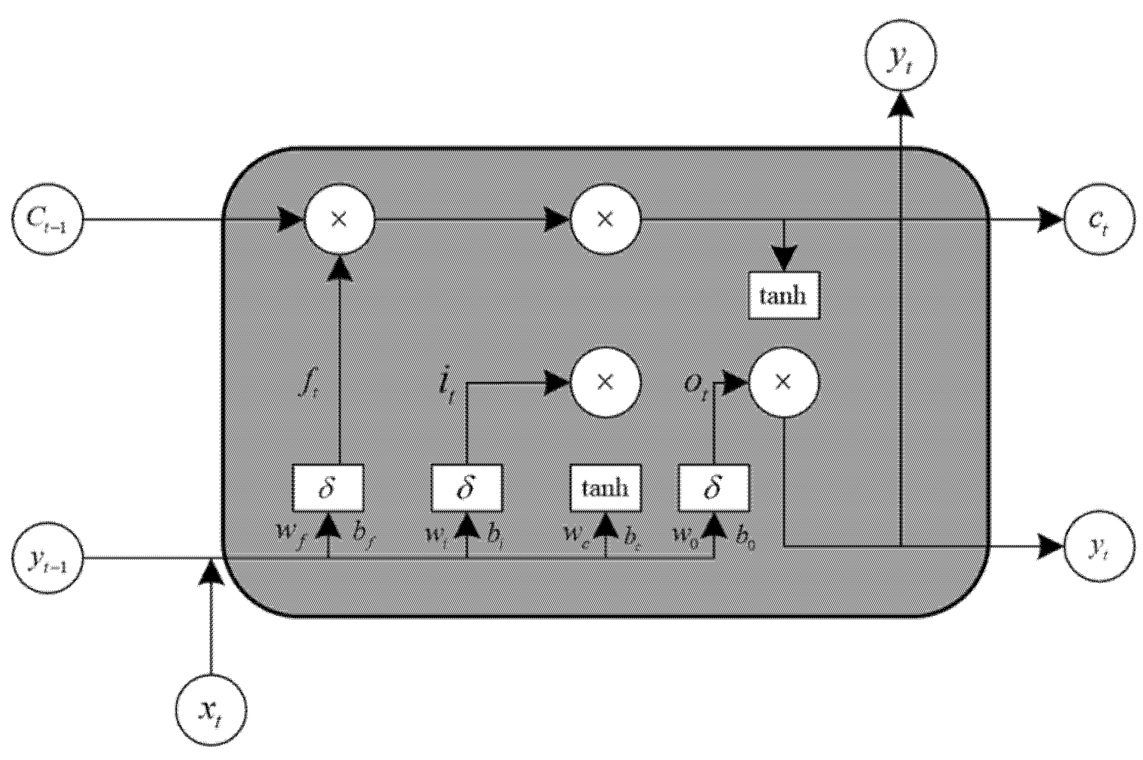
2.1. Long Short-Term Memory Neural Network

Long Short-Term Memory (LSTM), as a special type of Recurrent Neural Network (RNN), uses memory cells instead of traditional neurons in its internal storage units [20,21,22,23]. In addition, LSTM also follows a gate mechanism, which consists of an input gate, a forget gate, and an output gate, enabling LSTM to have the ability to update and control the information flow. LSTM overcomes the shortcomings of RNNs by means of the gate mechanism and memory cells, effectively alleviates the problems of vanishing and exploding gradients, and effectively handles the long-term dependencies in time series data [24]. Figure 2 shows the neural network structure of LSTM.

The gate mechanism of LSTM mainly consists of three gates with different functions. In the figure, $f_t$ represents the forget gate, $i_t$ represents the input gate, $o_t$ represents the output gate, and $\delta$ represents the activation function, which is generally the Sigmoid function.

In the forget gate, the discard $y_{t-1}$ and $x_t$ retention of information in the cell state $C_{t-1}$ at time t − 1 are determined based on the hidden layer. Under the action of the Sigmoid activation function of the forget gate, the output of the forget gate $f$ is within the range of [0, 1], where 0 represents discarding all information about the cell state $C_{t-1}$ at the previous moment and 1 represents retaining all information. The existence of the forget gate enables LSTM to selectively forget and retain some memory contents, thereby avoiding the problems of gradient explosion and gradient vanishing. The expression is as follows:

$$f_t=Sigmoid(w_f\cdot [x_t,y_{t-1}]+b_f)$$

(1)

In the formula, $x_t$ is the input at the current time t, $y_{t-1}$ is the output of the hidden layer at time t − 1, $w_f$ is the weight matrix, $b_f$ is the bias vector, and [] indicates that the variables are connected.

In the input gate, the input gate controls how much input $x_t$ information is added to the cell state $C_t$, and the tanh activation function is also used to update the candidate cell states ${\stackrel{\sim }{c}}_t$. The expression is as follows:

$$i_t=Sigmiod(w_i\cdot [x_t,y_{t-1}]+b_i)$$

(2)

$${\stackrel{\sim }{c}}_t=Sigmoid(w_c\cdot [x_t,y_{t-1}]+b_c)$$

(3)

In the formula, $w_i$ and $w_c$ are the weight matrices, $b_i$ and $b_c$ are the bias vectors.

The cell state $C_{t-1}$ at the previous moment combines with the new candidate cell state ${\stackrel{\sim }{c}}_t$ to update into the new cell state $C_t$, and the expression is as follows:

$$c_t=f_t\cdot c_{t-1}+i_t\cdot {\tilde{c}}_t$$

(4)

In the output gate, the output gate regulates the output of the LSTM unit, selects the valid information in the cell state $C_t$ at the current moment to the cell state at the next moment, and outputs it. The expression is as follows:

$$o_t=Sigmoid(w_0\cdot [x_t,y_{t-1}]+b_0)$$

(5)

$$y_t=o_t\cdot \tanh (c_t)$$

(6)

In the formula, $w_0$ is the weight matrix and $b_0$ is the bias vector.

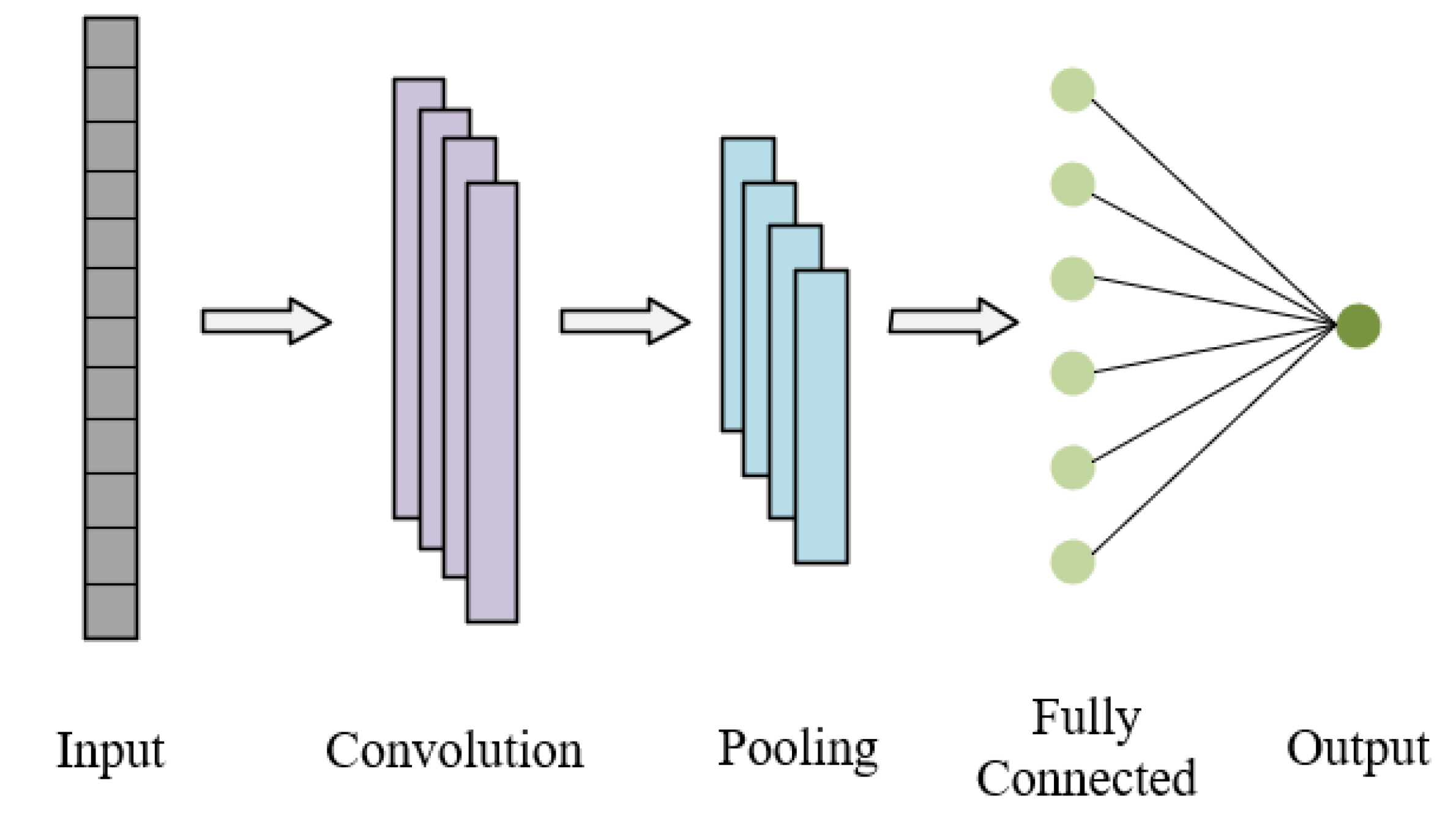
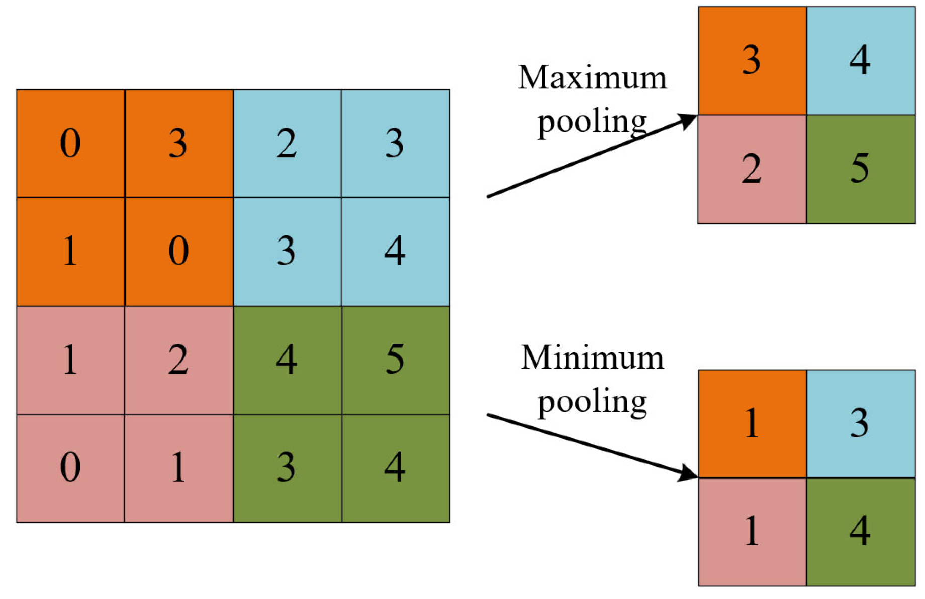
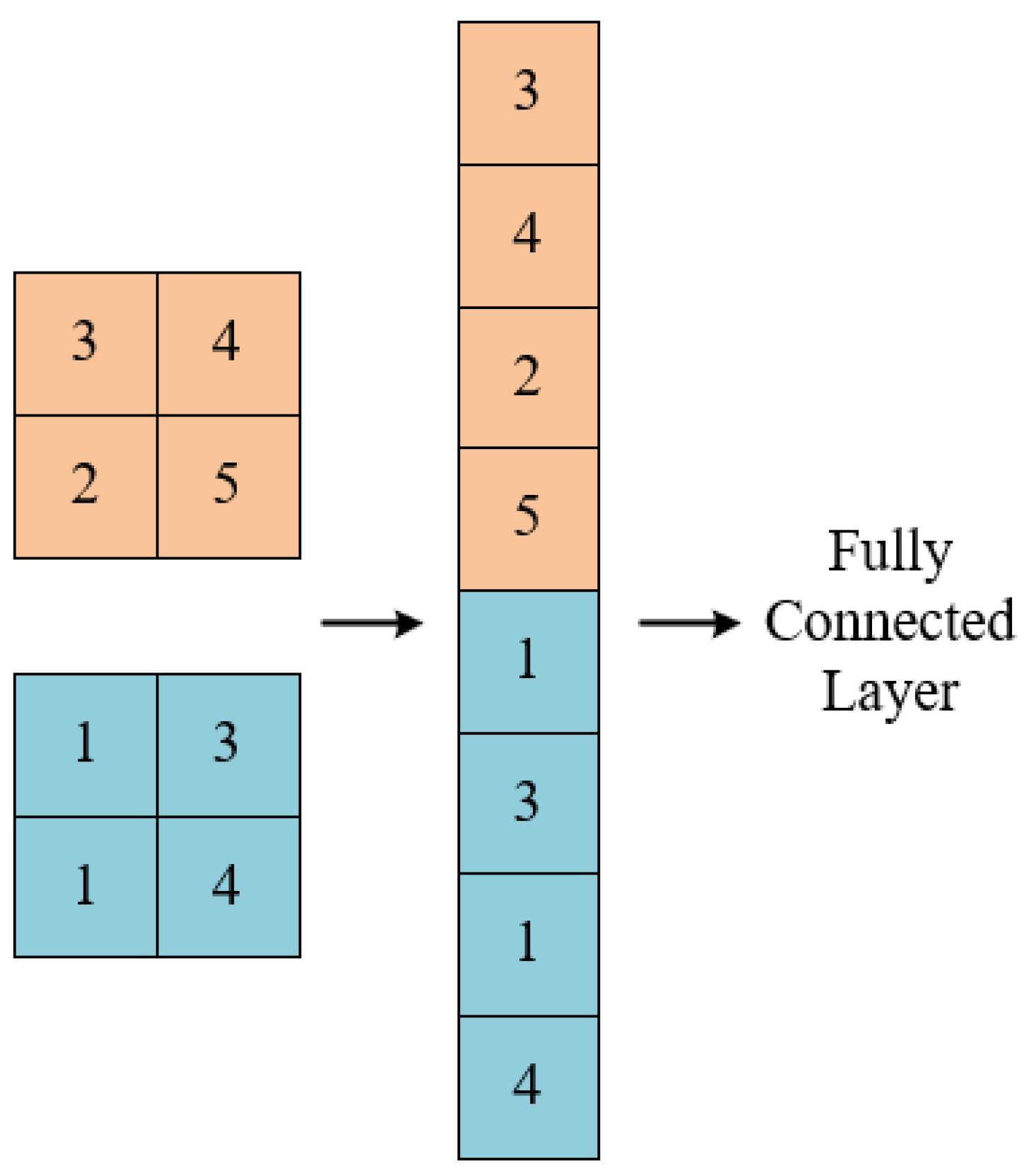
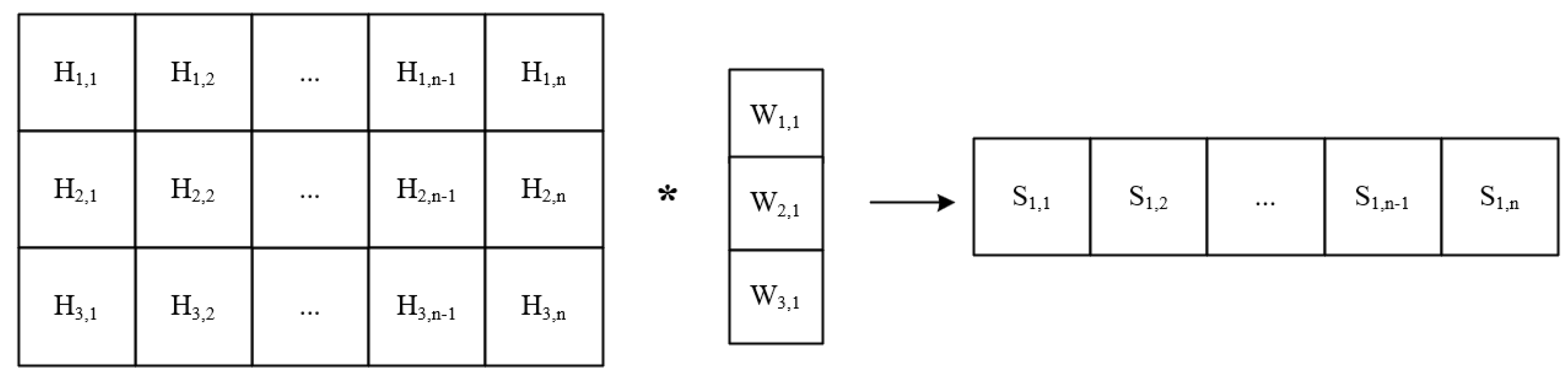
2.2. Convolutional Neural Network

Convolutional Neural Networks (CNNs) belong to an important branch in the development of artificial neural networks and are a kind of feedforward neural network with feature extraction ability and pattern recognition [25,26,27]. In the algorithms of deep learning, compared with other algorithms, CNNs have huge advantages in image processing, object detection, etc. [28]. In recent years, with in-depth research, good achievements have also been made in fields such as natural language processing, signal analysis, and time series. CNNs adopt the methods of local connection and weight sharing to conduct higher-level and more abstract processing on the original data. They can automatically extract the internal features in the data, thereby improving the operational efficiency and performance of the model [29]. As shown in Figure 3, a typical CNN network consists of an input layer, a convolutional layer, a pooling layer, a fully connected layer, and an output layer.

The convolutional layer is an important part of the CNN network. The convolutional layer updates the parameters in the convolutional kernel by using the error backpropagation method and completes the feature extraction of the input matrix through a convolution operation. Convolution kernel size, step size, and filling are three hyperparameters in convolution calculation. The scale of the input matrix should generally be larger than that of the convolution kernel. The smaller the size of the convolution kernel, the fewer the input features that can be extracted. The convolution step size determines the distance that the convolution kernel moves each time it scans the feature map. For example, if the step size is 2, it means that the convolution kernel will skip two pixels in the next scan. The convolution process will lead to the continuous reduction in the size of the feature map, while the filling method can avoid the reduction of the feature map. Suppose the feature map size of the input layer is 4 × 4, the size of the convolution kernel is 2 × 2, the step size is 1, and it is not filled. The convolution calculation process of the neurons in this layer is shown in Figure 4. The green area, for example, is the dot product of the convolution kernel and the corresponding part of the input matrix, and the calculation process is 3 × 1 + 1 × 0 + 5 × 0 + 2 × 1 = 5. In this paper, one-dimensional convolution (Conv1D) is used for feature extraction of sample data.

The purpose of the pooling layer is to perform dimension compression on the convolution data, eliminate invalid information, retain valid information, and accelerate the computing speed. Theoretically, the features after passing through the convolutional layer can be directly used as the input of the fully connected layer. However, the number of features after the convolution operation is huge, which will consume a large amount of computing resources. The further compression of these characteristic quantities by using the pooling layer can effectively reduce the computational load and accelerate the running speed of the model.

The structure of the pooling layer is similar to that of the convolutional layer. The commonly used pooling layer processing mainly includes two methods: maximum pooling and average pooling. Suppose the pooling window is 2 × 2 and the step size is 2. The maximum pooling and average pooling processes are shown in Figure 5. In this paper, one-dimensional Max pooling (MaxPooling1D) is used to compress the dimensions of the sample data.

The fully connected layer (FC) serves as the last layer of the CNN network. Each neuron in this layer integrates local information from the convolutional layer or the pooling layer by connecting with all the neurons in the previous layer. Equations (4)–(7) show the calculation formula of the fully connected layer, where $w$ is the weight matrix, $b$ is the bias vector, $x$ is the input, $y$ is the output, and $f$ is the activation function. Figure 6 shows the full connection process.

$$y(x)=f(w\cdot x+b)$$

(7)

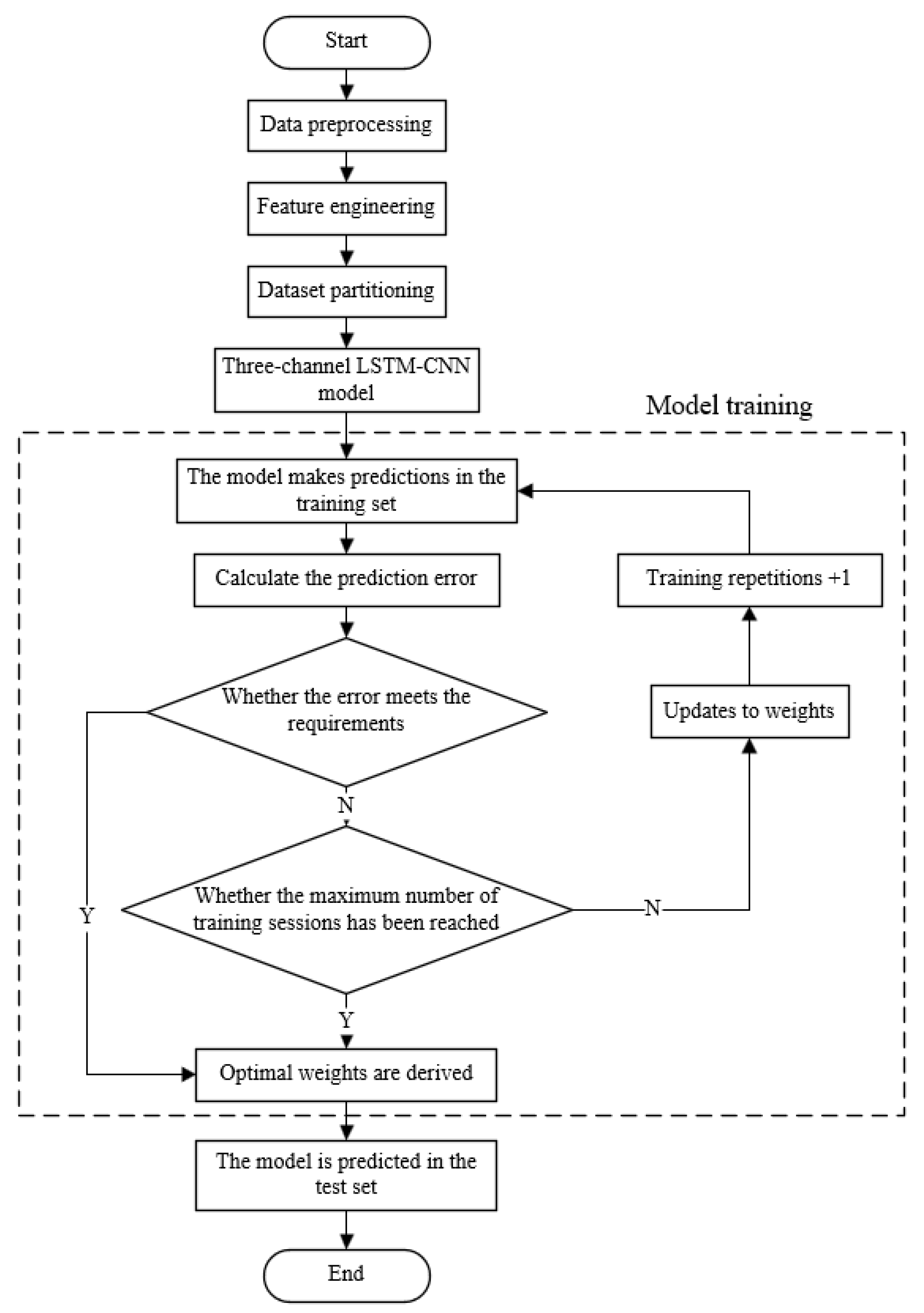
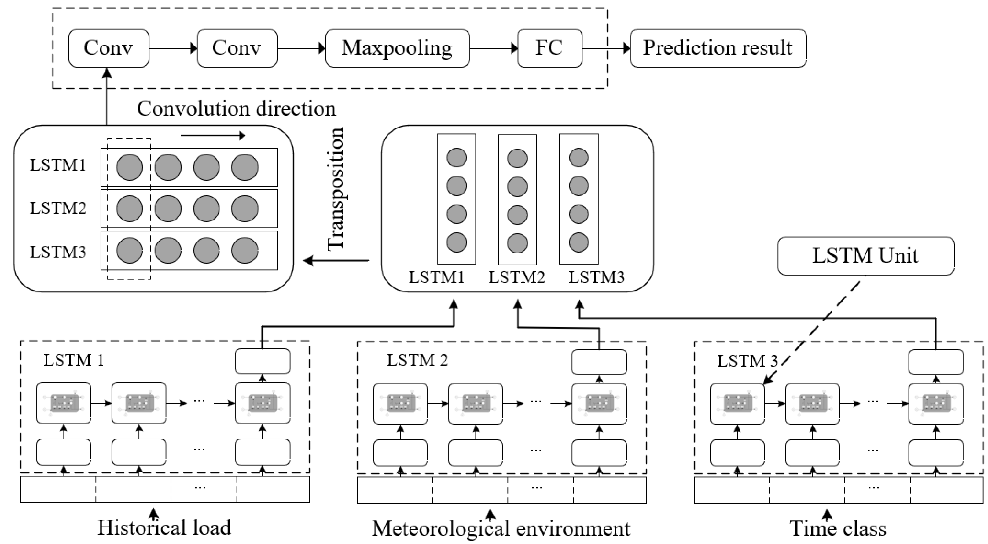
2.3. The Structure of the LSTM + CNN Model with Three Channels of History, Time, and Meteorology

In deep learning, LSTM is widely used in time series analysis due to its advantage of being able to remember historical information for a long time, and CNN has a strong feature extraction ability. The combination of the two has attracted the attention of many researchers, such as CNN-LSTM, because compared with a single model, this kind of combined model is more conducive to improving the prediction accuracy. However, in existing studies, most of them can only predict one load point in the future, which is of little significance in practical applications. In addition, the established models do not fully consider factors such as time and meteorological environment.

Therefore, in order to further deeply explore the intrinsic relationship among temporal characteristics, meteorological and environmental characteristics, historical power load characteristics, and predicted power load and improve the learning ability of the model for various characteristics, this paper proposes a short-term power load prediction model with three channels of the historical, temporal, and meteorological environment, with LSTM + CNN. Firstly, historical data, time data, and meteorological environment data are combined into three LSTM channels to learn the sequence data of history, time and the meteorological environment, respectively. Then, the learning results of these three channels are transposed. Through CNN, these three channels are fused for learning, and the results are predicted to achieve the prediction of power load for the next day.

This model builds three LSTM channels, respectively, for features of different categories, uses a CNN to perform feature fusion on the outputs from different LSTM channels, further explores the intrinsic relationship between various features and power load from the output end, and improves the prediction effect of short-term power load. Figure 7 shows the network structure diagram of the three-channel LSTM-CNN model.

The entire network is mainly composed of three channels of LSTM modules. The inputs of each module are historical power load information, meteorological and environmental information, and time information, respectively. Among them, the historical power load is the power load value at the same time in the days before the prediction date, and the meteorological and environmental information is the characteristics such as temperature and humidity on the prediction day given by the data set. Time information refers to the time of the predicted date, such as months, hours, whether it is a working day, and other characteristics.

The predicted power load point is defined as $X_t$, with $t$ representing the moment of the predicted power load; the input sequence of the historical power load of the LSTM module at the same time m days ago is $\{X_{t-24},X_{t-24*2},\dots ,X_{t-24*\mathrm{m}}\}$, where 24 is the power load value corresponding to each hour of one day. The input sequence of the meteorological environment LSTM module is $\{W_t^1,\dots ,W_t^r\}$, where r represents the total number of meteorological environment features, and W represents the meteorological environment type features. The input sequence of the time LSTM module is $\{T_t^1,\dots ,T_t^e\}$, where T represents the time encoding feature, and e represents the total number of time features. After normalizing each sequence, they are, respectively, sent to the corresponding LSTM modules for sequence learning. Suppose the output of the historical power load LSTM module is $(H_{1,1},H_{1,2},\dots ,H_{1,n})$, the output of the environmental LSTM module is $(H_{2,1},H_{2,2},\dots ,H_{2,n})$, and the output of the time LSTM module is $(H_{3,1},H_{3,2},\dots ,H_{3,n})$, where n is the number of neurons in the LSTM, and the output neurons of each module are concatenated. In order to enable the convolutional network to extract the features of the output neurons of each LSTM module and make them conform to the convolution operation mode in the Tensorflow architecture, in this chapter, the splined neurons are first transposed and then sent to the convolutional network for feature fusion. The convolution process is shown in Figure 8, and the expression is as follows:

$$S_{(1,n)}=f({\displaystyle \sum _{i=1}^3{\displaystyle \sum _{j=1}^n{H}_{(i,j)}\ast w_{(i,j)}+b}})$$

(8)

In the formula, S represents the output after convolution, w is the weight matrix of the convolution kernel, f is the activation function, and b is the bias vector.

In the convolutional network, the features from the output neurons of different modules are first extracted through two layers of one-dimensional convolutional layers (Conv), and the correlation information of various features and power loads is fused. Then, the data dimension reduction processing operation is carried out through the Maxpooling layer to reduce the computational load of the model and improve the running speed. Finally, the dimensionally reduced data is sent into the fully connected layer (FC) to obtain the preliminary power load prediction result. After inverse normalization, the final power load prediction value is obtained.

3. Experimental Parameter Settings

In this paper’s experiment, two power datasets were adopted to verify the performance of the three-channel LSTM-CNN model. One of them was the power dataset of a distribution network in the city of Tétouan, Morocco, for the entire year of 2017. The second one is the dataset of the Electrician Cup competition.

The experimental hardware platform is a notebook computer based on the Windows 11 system, including an Intel Core i5-8300H CPU and an NVDIA GTX 1050Ti GPU. Among them, the software platform is Pycharm (version Community Edition 2024.3.4) based on the python language, and the main development library is the Keras deep learning library based on Tensorflow (version 2.6.0). Keras, as a commonly used framework in deep learning, encapsulates some common deep learning networks, enabling less code to be used for model building in deep learning model construction and making it easier to understand the model-building process.

In the partitioning dataset, the dataset is divided into the training set and the test set. The model is trained in the training set to update the weights and obtain the optimal model and predicted in the test set to obtain the power load prediction results.

In the experiments of this section, batch_size is set to 256. One layer of the LSTM network is set up in each of the three channels, with 64 neurons set up for learning various types of information. In the CNN network, there are 2 convolutional layers and 1 pooling layer. Among them, 8 convolutional kernels are set in the first convolutional layer, and 2 convolutional kernels are set in the second convolutional layer to extract the important feature information in the three-channel LSTM network. The learning rate is set to 0.001, the loss function selects the commonly used MAE loss function in the regression model, and the number of iterations is set to 80.

In neural networks, activation functions are often used to handle nonlinear data, and different activation functions affect the performance of the model. This section sets the activation functions in the proposed network and compares the effects of multiple activation functions on the performance of the model. The experimental results are shown in

Table 1. Comparison of several commonly used activation functions.

Activation Function	RMSE/MW	MAE/MW	MAPE/%
Sigmoid	393.250	315.6	1.155
Tanh	449.462	362.8	1.273
ReLU	651.879	543.2	2.218
Leaky ReLU	321.198	275.3	0.974

. Among several commonly used activation functions, the Leaky ReLU activation function has the best performance and the highest prediction accuracy in the model, followed by the Sigmoid activation function. However, the performance of the ReLU activation function is the worst. Compared with Sigmoid, Tanh, and ReLU, the performance of the Leaky ReLU activation function in MAPE decreased by 0.181%, 0.299%, and 1.244%, respectively. This is due to the special function construction of the ReLU activation function, which leads to the phenomenon that the weights cannot be updated during the gradient calculation process, while the Sigmoid and Tanh activation functions are prone to gradient dispersion problems in the saturation region. The Leaky ReLU activation function sets the slope α within the interval (0, 1) for the input of negative numbers, solving the problems of the inability to update the weights in the ReLU activation function and the vanishing gradient in backpropagation. Therefore, the best-performing Leaky ReLU function is adopted as the activation function.

In the models established in this chapter, the selection of the model optimizer has a certain impact on the model performance. An appropriate optimizer can improve the prediction accuracy of the model. In order to select the appropriate optimizer for the three-channel LSTM-CNN model, this section presents an experimental comparison of two commonly used optimizers. The results are shown in

Table 2. Comparison of different optimizers.

Optimizer	RMSE/MW	MAE/MW	MAPE/%
SGD	523.866	423.7	1.493
RMSprop	335.207	287.5	1.102
Nadam	327.914	280.1	1.038
Adam	321.198	266.4	0.974

. It can be seen that the selection of different optimizers has significant differences in the prediction effect of the model. Among them, the model choosing the Adam optimizer has the best performance. Compared with the SGD optimizer, its prediction accuracy in MAPE has improved by 0.519%. Although Nadam theoretically combines Nesterov momentum with adaptive learning rates, its MAPE increased by 6.2% compared to Adam in our task. This suggests that the standard Adam’s first-moment estimation aligns better with the gradient patterns in multi-channel LSTM-CNN architectures. The RMSprop optimizer showed faster initial convergence but ultimately fell short in handling the coupling effects between temporal and meteorological features. Therefore, in this chapter, the Adam optimizer is selected as the optimizer for the three-channel LSTM-CNN model.

In the three-channel LSTM-CNN short-term power load forecasting model, historical power loads of different lengths affect the model performance. This section conducts an in-depth study on the input length in the historical power load and takes the historical load at the same time from the previous day to the previous four days as the input of the historical load LSTM module, respectively.

Table 3. Performance analysis of different historical load input lengths.

Input Length	RMSE/MW	MAE/MW	MAPE/%
1	321.198	277.1	0.974
2	405.693	338.9	1.130
3	512.023	425.6	1.536
4	1310.602	1005.8	4.520

shows the performance of the model in this chapter under different historical power load input lengths. It can be seen from the table that the MAPE of the model compared with other historical load input lengths has decreased by 0.156%, 0.562%, and 3.564%, respectively. Therefore, in the model of this chapter, the same time of the previous day is selected as the input of the historical load module in the model.

4. Analysis of Experimental Results

In the above-mentioned three-channel LSTM-CNN short-term power load forecasting model experiment, the corresponding parameters of the three-channel LSTM-CNN model were determined. In this section, in order to verify the performance of the short-term power load forecasting model based on the three-channel LSTM-CNN, the Temporal Convolutional Network (TCN), the LSTM model, and the combined model of CNN and LSTM (CNN-LSTM) were adopted as comparison models to verify the prediction effect of the three-channel LSTM-CNN short-term power load forecasting model. The hyperparameters of the LSTM, CNN-LSTM and S-LSTM comparison models were consistent with those of the three-channel LSTM-CNN, and the hyperparameters of the remaining comparison models were selected as the best results after multiple experiments.

(1)

Table 4. Prediction results obtained of different models in the Tétouan City power dataset.

Method	RMSE/MW	MAE/MW	MAPE/%
LSTM	799.783	652.3	1.942
CNN-LSTM	776.214	627.8	1.823
TCN	588.468	492.2	1.471
Three-channel LSTM-CNN	560.581	450.2	1.367

presents the load forecasting results of different models in the Tétouan municipal power supply dataset. It can be known from Table 4 that, compared with the LSTM model, the CNN-LSTM combined model that adds a CNN for feature extraction on the basis of LSTM, and the TCN model, the RMSE of the three-channel LSTM-CNN model decreased by 239.202 MW, 215.660 MW, and 27.887 MW, respectively. MAE decreased by 202.1 MW, 177.6 MW, and 42.0 MW, respectively; MAPE decreased by 0.566%, 0.465% and 0.104%, respectively. It is indicated that the LSTM model after feature extraction using the CNN network can better capture the characteristic information of power load, thereby improving the accuracy of power load prediction. Among all the comparison models, the three-channel LSTM-CNN model has the best effect in power load forecasting. Experiments prove that this model has good predictive performance.

The prediction results of each model in this dataset are shown in Figure 9. Compared with other comparison models, the prediction curve of the three-channel LSTM-CNN model is closer to the change in the real power load, while the prediction effect of the LSTM model is the worst and cannot follow the change of power load well. When some power loads change suddenly, other comparison models are larger than the actual values compared to the three-channel LSTM-CNN. The three-channel LSTM-CNN can better capture the places where the power load suddenly changes and can remain consistent with the changing trend of the power load.

The remaining power load of each model is shown in Figure 10. The majority of the residual power loads of the three-channel LSTM-CNN model proposed in this chapter are less than 1000 kW. Even at some time points where it is difficult to predict accurately due to large fluctuations in power load changes, the residual power load of the three-channel LSTM-CNN model is the lowest among the comparison models. However, the single LSTM model fluctuates the most and has the poorest prediction effect in the variation of the power load residual. The performance of the TCN model is slightly worse than that of the three-channel LSTM-CNN model. The residual variation fluctuation of power load in the three-channel LSTM-CNN model is the most gentle, and the prediction effect of the power load is more accurate.

(2)

Table 5. The prediction results of different models in the Electrician Cup competition dataset.

Method	RMSE/MW	MAE/MW	MAPE/%
LSTM	508.857	407.1	1.522
CNN-LSTM	426.196	343.8	1.246
TCN	358.294	304.7	1.083
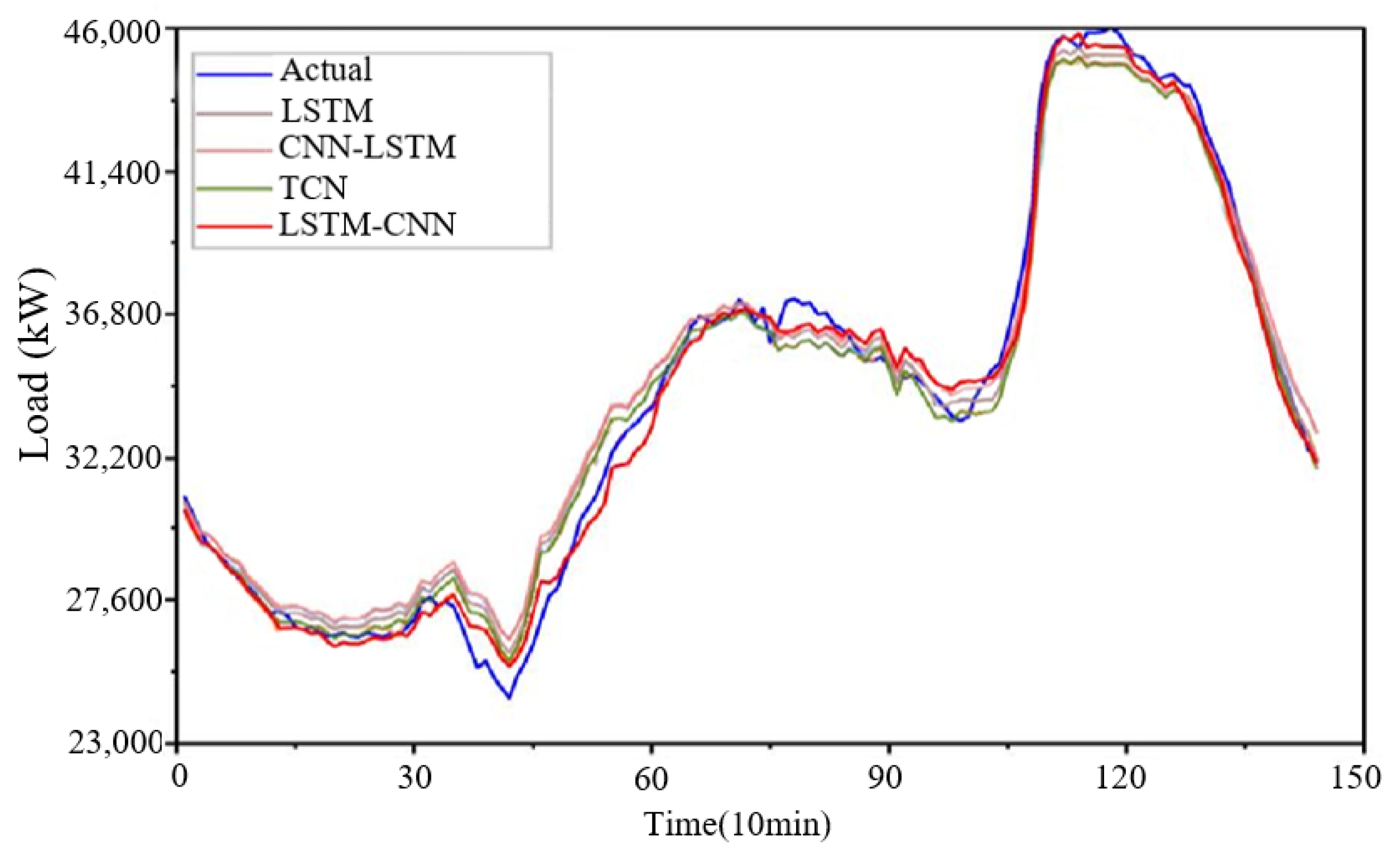
Three-channel LSTM-CNN	321.198	278.6	0.974

shows the load forecasting results of different models in the Electrician Cup competition dataset. It can be known from Table 5 that among the various comparison models, the three-channel LSTM-CNN prediction model has a relatively high accuracy in power load prediction. Its RMSE is 321.198 MW, its MAE is 278.6 MW, and its MAPE is 0.974%. Compared with the LSTM, the CNN-LSTM model, and the TCN model, RMSE decreased by 187.659 MW, 104.998 MW, and 37.096 MW, respectively. The MAE decreased by 128.5 MW, 65.2 MW, and 26.1 MW, respectively. The MAPE decreased by 0.548%, 0.272%, and 0.109%, respectively. All three evaluation indicators decreased, indicating that the model in this section has a good effect on power load forecasting.

The prediction results of each model in the Electrician’s Cup competition dataset are shown in Figure 11, and the comparison of power load residuals of each model is shown in Figure 12. It can be seen from the two figures that in the Electrician’s Cup dataset, the prediction effect of the three-channel LSTM-CNN model is better. It can accurately follow the changes in power load in the morning and evening, and its overall power load residual tends to be more stable. This model can effectively predict the short-term power load of the next day. When the power load is stable and has large fluctuations, its prediction performance and generalization ability show excellent results.

5. Conclusions

This paper proposes a three-channel LSTM-CNN short-term power load forecasting model. The LSTM neural network is utilized to capture the dependency relationships in time series data. Input sequences in different LSTM modules are constructed, respectively, for the characteristics of time information, meteorological environment and historical load to form a three-channel network. Combined with the feature extraction ability of the convolutional network, the output features of each LSTM module in the three-channel network are extracted. Finally, the power load forecasting result is obtained after learning through the fully connected layer.

The experimental results in both datasets show that, compared with various mainstream deep learning models, the prediction performance of the three-channel LSTM-CNN model is better. This proves that this model can effectively fuse features and enhance the correlation between various features and power loads, improving the accuracy of load prediction. In the predicted step size, the three-channel LSTM-CNN model belongs to an improved single-step prediction model. The difference from other single-step prediction models lies in that in the historical load LSTM module of this model, the historical load at the same time of the previous day is adopted as the input, which can correspond to the output of the power load value at the same time in the future. The prediction of all power load points for a consecutive day in the future has been achieved.

References

1. Hao, P.; Yin, S.; Wang, D.; Wang, J. Exploring the influencing factors of urban residential electricity consumption in China. Energy Sustain. Dev. 2023, 72, 278–289. [Google Scholar] [CrossRef]
2. Jiang, Q.; Khattak, S.I.; Rahman, Z.U. Measuring the simultaneous effects of electricity consumption and production on carbon di-oxide emissions (CO2e) in China: New evidence from an EKC-based assessment. Energy 2021, 229, 120616. [Google Scholar] [CrossRef]
3. Hao, Y.; Li, Y.; Guo, Y.; Chai, J.; Yang, C.; Wu, H. Digitalization and electricity consumption: Does internet development contribute to the reduction in electricity intensity in China. Energy Policy 2022, 164, 112912. [Google Scholar] [CrossRef]
4. Zou, H.B.; Yang, Q.H.; Chen, J.T.; Chai, Y.H. Short-term Power Load Forecasting Based on Phase Space Reconstruction and EMD-ELM. J. Electr. Eng. Technol. 2023, 18, 3349–3359. [Google Scholar] [CrossRef]
5. Ji, Y.; An, A.; Zhang, L.; He, P.; Liu, X. Short-term load forecasting based on temporal importance analysis and feature extraction. Electr. Power Syst. Res. 2025, 244, 111551. [Google Scholar]
6. Liu, W.; Li, J. Short-Term Power Load Forecasting Based on Genetic Algorithm Improved VMD-BP. Int. J. Intell. Inf. Technol. 2025, 21, 1–18. [Google Scholar] [CrossRef]
7. Liu, M.; Xia, C.; Xia, Y.; Deng, S.; Wang, Y. TDCN: A novel temporal depthwise convolutional network for short-term load forecasting. Int. J. Electr. Power Energy Syst. 2025, 165, 110512. [Google Scholar] [CrossRef]
8. Chen, W.; Rong, F.; Lin, C. Short-term building electricity load forecasting with a hybrid deep learning method. Energy Build. 2025, 330, 115342. [Google Scholar] [CrossRef]
9. Smyl, S.; Dudek, G.; Pełka, P. Contextually enhanced ES-dRNN with dynamic attention for short-term load forecasting. Neural Netw. 2024, 169, 660–672. [Google Scholar] [CrossRef]
10. Du, S.H.; Gao, T.; Su, J.; Yang, G.; Fang, S. Short-term Load Combination Forecasting Model Based on Causality Mining of Influencing Factors. In Proceedings of the 3rd Asia Energy and Electrical Engineering Symposium (AEEES 2021), Chengdu, China, 26–29 March 2021; pp. 969–973. [Google Scholar]
11. Cheng, L.; Zhang, Y.; Suo, L.; Shen, S.; Fang, F.; Jin, L. Short-Term Cooling, Heating and Electrical Load Forecasting in Business Parks Based on Improved Entropy Method. In Proceedings of the 36th Chinese Control Conference (CCC), Dalian, China, 26–28 July 2017; pp. 10611–10616. [Google Scholar]
12. Chen, X.Y.; Dong, X.L.; Shi, L. Short-Term Power Load Forecasting Based on I-GWO-KELM Algorithm. In Proceedings of the 2nd International Conference on Computer Science Communication and Network Security (CSCNS 2020), Sanya, China, 22–23 December 2020. MATEC Web Conf. 2021, 336, 05021. [Google Scholar] [CrossRef]
13. Zeng, L.S.; Li, Y.L. A Method for Power System Short-Term Load Forecasting Based on Radial Basis Function Neural Network. In Proceedings of the 4th International Conference on Intelligent Systems Design and Engineering Applications (ISDEA), Zhangjiajie, China, 6–7 November 2013; pp. 12–14. [Google Scholar]
14. Giacomazzi, E.; Haag, F.; Hopf, K. Short-term electricity load forecasting using the temporal fusion transformer: Effect of grid hierarchies and data sources. In Proceedings of the 14th ACM International Conference on Future Energy Systems, Orlando, FL, USA, 20–23 June 2023; pp. 353–360. [Google Scholar]
15. Lv, Y.; Wang, L.; Long, D.; Hu, Q.; Hu, Z. Multi-area short-term load forecasting based on spatiotemporal graph neural network. Eng. Appl. Artif. Intell. 2024, 138, 109398. [Google Scholar] [CrossRef]
16. Ren, C.; Jia, L.; Wang, Z. A CNN-LSTM hybrid model based short-term power load forecasting. In Proceedings of the 2021 Power System and Green Energy Conference (PSGEC), Shanghai, China, 20–22 August 2021; IEEE: Piscataway, NJ, USA, 2021; pp. 182–186. [Google Scholar]
17. Zhao, F.; Zhang, C.; Geng, B. Deep multimodal data fusion. ACM Comput. Surv. 2024, 56, 1–36. [Google Scholar] [CrossRef]
18. Zhang, C.J.; Zhang, F.Q.; Gou, F.Y.; Cao, W.S. Study on Short-Term Electricity Load Forecasting Based on the Modified Simplex Approach Sparrow Search Algorithm Mixed with a Bidirectional Long- and Short-Term Memory Network. Processes 2024, 12, 1796. [Google Scholar] [CrossRef]
19. Li, F.; Yu, X.W.; Tian, X.; Zhao, Z.L. Short-Term Load Forecasting for an Industrial Park Using LSTM-RNN Considering Energy Storage. In Proceedings of the 3rd Asia Energy and Electrical Engineering Symposium (AEEES), Chengdu, China, 26–29 March 2021; pp. 684–689. [Google Scholar]
20. Wang, Y.Z.; Zhang, N.Q.; Chen, X. A Short-Term Residential Load Forecasting Model Based on LSTM Recurrent Neural Network Considering Weather Features. Energies 2021, 14, 2737. [Google Scholar] [CrossRef]
21. Yalcinoz, T.; Eminoglu, U. Short Term and Medium Term Power Distribution Load Forecasting by Neural Networks. Energy Convers. Manag. 2005, 46, 1393–1405. [Google Scholar] [CrossRef]
22. Greff, K.; Srivastava, R.K.; Koutník, J.; Steunebrink, B.R.; Schmidhuber, J. LSTM: A search space odyssey. IEEE Trans. Neural Netw. Learn. Syst. 2016, 28, 2222–2232. [Google Scholar] [CrossRef] [PubMed]
23. Mei, T.D.; Si, Z.J.; Yan, J.; Lu, L.F. Short-Term Power Load Forecasting Study Based on IWOA Optimized CNN-BiLSTM. In Advanced Intelligent Computing Technology and Applications, Proceedings of the 20th International Conference on Intelligent Computing (ICIC 2024), Tianjin, China, 5–8 August 2024; Lecture Notes in Computer Science; Springer: Berlin/Heidelberg, Germany, 2024; Volume 14862, pp. 502–510. [Google Scholar]
24. Zhang, W.J.; Qin, J.; Mei, F.; Fu, J.J.; Dai, B.; Yu, W.W. Short-Term Power Load Forecasting Using Integrated Methods Based on Long Short-Term Memory. Sci. China Technol. Sci. 2020, 63, 614–624. [Google Scholar] [CrossRef]
25. Chua, L.O.; Roska, T. The CNN paradigm. IEEE Trans. Circuits Syst. I Fundam. Theory Appl. 1993, 40, 147–156. [Google Scholar] [CrossRef]
26. Dao, F.; Zeng, Y.; Qian, J. Fault diagnosis of hydro-turbine via the incorporation of bayesian algorithm optimized CNN-LSTM neural network. Energy 2024, 290, 130326. [Google Scholar] [CrossRef]
27. Farsi, B.; Amayri, M.; Bouguila, N.; Eicker, U. On Short-Term Load Forecasting Using Machine Learning Techniques and a Novel Parallel Deep LSTM-CNN Approach. IEEE Access 2021, 9, 31191–31212. [Google Scholar] [CrossRef]
28. Yi, S.Y.; Liu, H.C.; Chen, T.; Zhang, J.W.; Fan, Y.B. A Deep LSTM-CNN Based on Self-Attention Mechanism with Input Data Reduction for Short-Term Load Forecasting. IET Gener. Transm. Distrib. 2023, 17, 1538–1552. [Google Scholar] [CrossRef]
29. Agga, F.A.; Abbou, S.A.; El Houm, Y.; Labbadi, M. Short-Term Load Forecasting Based on CNN and LSTM Deep Neural Networks. In Proceedings of the 14th IFAC Workshop on Adaptive and Learning Control Systems (ALCOS 2022), Casablanca, Morocco, 29 June–1 July 2022. IFAC-PapersOnLine 2022, 55, 777–781. [Google Scholar] [CrossRef]
Figure 1. The structure of the model.
Electronics 14 02262 g001
Figure 2. LSTM neural network structure.
Electronics 14 02262 g002
Figure 3. CNN network structure.
Electronics 14 02262 g003
Figure 4. The principle of convolution operation.
Electronics 14 02262 g004
Figure 5. Maximum pooling and average pooling processes.
Electronics 14 02262 g005
Figure 6. Full connection process.
Electronics 14 02262 g006
Figure 7. Three-channel LSTM-CNN combined model structure.
Electronics 14 02262 g007
Figure 8. Convolution operation process.
Electronics 14 02262 g008
Figure 9. Prediction results obtained of the power data set of Tétouan City.
Electronics 14 02262 g009
Figure 10. Analysis of the load residual in the power data set of Tétouan City.
Electronics 14 02262 g010
Figure 11. The prediction results of different models in the Electrician’s Cup dataset.
Electronics 14 02262 g011
Figure 12. Load residuals of different models in the Electrician’s Cup dataset.
Electronics 14 02262 g012