Abstract
Feature selection has been a fundamental research area for both conventional and contemporary machine learning since the beginning of predictive analytics. From early statistical methods, such as principal component analysis, to more recent and data-driven approaches, such as deep unsupervised feature learning, selecting input features to achieve the best objective performance has been a critical component of any machine learning application. In this study, we propose a novel, easily replicable, and robust approach called probability-weighted feature selection (PWFS), which randomly selects a subset of features prior to each training–testing regimen and assigns probability weights to each feature based on an objective performance metric such as accuracy, mean-square error, or area under the curve for the receiver operating characteristic curve (AUC–ROC). Using the objective metric scores and weight assignment techniques based on the golden ratio led iteration method, the features that yield higher performance are incrementally more likely to be selected in subsequent train–test regimens, whereas the opposite is true for features that yield lower performance. This probability-based search method has demonstrated significantly faster convergence to a near-optimal set of features compared to a purely random search within the feature space. We compare our method with an extensive list of twelve popular feature selection algorithms and demonstrate equal or better performance on a range of benchmark datasets. The specific approach to assigning weights to the features also allows for expanded applications in which two correlated features can be included in separate clusters of near-optimal feature sets for ensemble learning scenarios.
1. Introduction
Feature selection is the task of searching for the best features that provide the most information to be used in a prediction or classification problem of large-scale data. Feature selection provides a variety of benefits, such as reduced computational expenses, shorter processing times of large-scale data, better prediction or classification accuracy results in the testing processes, reduced overfitting by the removal of redundant noisy data, and preparing clean, understandable data [1]. It also provides feedback on beneficial features and combinations of features for further data collection in ongoing research projects so that researchers can make more deliberate, informed decisions about data collection points.
Numerous scientific studies entail the meticulous collection of valuable data for the purpose of analyzing diverse hypotheses. Data collection is often both costly and limited in scope, particularly in fields such as the social sciences and consumer research, thereby posing significant challenges for data analytics. In particular, any task employing modern machine learning tools raises a fundamental question: Have the available data been fully leveraged to achieve optimal performance in regression, classification, clustering, or related tasks?
Consider a scenario in which a learning task involves using scientifically collected data as features () to predict an outcome (). When the number of features (j) is significantly large, it becomes impractical to perform a complete combinatorial analysis of all possible combinations of features using empirical training/test/validation cycles. In such cases, most feature selection algorithms rely on statistical analyses of the feature space to identify and eliminate correlations, aiming to boost performance.
In this article, we propose a novel approach that differs fundamentally from existing methods. Instead of relying solely on statistical analysis, we probabilistically sample the feature-performance space to empirically approximate the maximum achievable performance from the available data. To our knowledge, our method is unique in the way it approximates the ideal, yet computationally infeasible, combinatorial search space, focusing on its higher-performing regions in terms of accuracy.
We demonstrate across a range of datasets that, compared to commonly used feature selection algorithms, our approach achieves equal or superior performance. Moreover, it preserves a process flow that closely approximates the ideal feature selection from an otherwise impossibly large combinatorial search space.
2. Relevant Work
There exists a variety of feature selection algorithms, conventional, statistical, wrapper, and embedded model-based, which have been accepted into the literature. We implemented these methods to obtain a comparison with the method we propose in this research, PWFS.
Mutual information (MI) detects relationships and dependencies between datasets involving mean values, variances, higher moments, or any other statistical aspects of the data. There are a variety of units that represent this information, such as bits (Shannon), nats, or hartleys, depending on the logarithmic base used in the calculation. The distribution properties of the data, i.e., their entropy values, are estimated with the help of k-nearest neighbors, contributing to the robustness of the mutual information calculation.
Equation (1) shows the mutual information of X,Y; where X,Y are two random variables, is the probability measure for X and Y, and and are the marginal density functions for X and Y [2]. If the random variables X and Y were independent, i.e., completely uncorrelated, the would result in ; therefore, the MI of I(X;Y) would result in zero.
Mutual importance is a greedy forward stepwise, uni-variate filtering method. This means that the importance of each feature is calculated individually, and features are selected incrementally, one feature at a time, rather than a combinatorial approach. Higher values of mutual information indicate a stronger relationship or dependency between the variables. Zhou et al. offered a feature selection method based on mutual information along with correlation coefficient (CCMI) in order to remove more redundant information in the evaluation criteria [3].
The Fisher score for each feature is computed using the ratio of the between-class variance to the within-class variance. Fisher scores for all features are calculated and then ranked. The Fisher score evaluates features individually and cannot handle feature redundancy. This method is used for dimensionality reduction by selecting the features that rank highest [4]. Lin Sun et al. used the Fisher score method to eliminate irrelevant genes to significantly reduce computational complexity, tasked with evaluating features for tumor classification [5]. Sun et al. proposed a filter-wrapper preprocessing algorithm for feature selection, employing an improved Fisher score model to reduce the spatiotemporal complexity of multi-class data, and designed a heuristic feature selection algorithm to improve classification performance on multi-class datasets [6].
ANOVA, or analysis of variance, is a statistical method used to assess whether the means of two or more groups are significantly different from each other. The ANOVA F-value is a statistic calculated in the context of ANOVA and is used to test the null hypothesis that the means of several groups are equal. Shakeela et al. used analysis of variance (ANOVA) with F-statistics computations to choose distinctive features in network traffic data [7]. Jamil et al. presented the influence of the one-way ANOVA feature-ranking technique on the performance of four ML classifiers, namely the decision tree, SVM, KNN, and ANN for fault classification in a ball bearing [8].
Sequential feature selection is a method in which the estimator model either chooses and keeps the most significant feature (FSFS, forward sequential feature selection) or removes the least significant feature (BSFS, backward sequential feature selection) from the data frame depending on the prediction performance at each training and testing iteration of the model using all the data. This process is repeated until the desired number of features has been selected. Aggrawal, R. and Pal, S. used this method to improve the accuracy of diagnosing heart disease, where their experimental results show that the random forest classifier, along with the SFS method, reaches higher accuracy compared to traditional feature selection methods [9].
Recursive feature elimination (RFE) selects features by recursively considering smaller and smaller sets of features. The estimator is trained on the initial set of features, and the importance of each feature is obtained either through any specific attribute such as weights assigned to the feature (coef_) or feature importance object (feature_importances_), which is calculated by the estimator model. Given that our model uses random forest as the estimator, the feature importance metric is defined by the frequency of the feature’s usage at split points of a random forest tree. The least important features are pruned from the current set of features. This procedure is recursively repeated on the pruned set until the desired number of features to be selected is finally reached. RFE was initially proposed to allow support vector machines to perform feature selection by iteratively training a model, ranking features, and then removing the lowest-ranking features [10]. More recently, Sharma et al. proposed a model based on deep reinforcement learning and feature selection through the recursive feature elimination method for effective intrusion and cyber threat detection. With recursive feature elimination, they improved computational costs by reducing the number of features, making the model more efficient compared to traditional methods [11].
SelectFromModel is a meta-transformer executed in embedded feature selection methods. It can be used alongside any estimator that assigns importance to each feature through a specific attribute (such as coef_ or feature_importances_) or via an importance_getter callable after fitting. The training and feature importance association is not recursive, meaning that feature importances are not reassigned iteratively over multiple training sets. The features are considered unimportant and are removed if the corresponding importance values of the features are below the provided threshold parameter. In combination with the threshold criteria, one can use the max_features parameter to set a limit on the number of features selected. Liu et al. used an embedded feature selection method using their proposed weighted Gini index (WGI) to choose a subset of features that favor the accurate determination of the minority class in imbalanced datasets [12].
Boruta is a wrapper-based feature selection method that evaluates feature relevance by leveraging an external estimator, typically a random forest. Unlike embedded methods, which perform selection during model training, Boruta operates independently of the training process. It works by iteratively augmenting the dataset with shadow features, i.e., randomly shuffled copies of original features that serve as a baseline for comparison. In each iteration, a random forest model is trained on the extended dataset, and feature importance scores are computed. Boruta then compares the importance of each original feature to the maximum importance score achieved by any shadow feature. A feature is considered important if it consistently outperforms the shadow features across multiple iterations. The algorithm outputs a list of accepted (important) features for downstream analysis, and this number can be higher than the exact number of features that we are looking for. For ranking these selected features, we subsequently use the feature_importances_ attribute of the random forest model to determine the top seven features. Zhou et al. demonstrated the utility of Boruta in a medical context by integrating it with ensemble models to predict diabetes, where the algorithm successfully reduced dimensionality while retaining predictive power [13].
The ReliefF algorithm is a widely used feature selection method that estimates the importance of features based on their ability to differentiate between instances of different classes while accounting for local data structures. For each randomly selected instance, ReliefF identifies its nearest neighbors from the same class (hits) and from other classes (misses), then updates feature weights by rewarding those that show large differences between the instance and its misses and penalizing those with large differences from hits. This process is repeated for a number of iterations, and the resulting feature weights reflect the relevance of each feature in separating classes. ReliefF supports multiclass classification and is more robust to noisy data and feature interactions. Its effectiveness has been demonstrated in various domains, including sound-based degradation diagnosis of railway point machines [14] and signal-based fault classification in electrical systems [15].
The least absolute shrinkage and selection operator (Lasso) is a regression-based feature selection technique. Lasso works by adding an L1 penalty term to the loss function, which forces the coefficients of less important features to shrink toward zero. This property effectively eliminates irrelevant or redundant features, making Lasso particularly valuable when dealing with high-dimensional datasets. It has been widely adopted in various domains, including biomedical data analysis and engineering applications. For example, Lasso was successfully used in feature selection for enhanced fault diagnosis and classification in bearings [16].
SHAP (Shapley additive explanation) values are feature importance metrics that are tied to the prediction outcome of the machine learning model. These values provide the contribution of each feature to the prediction [17]. They are based on the "players" in coalitional game theory and are used to increase the transparency and interpretability of machine learning models. Players can select individual features or a coalition of features of a data instance. To compute Shapley values, the algorithm simulates that only some feature values are “present”, and some are “absent” in such a way that, in game theory, a player can join or not join a game. Lee et al. conducted SHAP value analysis, a method in explainable AI, to assess the importance of features in the Korea Power Exchange data used for training a load forecasting model [18].
Our study presents an innovative, simple-to-replicate, and resilient method termed probability-weighted feature selection (PWFS). This technique randomly chooses a group of features before each training and testing cycle and assigns probability weights to each feature according to an objective performance measure, such as accuracy, mean squared error, or area under the curve for the receiver operating characteristic curve (AUC–ROC). The next section will describe the operational characteristics of the proposed method, followed by a brief description of the benchmark datasets and comparative results with the previously described literature. The paper will conclude with a discussion of the results and a comprehensive future work on how the algorithm can be improved or applied to other learning schemes, such as ensemble learning.
3. Methodology
PWFS (probability-weighted feature selection) is a model-driven empirical approach to feature selection tasks. It offers an advantage by revealing the overall pattern of performance enhancements when features are randomly combined. This allows the identification of the best performing feature set with a higher level of confidence compared to a completely random approach, which does not guarantee optimal results across multiple attempts.
A simplified overview of the PWFS method is presented in Figure 1. The idea behind PWFS is to assign importance weights to randomly selected features and iteratively make more educated, randomized feature selections. The dataset comprising the selected features is trained and tested using the predefined machine learning mode and is evaluated over performance metrics, accuracy, and AUC–ROC. There can be different methods for the initialization and calculation of these weights of the features, which are controlled by the hyperparameters of PWFS. The learning rate, trial count, number of features, slots, slotting method, slot resetting, and different weight equations are some of the hyperparameters used for settings and initializations. The estimator model to be used in the selection of top-performing features is also a parameter of the PWFS. The user can define a custom estimator and determine its function within the PWFS algorithm.
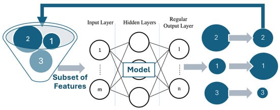
Figure 1.
Overview of the PWFS method.
The probability of selecting each feature is based on its weight relative to the total weight of all features. The probability of selecting a particular feature with weight is provided by Equation (2).
where P(i) is the probability of selecting feature i, and is the weight of feature i. This equation essentially normalizes the weights so that the probabilities sum to 1, ensuring that the sampling process is based on a valid probability distribution. The DataFrame sampling function aligns the weights with the target data based on index values when it is provided with a series as weights. If the weights do not sum to 1, they are automatically normalized to do so. Any index in the weights that does not exist in the DataFrame is ignored.
A detailed flowchart of the PWFS method is presented in Figure 2.
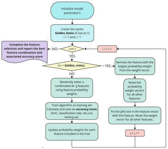
Figure 2.
Flowchart of the PWFS algorithm.
An explanation of the algorithm flowchart is presented below:
- The first step is the initialization of PWFS parameters, which include the following:
- -
- The number of features to be selected f out of n features in the dataset;
- -
- The total number of trials for which the algorithm will evaluate features, ML
- -
- The ML model to be used with PWFS;
- -
- Initialization of the base weights corresponding to the features to create the weight vector ;
- -
- The method to assign weights to the features, i.e., weight equation selection;
- -
- The constant that governs the pace of the weight update (learning rate, );
- -
- Whether the slotting algorithm is going to be executed;
- -
- If the slotting algorithm is used, the type of slotting algorithm.
- In the next step, if enabled, the slotting method subroutine is determined, along with its initialization parameters: the number of trials and the number of features.Using the golden ratio (GR) slotting subroutine, we create an array of Fibonacci series (F) using Equation (3) and then use this array in our GR calculations in Equation (4):The idea behind using the GR is to have a larger number of trials in the first slots in order to reassess the base weight values, comparing them to most of the features of the dataset. The GR subroutine returns an array that is the length of the total number of features to be selected and is created by partitioning the total number of trials into individual slots assigned to each of these features.
- Execute PWFS until the trial number is met. Report the best combination of features and associated accuracy score.
- If a slot has ended,
- -
- select the best feature using the maximum weight in the weights vector;
- -
- store it in the array of selected features and remove it from the weight vector as well as the remaining features of the dataset;
- -
- decrement the number of features to be sampled further on;
- -
- reset the probability weight vector for all remaining features.
- Sample a combination of features and construct a subset that includes both the newly selected and previously chosen features. For each trial, use 10-fold cross-validation (CV), where the algorithm is trained and tested on separate folds and the accuracy score is averaged over all folds. The CV loop is omitted from the flowchart to ensure clarity for the steps of the proposed algorithm.
- Update the weights of the features that were sampled using the predefined weight update method.
- End trials once the total trial number is met.
We explored three different weight-calculation methods and embedded these equations as options in the code of PWFS. These equations calculate the new weights to be assigned to the features and are influenced by statistical methods such as step size calculations in gradient descent and mean deviation.
Weightage1 calculates new weights using Equation (5):
where ACCALL is the average of all of the test accuracy scores.
Weightage2 calculates new weights using Equation (6):
where ACCCOMB is the average of all of the test accuracy scores achieved with the current features in the selected combination.
Weightage3 calculates new weights using Equation (7):
where ACCIND is the average of the test accuracy scores associated with each feature, which are acquired every time a specific feature is used during the trials until the current trial.
The calculated new weight vector is input into the sampling function, where the features of the dataset are randomly sampled.
The method for separating the most efficient features and forcing these features to be utilized in the remaining random sampling processes iteratively is an option called “Slot”. The user may also specify the number of trials for which ’slotting’ is performed, as well as whether the weights should be reset to their initial values after each slotting instance. Figure 3 represents the feature selection task of the Turkish Music Evaluation Dataset using the PWFS method but without any slotting method applied.
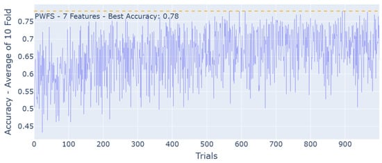
Figure 3.
PWFS log results for the Turkish Music Evaluation Dataset without the slotting algorithm. The most significant features are 3, 19, 20, 23, 32, 35, and 46.
We explored two different predetermined methods for slotting in PWFS. For both of these methods, the last slot of the feature selection is defined to go through all of the remaining features that were not selected in the prior slots rather than a random sampling process and find the most significant, informative last feature depending on the performance metric. Linear slotting simply divides the number of trials by the number of features to be selected in a linear, equal fashion and assigns this number to each slot. Figure 4 represents the linear slotting for the feature selection task of the Turkish Music Evaluation Dataset using the PWFS method. The golden ratio slotting method uses the Fibonacci series to create an approach with larger slots in the first trials of PWFS to provide an “equal opportunity” for the features to be selected so that a better base can be achieved. Figure 5 represents “Golden Ratio” slotting for the feature selection task of the Turkish Music Evaluation Dataset using the PWFS method. Golden ratio slotting was proven to provide better feature selection and, thus, improved accuracy results compared to linear slotting. This trend was observed across other datasets considered in this paper.
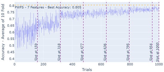
Figure 4.
PWFS log results for the Turkish Music Evaluation Dataset with the linear slotting algorithm. The weights are reset after each slot. The most significant features are 3, 19, 20, 25, 30, 46, and 49.
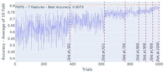
Figure 5.
PWFS log results for the Turkish Music Evaluation Dataset.
Resetting the weights after each slot helps eliminate the likelihood of highly correlated features being selected in the combinations. For instance, in this case, we have two highly correlated features that provide higher prediction accuracy when selected within combinations individually. We can expect a lower prediction accuracy when both of these features are selected. On the other hand, their weights will increase throughout the iterations, where these features are selected individually. After the slot ends and one of the features is selected, by resetting the weights of the remainder of the features, we decrease the chance of the second correlated feature being selected as well. Figure 6 represents the PWFS linear slotting algorithm without weight resets after each slot for the Turkish Music Evaluation Dataset. The intercorrelations of the features selected by PWFS by resetting the weights after each slot vs. not resetting the weights are displayed in Table 1. The correlation values are the absolute averages for the seven features selected by PWFS. It can be observed that the features selected while resetting the weights in each slot have less correlation compared to the features selected without resetting the weights.
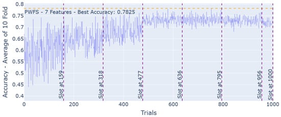
Figure 6.
PWFS log results for the Turkish Music Evaluation Dataset with the linear slotting algorithm. The weights are not reset after each slot. The most significant features are 1, 17, 18, 21, 30, 44, and 47.

Table 1.
Intercorrelations of selected features depending on the slotting methods used.
Applications of different slotting methods, such as adaptive, dataset-driven slotting, are a part of the future research of the PWFS project.
Adaptive slotting is a technique we developed to reduce the processing time of the PWFS algorithm. It operates by invoking a subroutine that dynamically monitors the weights assigned to individual features and identifies dominant features. This identification is achieved by comparing each feature’s weight to the median of the overall weight vector. If a dominant weight is detected, i.e., a feature whose weight significantly exceeds the median, the algorithm terminates the current slot early (i.e., it cuts short the number of trials originally allocated to that slot). After the slot is shortened, the user-defined slotting method (e.g., golden ratio or linear) is reapplied to generate a new slot location array for the remaining trials and features to be selected. This process continues iteratively, allowing the algorithm to focus computation on more informative features while skipping over less relevant ones earlier. A comparison of the slotted, non-slotted, and adaptive slotted performance for the Turkish Music Evaluation Dataset is displayed in Figure 7.
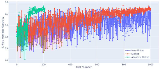
Figure 7.
Comparison of slotted, non-slotted, and adaptive slotted performance for the Turkish Music Evaluation Dataset.
The trial count is the number of trials for which the best features would be searched. The PWFS will continue the trials until the number of features asked has been met. In each trial, the learning rate will update the weights, which is another hyperparameter where the user can define how aggressively they want to update the weights.
At each trial, a new sub-dataset is formed using the features selected. This new sub-dataset consists of all of the instances of the initial dataset. The PWFS algorithm aims to find the best features for the selected machine learning model; therefore, a model must be defined prior to using the PWFS algorithm. PWFS trains and tests this dataset using the predefined model in a K = 10-fold fashion. The average test accuracy result of the folds is calculated and saved to be used as a metric in the calculations of the weights to be assigned to the features. This process is repeated until the trial number meets the slot number, assuming the slotting algorithm is executed. The feature with the highest weight is selected to be used in all of the feature combinations in the remaining trials. This procedure proceeds until the very last feature is selected. The PWFS algorithm scans through all of the remaining features, evaluates the estimator model, and settles on the best-performing feature after going through all 10 folds.
PWFS works on the combinatorial search of the features, which is another advantage over sequential feature selection methods. Sequential selection methods seek the most efficient individual features on a cross-validated model–data pair. The features selected in this method can be highly correlated and may cause diminished performance when selected as the best feature set for testing purposes.
4. Results
Each of the feature selection methods described in Section 2 is employed to identify the optimal combination of seven features using the datasets presented in Table 2.
Table 2.
Datasets used in the research.
The Turkish Music Emotion Dataset is structured as a discrete model and comprises four classes: happy, sad, angry, and relaxed. To prepare the dataset, both verbal and non-verbal music selections were made from various genres of Turkish music [19]. Features are continuous variables that represent acoustic musical properties such as tempo, fluctuation mean, harmonic change detection, chromatogram mean, spectral flatness mean, etc.
The QSAR Biodegradation Dataset was built by the Milano Chemometrics and QSAR Research Group [20]. The features represent 41 molecular descriptors and the physicochemical properties of the materials and molecules. The label column classifies the molecule as ready biodegradable (RB) or not ready biodegradable (NRB).
The Spambase dataset is a categorical dataset of email characteristics and a label column that classifies whether the email was considered spam or not [21]. The features consist of integer or real values that quantify properties such as the frequency of specific words or characters in an email, as well as run-length attributes that measure the length of sequences of consecutive capital letters.
The Steel Plates Faults Dataset classifies the seven types of steel plate faults [22]. The 27 independent features represent physical properties such as the luminosity, type of steel, edges, and orientation index, which are integer and real values.
To prepare the datasets, the MinMaxScaler from the Scikit-learn preprocessing library was used. MinMaxScaler scales and translates the values of each feature based on the specified minimum and maximum values, typically zero and one. Each feature in the dataset is individually rescaled to fit within its corresponding range.
Each of the conventional feature selection methods was implemented using K-fold cross validation. The methods run and return the most important features K = 10 times, each time using a different nine-fold set for training and a different fold for testing. We kept K = 10 constant across all of the traditional methods throughout testing on different datasets to obtain a better comparison. The most important features selected by the methods used were determined after analyzing the folds using the total occurrence count of the features. For instance, 10-fold feature selection using the RFE method is represented in Table 3. The features selected for the method were 1, 12, 22, 27, 34, 36, and 39.
Table 3.
QSAR Biodegradation Dataset: 10-fold representation of the features selected in each fold using the recursive feature selection method.
Datasets assembled using the selected seven features by each of the conventional methods were then used again to train and test a random forest model using the K = 10-fold convention. The accuracy scores of each method were obtained by averaging the accuracy score of the folds.
As provided in Table 4, six of the features selected by PWFS (3, 20, 23, 25, 46, and 49) were also selected by at least one of the conventional feature selection methods, as highlighted in bold font.
Table 4.
Turkish Music Emotion Dataset. Best features: the selection of the top-7 features using different techniques.
The features selected by the K = 10-fold implementation of the conventional feature selection methods, as well as the offered method PWFS, are studied and compared.
As observed in Table 4, the highest accuracy achieved in training and testing the Turkish Music Emotion Dataset, using only the features selected by the corresponding method, was 0.8075 with PWFS, as presented in this study. PWFS resulted in a 12.5% reduction in the error rate compared to the second-best feature selection method, FSFS, which provided an accuracy score of 0.78. BSFS, which is another sequential feature selection method with only the direction difference from FSFS, provided the third-best accuracy score: 0.775.
The increment in the accuracy results, as the PWFS algorithm is searching through the feature sets of the Turkish Music Emotion Dataset and establishing base features with each slot, can be seen in Figure 5.
The comparison of the feature selection method applied to the QSAR Biodegradation Dataset is represented in Table 5. For the QSAR Biodegradation Dataset, the algorithms that provided better results over the rest of the feature selection methods were BSFS and PWFS, with accuracy results of 0.8748 and 0.8730, respectively. PWFS yielded results that are highly comparable in performance to conventional methods on the QSAR Biodegradation Dataset.
Table 5.
QSAR Biodegradation Dataset. Best features: The selection of the top-7 features using different techniques.
The increment in the accuracy results, as the PWFS algorithm is searching through the feature sets of the QSAR Biodegradation Dataset and establishing base features with each slot, can be seen in Figure 8.
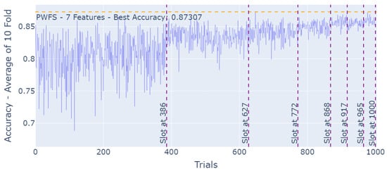
Figure 8.
PWFS log results for the QSAR Biodegradation Dataset.
The accuracy results observed by each of the feature selection methods for the Spambase Dataset are represented in Table 6. Similar to the QSAR Biodegradation Dataset, PWFS and the sequential feature selection methods competed for the best-performing method. FSFS leads the three with a 0.9261 accuracy score, followed by PWFS with 0.9254, which is a scientifically insignificant difference. What is interesting to see here is that although these methods provide almost the same result, the features they used in order to accomplish these scores are 28% different. FSFS picked features 19 and 27, whereas PWFS picked features 21 and 25.
Table 6.
Spambase Dataset. Best features: The selection of the top-7 features using different techniques.
The increment in the accuracy results, as the PWFS algorithm is searching through the feature sets of the Spambase dataset and establishing base features with each slot, can be seen in Figure 9.
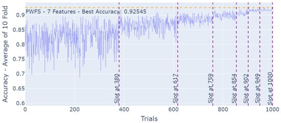
Figure 9.
PWFS log results for the Spambase Dataset.
The accuracy results of the training and testing of the datasets formed by the features of the Steel Plate Faults Dataset using conventional feature selection methods as well as PWFS are represented in Table 7. Here, PWFS provides the best accuracy score of 0.8181, followed by BSFS with 0.7985. These two algorithms used only three common features to accomplish the highest accuracy scores.
Table 7.
Steel Plates Faults Dataset. Best features: The selection of the top-7 features using different techniques.
The increment in the accuracy results, as the PWFS algorithm is searching through the feature sets of the Steel Plates Faults Dataset and establishing base features with each slot, can be seen in Figure 10.
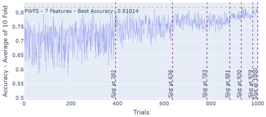
Figure 10.
PWFS log results for the Steel Plates Faults Dataset.
5. Discussion: Training Speed and Accuracy Trade-Off
In many real-world scenarios, particularly in specialized scientific or industrial domains, the process of data collection can be highly resource-intensive, both in terms of time and cost. For example, datasets derived from clinical trials, geological surveys, or long-term monitoring of physical systems may take months or even years to gather. In such cases, where the availability of data is constrained, and each feature or instance is valuable, the emphasis naturally shifts toward maximizing the utility and performance of any subsequent analysis.
Within this context, it becomes evident that computational trade-offs, such as longer feature selection or model training times, are often justifiable. Although certain feature selection methods may significantly reduce the processing time, they often yield lower-performing models due to their more straightforward, statistics-based exploration of feature interactions and contributions. In scenarios where even marginal improvements in accuracy can translate to more reliable predictions or deeper scientific insights, a delay of several minutes, or even hours, is a reasonable cost.
Therefore, it is essential for researchers to prioritize methodological rigor and model performance over minor computational delays, especially when working with datasets that are difficult to acquire or replicate. The goal should be to ensure that the final model extracts as much predictive power and interpretive value as possible from the available data, making the most of what is often a rare and non-renewable resource.
In the context of feature selection, increasing the number of features that effectively capture and span the data space can enhance a model’s ability to accurately represent the underlying data distribution. However, this must be balanced against potential drawbacks such as overfitting, increased computational cost, and reduced interpretability. In this study, a fixed number of seven features was used across all selection methods to provide a fair and standardized basis for comparing model performance. This number was selected as a trade-off large enough to retain critical information from the dataset yet small enough to promote model simplicity and limit redundancy.
As reflected in the seven-feature results tables, the highest-performing methods frequently converge on a core set of three to four common features. This indicates the presence of a dominant subset of features with strong discriminative power. The remaining selected features appear to play a more supportive role, offering marginal gains in performance. As additional supportive features are introduced, the performance improvements across models begin to converge. This convergence implies diminishing returns from further feature selection, particularly when the variance in the importance of the remaining features becomes minimal. To further explore this effect, we conducted additional performance evaluations using the best-performing methods while limiting the number of selected features to 3, 4, and 5, also monitoring the associated computational costs. The results are provided in Table 8, Table 9, Table 10 and Table 11.
Table 8.
Turkish Music Dataset: Comparison of feature selection methods on accuracy and runtime.
Table 9.
QSAR Biodeg Dataset: Comparison of feature selection methods on accuracy and runtime.
Table 10.
Spambase Dataset: Comparison of feature selection methods on accuracy and runtime.
Table 11.
Steel Plates Dataset: Comparison of feature selection methods on accuracy and runtime.
Our experiments showed that probability-weighted feature selection (PWFS) required longer computation times compared to simpler methods like SHAP, sequential feature selection, or filter-based approaches. For instance, PWFS frequently had the highest time cost but also consistently delivered the best accuracy across all datasets. In the final benchmark, PWFS achieved an accuracy of up to 0.8220, outperforming other techniques by a noticeable margin. The time is much higher compared to SHAP and FSFS due to the progressive nature of the method, which requires multiple iterations to build upon previously selected features. However, compared to the alternative, i.e., combinatorial search, this still is a fraction of the time needed to comb the entire search space.
Although most feature selection algorithms require the number of selected features to be predefined as a hyperparameter, our proposed algorithm introduces flexibility by adaptively determining when to stop the selection process. The iterative nature of our method allows us to construct a dynamic data frame that tracks feature weights at each step. This enables real-time analysis of feature importance and facilitates the implementation of an adaptive slotting mechanism. Inspired by this approach, the algorithm can monitor the variance in feature weights, and when this variance diminishes, indicating that additional features contribute comparably less, the algorithm can trigger an early stopping criterion to suggest an appropriate number of features. A promising direction for future work is to further develop this capability to dynamically determine the optimal number of features without manual tuning.
6. Conclusions and Future Study
This study presents a novel, replicable, and robust feature selection method based on assigning probability weights to each feature through iterative train–test regimens. Compared to twelve popular feature selection methods, our approach achieves comparable or superior performance across multiple datasets, as illustrated by the box plot in Figure 11. This plot presents a comparison of methods across all datasets examined in this study. The PWFS method offers three distinct advantages: the highest Q1 (first quartile), the highest Q3 (third quartile), and the highest median among all methods. PWFS also yields a more concentrated distribution of accuracy scores, indicating lower variability in the expected prediction outcomes. This can be interpreted as evidence of PWFS being a robust and reliable method for feature selection.
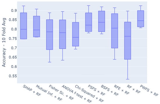
Figure 11.
Comparison of methods.
These results highlight a key point: in domains where data are scarce and expensive to obtain, prioritizing methods that extract the most predictive power, despite longer runtimes, is a rational and justifiable strategy. The additional minutes spent in feature selection or model training are negligible compared to the months or years required to gather the dataset themselves. Researchers should, therefore, view computational time not as a bottleneck but as a necessary investment to ensure model robustness and performance, especially when every percentage gain in accuracy may hold significant practical or scientific value.
It is important to note that the method presented in this paper can be considered the first version of how probabilistic selection is applied to features. There are several directions of future research that can further improve performance or explore the advantages of the method for different applications.
For instance, the learning rate of the weight update equation can be a function rather than a constant that depends on the number of trials, weight variance, and the feature count. This function can become iteratively more aggressive as more individual features have had an opportunity to be trained and tested over the estimator network, or when finer tuning is required at the end of the feature search, the Learning rate value can slowly diminish.
The number of features to be selected does not need to be predefined in the PWFS algorithm; instead, it can be determined adaptively by the algorithm itself. PWFS is capable of monitoring the variance in feature weights during the selection process, and when this variance diminishes, signaling that additional features provide marginal or comparable contributions, it can trigger an early stopping criterion. This mechanism allows the algorithm to suggest an appropriate number of features dynamically, based on the observed importance distribution, rather than relying on a manually specified parameter. Additionally, this approach can help reduce computational expenses by minimizing the number of unnecessary selection trials.
In addition to the linear and golden ratio methods, the slotting algorithm can be further modified to become a function dependent on the performance and current weights of individual features. This can create a trade-off mechanism between the speed and the quality of feature selection and reduce the number of trials necessary when there is a significantly important feature in the mix.
The model can be used to support ensemble learning methods. Ensemble methods use multiple learning algorithms to obtain better predictive performance than that could be obtained from a single algorithm alone. Using this approach, ensemble learning takes care of the overfitting and high variance problems. Multiple models also help remove the bias that could occur from one model.
We can train the models, where a set of the best features and a secondary set of subsidiary features with little replication can be provided to train and test two (or more) algorithms, as visualized in Figure 12, where one can model a different latent space in the data better than in another and vice versa. then, we can access the hidden temporal information.
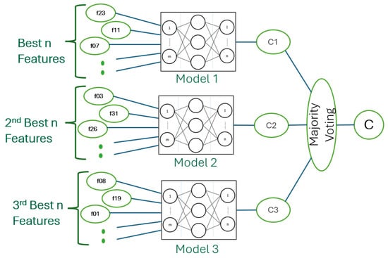
Figure 12.
Using ensemble learning to train and test multiple sets of features and models.
This method allows us to apply ensemble learning in two novel ways: because PWFS is probability-based, every time the algorithm is run, we may end up with a different set of features that result in similar performance metrics. We can use these different sets of features to train ensemble classifiers that can independently perform from one another. Secondly, PWFS allows us to rank features according to their importance. We can train ensemble classifiers with the first, second, and third set of features to access hidden information, capturing other parts of the data that could not be achieved with the usage of only the best set of features.
Author Contributions
Conceptualization, I.U.; methodology, I.U. and M.B.A.; software, M.B.A.; validation, I.U. and M.B.A.; formal analysis, M.B.A.; data curation, M.B.A.; writing—original draft preparation, M.B.A.; writing—review and editing, I.U.; visualization, M.B.A.; supervision, I.U. All authors have read and agreed to the published version of the manuscript.
Funding
This material is based upon work supported by the National Science Foundation under Grant No. 2022299.
Data Availability Statement
The data resources supporting the results can be found on the UCI data repository site. Links to these publicly archived datasets are provided in the references section.
Conflicts of Interest
The authors declare no conflicts of interest.
Abbreviations
The following abbreviations are used in this manuscript:
| ML | Machine Learning |
| PWFS | Probability-Weighted Feature Selection |
| SFS | Sequential Feature Selection |
| RF | Random Forest |
| RFE | Recurrent Feature Elimination |
| ANOVA | Analysis of Variance |
| SHAP | Shapley Additive Explanations |
| MI | Mutual Information |
| ACC | Accuracy |
| CV | Cross-validation |
References
- Li, J.; Cheng, K.; Wang, S.; Morstatter, F.; Trevino, R.P.; Tang, J.; Liu, H. Feature Selection: A Data Perspective. ACM Comput. Surv. 2017, 50, 1–45. [Google Scholar] [CrossRef]
- Gao, W.; Kannan, S.; Oh, S.; Viswanath, P. Estimating Mutual Information for Discrete-Continuous Mixtures. arXiv 2018, arXiv:1709.06212. [Google Scholar]
- Zhou, H.; Wang, X.; Zhu, R. Feature selection based on mutual information with correlation coefficient. Appl. Intell. 2022, 52, 5457–5474. [Google Scholar] [CrossRef]
- Effrosynidis, D.; Arampatzis, A. An evaluation of feature selection methods for environmental data. Ecol. Inform. 2021, 61, 101224. [Google Scholar] [CrossRef]
- Sun, L.; Zhang, X.Y.; Qian, Y.; Xu, J.C.; Zhang, S.G.; Tian, Y. Joint neighborhood entropy-based gene selection method with fisher score for tumor classification. Appl. Intell. 2019, 49, 1245–1259. [Google Scholar] [CrossRef]
- Sun, L.; Wang, T.; Ding, W.; Xu, J.; Lin, Y. Feature selection using Fisher score and multilabel neighborhood rough sets for multilabel classification. Inf. Sci. 2021, 578, 887–912. [Google Scholar] [CrossRef]
- Shakeela, S.; Shankar, N.; Reddy, P.; Tulasi, T.; Koneru, M. Optimal Ensemble Learning Based on Distinctive Feature Selection by Univariate ANOVA-F Statistics for IDS. Int. J. Electron. Telecommun. 2020, 67, 267–275. [Google Scholar] [CrossRef]
- Jamil, M.A.; Khanam, S. Influence of one-way ANOVA and Kruskal–Wallis based feature ranking on the performance of ML classifiers for bearing fault diagnosis. J. Vib. Eng. Technol. 2024, 12, 3101–3132. [Google Scholar] [CrossRef]
- Aggrawal, R.; Pal, S. Sequential Feature Selection and Machine Learning Algorithm-Based Patient’s Death Events Prediction and Diagnosis in Heart Disease. SN Comput. Sci. 2020, 1, 344. [Google Scholar] [CrossRef]
- Guyon, I.; Weston, J.; Barnhill, S.; Vapnik, V. Gene Selection for Cancer Classification Using Support Vector Machines. Mach. Learn. 2002, 46, 389–422. [Google Scholar] [CrossRef]
- Sharma, A.; Singh, M. Batch reinforcement learning approach using recursive feature elimination for network intrusion detection. Eng. Appl. Artif. Intell. 2024, 136, 109013. [Google Scholar] [CrossRef]
- Liu, H.; Zhou, M.; Liu, Q. An embedded feature selection method for imbalanced data classification. IEEE/CAA J. Autom. Sin. 2019, 6, 1–13. [Google Scholar] [CrossRef]
- Zhou, H.; Xin, Y.; Li, S. A diabetes prediction model based on Boruta feature selection and ensemble learning. BMC Bioinform. 2023, 24, 224. [Google Scholar] [CrossRef] [PubMed]
- Sun, Y.; Cao, Y.; Li, P.; Su, S. Sound Based Degradation Status Recognition for Railway Point Machines Based on Soft-Threshold Wavelet Denoising, WPD, and ReliefF. IEEE Trans. Instrum. Meas. 2024, 73, 1–9. [Google Scholar] [CrossRef]
- Sun, Y.; Cao, Y.; Li, P.; Xie, G.; Wen, T.; Su, S. Vibration-Based Fault Diagnosis for Railway Point Machines Using VMD and Multiscale Fluctuation-Based Dispersion Entropy. Chin. J. Electron. 2024, 33, 803–813. [Google Scholar] [CrossRef]
- Hatipoğlu, A.; Süpürtülü, M.; Yılmaz, E. Enhanced Fault Classification in Bearings: A Multi-Domain Feature Extraction Approach with LSTM-Attention and LASSO. Arab. J. Sci. Eng. 2024. [Google Scholar] [CrossRef]
- Marcilio, W.E.; Eler, D.M. From explanations to feature selection: Assessing SHAP values as feature selection mechanism. In Proceedings of the 2020 33rd SIBGRAPI Conference on Graphics, Patterns and Images (SIBGRAPI), Los Alamitos, CA, USA, 7–10 November 2020; pp. 340–347. [Google Scholar] [CrossRef]
- Lee, Y.G.; Oh, J.Y.; Kim, D.; Kim, G. SHAP Value-Based Feature Importance Analysis for Short-Term Load Forecasting. J. Electr. Eng. Technol. 2022, 18, 579–588. [Google Scholar] [CrossRef]
- Er, M.B. Turkish Music Emotion. UCI Machine Learning Repository, 2023. Available online: https://archive.ics.uci.edu/dataset/862/turkish+music+emotion (accessed on 27 May 2025).
- Mansouri, K.; Ringsted, T.; Ballabio, D.; Todeschini, R.; Consonni, V. QSAR Biodegradation. UCI Machine Learning Repository, 2013. Available online: https://archive.ics.uci.edu/dataset/254/qsar+biodegradation (accessed on 27 May 2025).
- Hopkins, M.; Reeber, E.; Forman, G.; Suermondt, J. Spambase. UCI Machine Learning Repository, 1999. Available online: https://archive.ics.uci.edu/dataset/94/spambase (accessed on 27 May 2025).
- Buscema, M.; Terzi, S.; Tastle, W. Steel Plates Faults. UCI Machine Learning Repository, 2010. Available online: https://archive.ics.uci.edu/dataset/198/steel+plates+faults (accessed on 27 May 2025).
Disclaimer/Publisher’s Note: The statements, opinions and data contained in all publications are solely those of the individual author(s) and contributor(s) and not of MDPI and/or the editor(s). MDPI and/or the editor(s) disclaim responsibility for any injury to people or property resulting from any ideas, methods, instructions or products referred to in the content. |
© 2025 by the authors. Licensee MDPI, Basel, Switzerland. This article is an open access article distributed under the terms and conditions of the Creative Commons Attribution (CC BY) license (https://creativecommons.org/licenses/by/4.0/).