Anchor-Free SNR-Aware Signal Detector for Wideband Signal Detection Framework

Abstract

The spectrogram-based wideband signal detection framework has garnered increasing attention in various wireless communication applications. However, the front-end spectrograms in existing methods suffer from visual and informational deficiencies. This paper proposes a novel multichannel enhanced spectrogram (MCE spectrogram) to address these issues. The MCE spectrogram leverages additional channels for both visual and informational enhancement, highlighting signal regions and features while integrating richer recognition information across channels, thereby significantly improving feature extraction efficiency. Moreover, the back-end networks in existing methods are typically transferred from original object detection networks. Wideband signal detection, however, exhibits task-specific characteristics, such as the inherent signal-to-noise ratio (SNR) attribute of the spectrogram and the large variations in shapes of signal bounding boxes. These characteristics lead to issues like inefficient task adaptation and anchor mismatch, resulting in suboptimal performance. To tackle these challenges, we propose an SNR-aware detection network that employs an anchor-free paradigm instead of anchors for signal detection. Additionally, to address the impact of the SNR attribute, we design a trainable gating module for efficient feature fusion and introduce an auxiliary task branch to enable the network to capture more discriminative feature representations under varying SNRs. Experimental results demonstrate the superiority of the MCE spectrogram compared to those utilized in existing methods and the state-of-the-art performance of our SNR-aware Net among comparable detection networks.

1. Introduction

Regulatory agencies, equipment manufacturers, and operators have recently been committed to advancing shared spectrum technologies in the 3.5 GHz and 5 GHz unlicensed bands such as the Citizens Broadband Radio Service (CBRS) and 5G New Radio-Unlicensed (5G NR-U) to further develop their commercial potential [1]. However, the increasingly dense access of wireless devices has led to severe spectrum congestion, necessitating dynamic coexistence among the devices through spectrum monitoring. For example, the CBRS band being opened offers significant opportunities for 5G and IoT applications, provided that radar signals are effectively sensed and protected from interference [2]. Consequently, signal detection and classification, which play a fundamental role in spectrum monitoring, have become increasingly important.

Traditional approaches to signal detection and classification are typically conducted in two separate steps [3]. First, most signal detection methods focus solely on signal presence and exhibit drawbacks such as strict requirements for prior information and high computational complexity [4]. Second, most signal classification methods are designed for narrowband classification, assuming that the classification is performed in independent narrowband transmissions [5]. However, in complex shared-spectrum scenarios, signals must dynamically coexist while dealing with mutual interference and overlap. In these conditions, narrowband classification methods encounter significant performance degradation [6]. Moreover, traditional two-step approaches struggle to characterize parameters such as bandwidth and dwell time for multiple signals. These limitations pose increasing challenges for wireless applications to benefit from traditional methods.

Recently, a spectrogram-based framework for signal detection, classification, and time–frequency localization has attracted widespread attention. It comprises two components: the front-end spectrogram converted from time series and the back-end object detection network [7] from computer vision. The framework is termed wideband signal detection, drawing an analogy to the terminology of object detection. Here, “wideband” highlights its applicability to a wideband receiver scenario, where multiple signals may be randomly distributed across the sample bandwidth with varying time spans. With the dimensional advantage of spectrograms and the multi-task property of object detection, this approach not only enables joint detection and classification of multiple signals but also facilitates their localization in the time–frequency domain [8]. This signifies that the framework can provide more comprehensive time–frequency contextual information, which cognitively empowers the transceiver to make intelligent decisions. These distinct advantages have made it highly popular in various applications, such as wideband modulation classification [5,9,10], spectrum sensing [2,6,8,11,12], RF-based drone detection [3], frequency-hopping signal detection [13], and RF interference (RFI) detection [14].

The initial exploration into the wideband signal detection framework can be traced back to O’Shea et al.’s work [15], where a simple detection network was employed for detecting and localizing radio signals. Subsequent studies have centered on the transfer attempts of various networks at the backend of the framework. Faster R-CNN [16] was first utilized in [8,11] to identify and locate Wi-Fi signals, demonstrating clear advantages over morphological processing methods. However, as a two-stage detection network, Faster R-CNN suffers from slower inference speeds. To address this limitation, a one-stage detection network, single-shot multibox detector (SSD) [17], has been explored in [9,14]. In [9], SSD was trained for modulation classification of multiple signals, achieving significantly improved processing speed but relatively poorer performance compared to Faster R-CNN. Another popular one-stage network, the You Only Look Once (YOLO) series [18], has also been widely investigated due to its excellent balance between performance and speed. Among these, YOLOv3 [19] has garnered particular attention [2,5,10,12]. In [5], YOLOv3 was utilized for joint detection and modulation classification on 10 modulation schemes, exhibiting performance comparable to Faster R-CNN at higher SNR levels but underperforming at lower SNR levels. Beyond YOLOv3, other YOLO variants have also been investigated [3,6,13].

Despite the progress made in the above studies, the current framework is often non-task-oriented, primarily focusing on intuitively applying object detection networks to spectrograms. To further enhance the framework’s performance, we are facing two key challenges as follows.

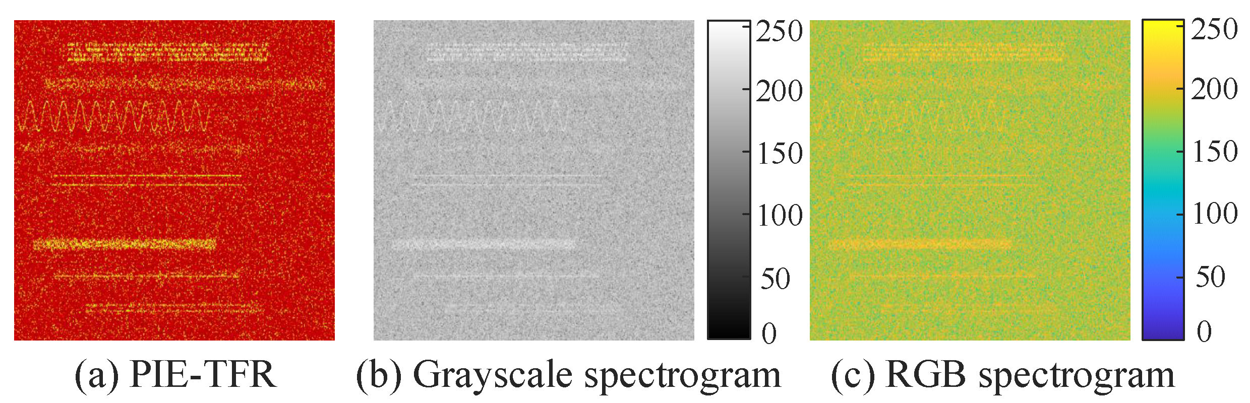
• Front-end spectrograms are underexplored and visually/informationally limited. Specifically, existing studies have only considered two types of spectrograms: grayscale spectrograms obtained through short-time Fourier transform (STFT) and RGB spectrograms derived by applying pseudo-color processing to the grayscale spectrograms. Visually, as the SNR decreases, the contrast between foreground signals and background noise rapidly diminishes in these spectrograms, resulting in indistinct signal regions and time–frequency characteristics. Moreover, they provide limited information gain for recognition and are prone to information degradation. Since spectrograms serve as the data input, these deficiencies can hinder the quality of feature representations extracted by back-end networks.
• Back-end networks lack task-specific customization. Specifically, the aforementioned networks are designed for generic object detection datasets [20], which differ significantly in data manifold characteristics from spectrogram datasets. For example, most existing methods are transferred from the anchor-based networks. However, the signal bounding boxes in spectrograms exhibit more diverse sizes and aspect ratios due to the variability in signal transmission parameters, which makes these anchor-parameter-sensitive networks [21] easily encounter anchor mismatch and performance degradation. Additionally, unique task attributes, such as the SNR, can lead to potential feature impairment and misalignment. The domain-specific prior knowledge related to these attributes has not been effectively incorporated into network design, resulting in limited performance improvements.

To address the aforementioned problems, we propose an enhanced wideband signal detection framework that introduces improvements to both the front-end spectrogram and the back-end network. The main contributions of this paper are summarized as follows.

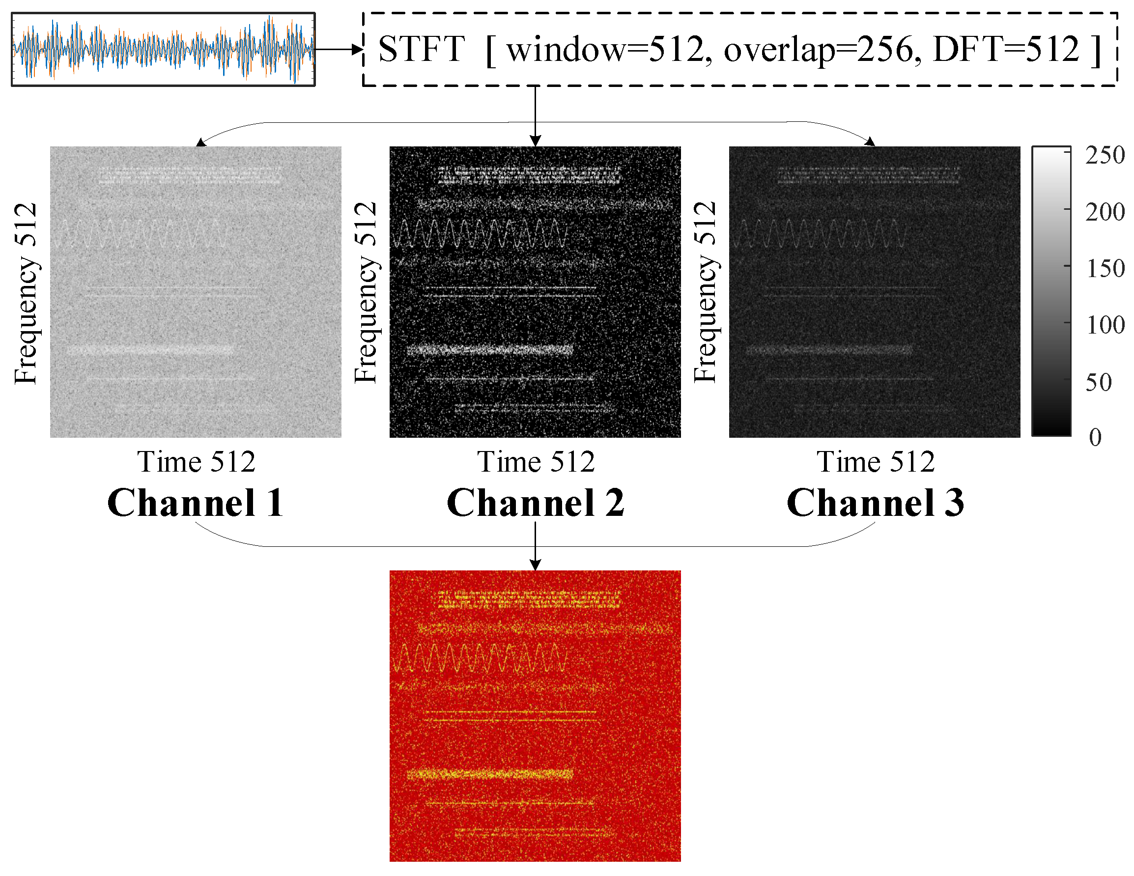
• At the frontend of the framework, a novel multichannel enhanced spectrogram (MCE spectrogram) is proposed. First, a visual enhancement channel is added alongside the base channel to establish a prior attention mechanism. This enables the back-end network to focus more effectively on foreground signals and capture salient visual features. Additionally, an information complementary channel is introduced to explicitly encode extra recognition information within the signal region, thereby improving the semantic feature learning capability of the network.
• At the backend of the framework, we propose a novel SNR-aware network (SNR-aware Net) based on a critical distinction between wideband signal detection and object detection, namely SNR. Firstly, a trainable time–frequency feature gating aggregation module (TFFGAM) is integrated into the neck network, facilitating more task-oriented feature fusion. Furthermore, a multi-task detection head is introduced, which employs the anchor-free paradigm for better generalization to signals with varying bandwidths and durations. In addition to performing classification and regression tasks, the head adds an auxiliary task branch to incorporate the prior knowledge that signals exhibit differentiated characteristics at varying SNRs. This branch enables SNR awareness, effectively alleviating training ambiguities caused by feature misalignment and preventing the network from fitting to weakly discriminative feature representations.
• To evaluate the performance of the MCE spectrogram, we integrate it into several state-of-the-art detection networks designed for wideband signal detection and compare these networks with their counterparts based on traditional spectrogram baselines. We also compare these networks with the proposed SNR-aware Net. Experimental results demonstrate the modality superiority of the MCE spectrogram and the state-of-the-art performance of SNR-aware Net. Additionally, we conduct complexity comparisons and ablation experiments to further analyze the effectiveness of the MCE spectrogram and SNR-aware Net.

The rest of this paper is structured as follows. Section 2 reviews the existing research on the wideband signal detection framework. Section 3 explains the motivations for modifying the front-end spectrogram and back-end network. Details of the MCE spectrogram and SNR-aware Net are provided in Section 4. Performance analysis is presented in Section 5, followed by concluding remarks in Section 6.

2. Related Work

Recent studies have increasingly combined spectrograms and other time–frequency representations (TFRs) with computer vision methods, offering new approaches to signal processing challenges. In this section, we first compare two prominent research areas—signal classification and the wideband signal detection framework—highlighting the technical advantages of the latter. Then, the existing research on wideband signal detection framework is reviewed according to two aspects.

2.1. From Narrowband Signal Classification Towards Wideband Signal Detection Framework

The need for better signal classification performance has driven the combination of TFRs with various powerful image classification models. TFR-based signal classification can be divided into modulation classification [22,23,24] and radio access technology classification [1,25,26], both extensively investigated. However, these studies focus on narrowband signal classification, where the TFR utilized as a training sample cannot be directly derived from the compound signals to establish a one-to-one correspondence with the category label. Traditional two-step methods for signal detection and classification have relied on techniques such as refined channelization designs [27] or blind signal separation [28] to satisfy the narrowband classification assumption. Nevertheless, meeting this constraint becomes increasingly difficult in the noisy spectrum, resulting in performance degradation. To address the challenges of wideband classification for compound signals, two new approaches have been attempted. The first approach involves traversing all possible signal combinations and assigning them mutually exclusive class labels [1]. However, this method becomes computationally infeasible as the number of signal classes grows. An alternative approach inspired by multi-label image classification has also been explored [29], where compound signals are assigned a label vector containing the semantic meanings of all mixed components [30]. Despite its potential, this method faces challenges such as class imbalance and complex labeling requirements. Additionally, critical parameters like signal bandwidth and duration cannot be derived from a sole classification task.

The growing need for wideband signal processing, coupled with the benefits of time–frequency localization, has led to increased attention on another computer vision task, object detection. Object detection involves detecting, classifying, and locating all instances within an image using a multi-output architecture. When applied to TFRs, this approach gives rise to the wideband signal detection framework [15].

2.2. Wideband Signal Detection Framework

2.2.1. Front-End Spectrogram

Although various time–frequency transformations, such as the smooth pseudo Wigner–Ville distribution [22,24] and S-transform [23,25], have been applied in signal classification, studies on the wideband signal detection framework have predominantly favored and all chosen STFT-based spectrograms. This preference is attributed to the simplicity of implementation, computational efficiency, and absence of cross-term interference in multi-signal scenarios that STFT offers. Existing spectrograms can be categorized into two types based on their visual modality: grayscale spectrograms, as utilized in [6,8,9,10,11,13], and pseudo-color RGB spectrograms, as employed in [3,5,12]. Furthermore, variations in the selection of STFT parameters result in differences in spectrogram size and resolution. For instance, [11] utilized a window length and overlap of 5600 and 2800 points, respectively, while [13] adopted a shorter 256-point window with a larger 91% overlap.

Despite these efforts, limited attention has been devoted to addressing the visual and informational limitations of existing spectrograms. This gap highlights the need for further research into enhancing the quality and effectiveness of spectrograms in the wideband signal detection framework.

2.2.2. Back-End Detection Network

As discussed earlier, previous studies have investigated various object detection networks. In these attempts, the networks have undergone certain modifications that primarily focus on two aspects. The first aspect involves utilizing the Intersection over Union (IoU)-series localization loss functions [31] for more precise regression. For instance, Generalized IoU (GIoU) loss [32] was used in [5,13], while Complete IoU (CIoU) loss [33] was adopted in [10,12]. Additionally, Distance IoU (DIoU) [33] was utilized during inference in [10] to improve the accuracy of non-maximum suppression. Secondly, efforts have been made to reduce the network size for greater efficiency. Considering the relatively simpler nature of signal detection in spectrograms compared to object detection in natural images, downscaled variants were employed in [8,15]. Furthermore, to enhance inference speed, Refs. [12,13] replaced the original backbone networks with lightweight architectures such as GhostNet [34] and MobileNet [35], respectively.

Despite these modifications, most approaches have directly borrowed techniques from object detection without accounting for the fundamental differences between wideband signal detection and object detection tasks. As a result, these adaptations may lead to limited performance improvements or even no effect at all. A critical distinction lies in the consideration of SNR, which has been largely overlooked in prior studies. Unlike object detection, where targets in natural images are not typically associated with varying SNRs, spectrograms derived from time series inherently possess an SNR attribute. Therefore, analyzing the impact of SNR on aspects such as feature extraction and network training is essential for developing more targeted and effective network components tailored to wideband signal detection.

3. Motivation

3.1. Towards a More Spectrogram-Centric Framework

Previous works have tended to be network-centric, focusing on the attempts of various back-end detection networks [4,5]. However, this approach has certain limitations. First, these networks are designed for specific object detection datasets, leading to a decline in performance when directly applied to spectrograms. Moreover, it involves complex parameter tuning and layer configurations [8], impacting deployment efficiency.

In contrast, we prioritize a spectrogram-centric framework, which offers more consistent and rewarding outcomes. Given their data-driven nature, various network models inherently reflect the trained data, making high-quality data crucial for ensuring predictable performance [7]. Further, unlike natural images, spectrograms are derived from a transformation process before being used as an input modality. This transformation step provides an opportunity to enhance the spectrogram itself, thereby increasing signal separability and improving the training efficiency and performance of the back-end network.

3.2. Towards a More Tailored SNR-Specific Framework

Previous studies have actually approached the framework from a visual perspective, aiming to optimize performance by transferring well-established object detection networks [4,15]. While this approach has yielded some success, task-specific networks with superior performance often require reliance on prior domain knowledge. Our motivation lies in treating the framework as both a visual task and a domain-specific task. To this end, our modifications leverage both insights from object detection and the distinctions between wideband signal detection and object detection, enabling the customization of more prior-knowledge-guided network components. We specifically focus on the key difference, SNR, and analyze its impacts on the network as follows.

(1) Impaired Feature Representations Due to the SNR Attribute. In natural images, foreground objects and backgrounds are clearly separated, allowing networks to extract features from their respective regions. However, due to the inherent SNR attribute, foreground signals in spectrograms are always noise overlap-added, resulting in inevitably impaired feature extraction from signal regions [8]. While feature fusion offers a potential solution to this issue, the feature fusion components in object detection networks are designed based on the characteristics of generic objects and are not well suited to recalibrating the impaired features encountered in wideband signal detection. Therefore, it is necessary to design a more targeted feature fusion mechanism to obtain more robust feature representations.

(2) Feature Misalignment Due to Varying SNRs. Due to varying degrees of noise influence, even signals of the same class exhibit differentiated time–frequency characteristics at different SNRs. This differentiation differs from the concept of intra-class diversity, but rather a result of the random impairment of signal features by noise. However, relying solely on the gradients of the classification loss forces the network to fit the signals with the same class but varying SNRs, thereby suffering from the misalignment of the differentiated and impaired features. It introduces training ambiguity and causes the network to collapse into non-critical feature representations. This is distinct from object detection, and putting the solution to such SNR-specific challenges into the object detection pipelines will not be effective. In contrast, when humans identify signals in spectrograms, prior knowledge about the differentiated features at varying SNRs is naturally utilized. Typically, this involves first assessing the SNR range and then recognizing signals based on the specific features exhibited at particular SNRs. Motivated by this observation, our goal is to incorporate this prior knowledge into the network design, enabling the network to become SNR-aware. By doing so, the network can effectively capture more discriminative features along both the signal class and SNR dimensions during training, thereby alleviating the feature misalignment.

4. Methodology

The improved framework is described in detail in this section, comprising the front-end MCE spectrogram and the back-end anchor-free SNR-aware Net. The pipeline is illustrated in Figure 1, where SNR-aware Net is decoupled into three components: the backbone network, the neck network, and the detection head.

4.1. MCE Spectrogram

Let $\mathit{x}\left(k\right)$ be the sampled time series. The discrete Fourier transform is computed and then added to the complex-valued matrix $\mathit{S}(n,m)$ to obtain the STFT of $x\left(k\right)$:

$$\mathit{S}(n,m)=\sum _{k=0}^{N-1}{e}^{-j2\pi {\displaystyle \frac{kn}{N}}}\mathit{w}\left(k\right)\mathit{x}(k+m(N-O)),$$

(1)

where $\mathit{w}$ is an analysis window of length N. The window slides over $\mathit{x}\left(k\right)$ at an overlap of O samples between adjoining segments. n and m are the frequency bin (row) index and time bin (column) index of $\mathit{S}$, respectively.

The spectrogram is defined as the squared magnitude of $\mathit{S}$, given by $\mathit{P}={\mathit{SS}}^{*}$. Previous studies utilize the log-transformed spectrogram and the RGB spectrogram as input. However, considering the characteristics of the spectrogram and network, it is necessary to reexamine these spectrograms from both visual and informational perspectives:

Firstly, spectrograms are fed into the network as an image-like modality. A central theme of processing vision tasks with the network is to capture the most salient visual features for a given task from foreground targets. However, as the SNR decreases, foreground signals in these spectrograms are quickly overwhelmed by background noise, resulting in unclear signal features such as textures.

Secondly, the information encoded in the variations between time–frequency bins is what signal recognition inherently needs. Correspondingly, the network naively learns crucial semantic features through end-to-end training by activating informative regions. However, these spectrograms provide only limited information gains. Specifically, the grayscale spectrogram, being a single-channel matrix, is highly susceptible to interference. The RGB spectrogram is a pseudo-color representation, which does not provide additional information but may introduce mapping errors.

To address the limitations of the above spectrograms, we propose the MCE spectrogram by leveraging channels for both visual and informational enhancement, as illustrated in Figure 2. The details of each channel are outlined below.

4.1.1. Channel 1 (Base Channel)

The log-transformation enables better control over the dynamic range of the spectrogram matrix, facilitating the emphasis on variation details with low grayscale intensity. As a result, the log-transformed spectrogram matrix is assigned to the first channel, which serves as a base channel of the overall MCE spectrogram. It provides a visually comprehensive view of foreground signals and background noise while preserving sufficient time–frequency contextual information.

Furthermore, the base channel is utilized to anchor the size of the MCE spectrogram to $512\times 512$. This input size not only effectively satisfies the performance–speed trade-off but also ensures the equilibrium of the receptive field along the time and frequency directions during subsequent convolution operations. Additionally, this size aligns with common practices in computer vision tasks, making it easier to reference complex network layer configurations and avoiding information loss from resizing operations.

After obtaining the spectrogram matrix $\mathit{P}$, we further log-transform and normalize it to [0, 255] using the following:

$${\mathit{P}}_{\log }=10lo{g}_{10}\mathit{P},{\mathit{P}}_{c1}={\displaystyle \frac{{\mathit{P}}_{\log }-min\left({\mathit{P}}_{\log }\right)}{max\left({\mathit{P}}_{\log }\right)-min\left({\mathit{P}}_{\log }\right)}}\times 255,$$

(2)

where the matrix ${\mathit{P}}_{c1}$ is ultimately placed in the first channel.

4.1.2. Channel 2 (Visual Enhancement Channel)

A visual enhancement channel is then introduced to emphasize foreground signals over background noise, thereby effectively improving the visual feature extraction efficiency of the back-end network. Specifically, we propose a novel statistical thresholding method based on histogram statistics of the spectrogram to filter out pixels in the noise region and retain those in the signal region without relying on SNR information.

As shown in Figure 3, the histogram statistical characteristics of ${\mathit{P}}_{c1}$, derived from the mixed signal in Figure 2, vary at different SNR levels. Here, SNR is defined as the ratio of the mixed signal, which contains multiple signal components, to the background noise. At higher SNRs, the intensity values of the signal and noise regions are clearly distinguishable, resulting in a bimodal histogram distribution. As the SNR decreases, these distributions gradually overlap, leading to reduced contrast and less distinct signal areas. Notably, it can be also observed that the statistical distribution of the noise presents similarity. Specifically, $t_{75}$ in Figure 3 represents an intensity value where pixels with values lower than $t_{75}$ account for 75% of the total pixel count (i.e., $512\times 512\times 0.75$). Although the four specific $t_{75}$ values differ across SNRs, they are positioned similarly in the distribution. Thus, a statistical threshold can be effectively set to filter out a consistent percentage of noise while preserving foreground signals, even across varying SNRs.

The threshold ${\mathit{P}}_{c1}$ is then assigned to the second channel, which establishes a prior, equivalent attention mechanism, enabling the back-end network to better focus on and capture features of the signal regions. As shown in Figure 2, the contrast between the foreground signals and background noise of ${\mathit{P}}_{c2}$ is markedly improved. Moreover, the signal regions are distinctly highlighted after channel concatenation.

4.1.3. Channel 3 (Information Complementary Channel)

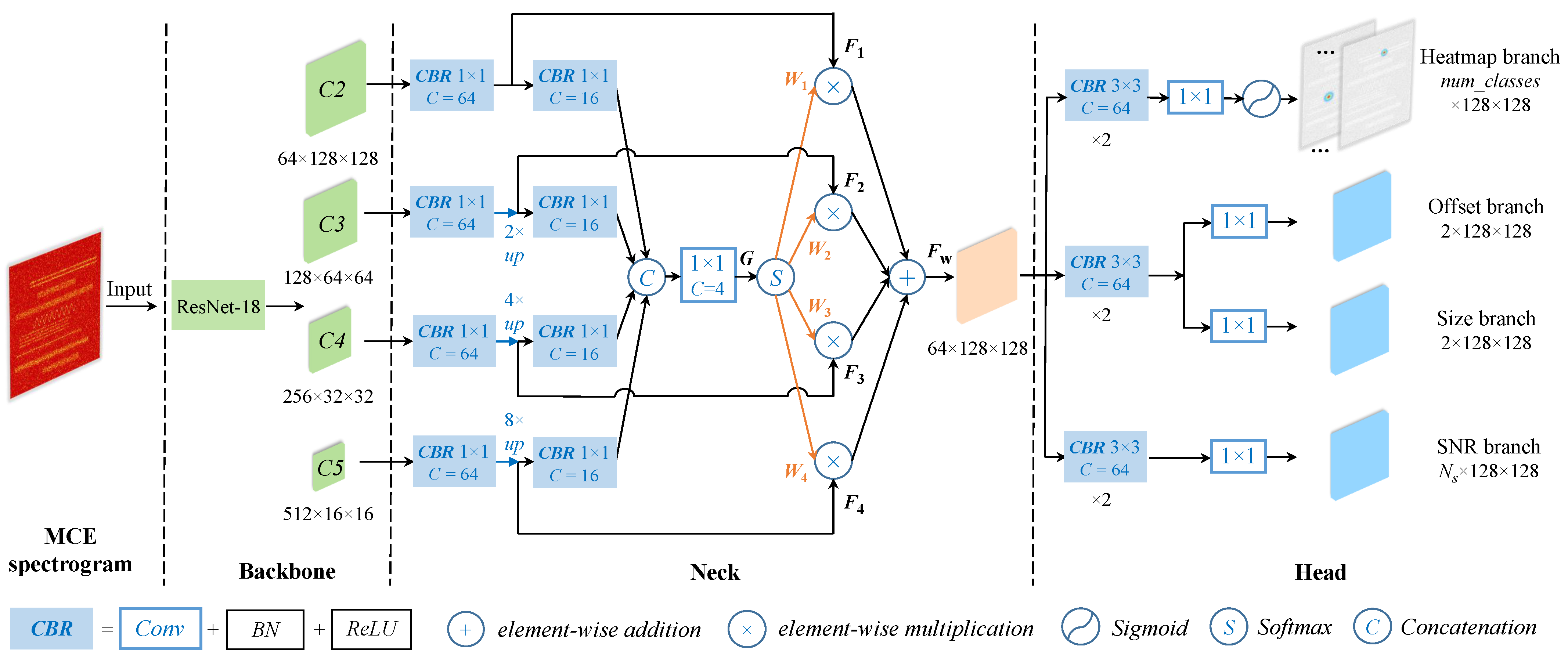
In addition to the intuitive visual feature impairment, implicit information degradation also significantly impacts the performance. To address this issue, we introduce a information complementary channel to perform the informational enhancement. It explicitly incorporates more recognition information across the channels, thereby improving the semantic feature extraction efficiency of the back-end network.

We naturally introduce $\mathit{P}$ due to the following considerations: (1) While ${\mathit{P}}_{c1}$ enhances details in low-grayscale-intensity areas, it compresses and impairs high-intensity regions. The matrix $\mathit{P}$ serves as a complementary component, explicitly introducing additional recognition information into the spectrogram. (2) Compared to ${\mathit{P}}_{c1}$, $\mathit{P}$ undergoes an equivalent antilogarithm transformation, visually emphasizing high-intensity areas. As a result, important signal features such as outlines and textures are further highlighted, as depicted in Figure 2. (3) Since $\mathit{P}$ is an intermediate matrix in the generation of ${\mathit{P}}_{c1}$, it can be derived without additional computational complexity. After using the same normalization in Equation (2), the matrix $\mathit{P}$ is assigned to the third channel.

Figure 4 depicts a visual comparison of the MCE spectrogram, grayscale spectrogram, and RGB spectrogram (using the same colormap as in [3,5,12]) at -5dB SNR. By contrast, the MCE spectrogram, obtained by concatenating three channels, is a true-color representation without a color bar. It not only highlights signal regions and texture features more distinctly but also integrates more signal recognition information across the channels. Moreover, the MCE spectrogram is concise, as its three channels can be obtained through a single STFT operation.

4.2. SNR-Aware Net

As illustrated in Figure 1, SNR-aware Net comprises three components: (1) the backbone, responsible for feature extraction; (2) the neck, incorporating a TFFGAM for feature fusion and recalibration; and (3) the detection head, consisting of four branches to perform signal classification, time–frequency coordinate regression, and SNR awareness.

4.2.1. Backbone

Wideband signal detection within the MCE spectrogram involves lower task complexity than object detection in natural images, obviating the need for a backbone network with excessive model complexity. As a result, we have adopted ResNet-18 [36] as our backbone among various models. As depicted in Figure 1, the backbone generates four different levels of feature maps, $\mathit{C}2$-$\mathit{C}5$, each with varying channels and down-sampling ratios.

4.2.2. Neck

As mentioned earlier, the SNR attribute is accompanied by impaired feature representations. Nevertheless, different levels of the feature hierarchy contribute differently to signal detection and recognition at different SNRs. At higher SNRs, signal textures are more distinct, making low-level features more effective. As SNR decreases, clear visual features become distorted, and higher-level features become more important due to their stronger semantic content and implicit robustness to noise, which arises from the smoothing effect of multiple convolution operations. Therefore, it is essential to design a targeted neck component to effectively leverage and fuse features from different levels, thereby enhancing the quality of feature representations. However, previous studies have largely overlooked the importance of the neck. Some approaches either omit this component or directly adopt original neck architectures designed based on the characteristics of generic objects such as the Feature Pyramid Network [37], leading to suboptimal fusion effectiveness.

We propose a TFFGAM to achieve more task-oriented feature fusion, as illustrated in Figure 1. Firstly, each of $\mathit{C}2$-$\mathit{C}5$ undergoes a CBR unit with 64 channels. Subsequently, we upscale the resolutions of $\mathit{C}3$-$\mathit{C}5$ to $128\times 128$ using interpolation with different ratios to obtain ${\mathit{F}}_1$-${\mathit{F}}_4$. To simplify network training, we use nearest-neighbor interpolation instead of transpose convolution. After that, ${\mathit{F}}_1$-${\mathit{F}}_4$ are sent to four CBR units to reduce their channel dimension to 16 for memory efficiency. They are then concatenated and passed through a shared $1\times 1$ convolution layer, producing $\mathit{G}\in {\mathbf{R}}^{4\times 128\times 128}$. To ensure that the weights sum to 1, we apply the softmax function to process $\mathit{G}$ along the channel dimension, yielding four gating weight maps {${\mathit{W}}_i\in {\mathbf{R}}^{1\times 128\times 128},i\in \{1,2,3,4\}$}. Finally, these weight maps are broadcasted and used to reweight ${\mathit{F}}_1$-${\mathit{F}}_4$, generating the final refined feature maps ${\mathit{F}}_w\in {\mathbf{R}}^{64\times 128\times 128}$:

$${\mathit{F}}_w=\sum _{i=1}^4{\mathbf{W}}_i·{\mathit{F}}_i,$$

(3)

where [·] denotes element-wise multiplication. During the above process, the parameters of the weight maps are learnable, enabling the network to automatically fuse effective features while suppressing those that are heavily degraded by noise.

4.2.3. Head

Anchor-based heads rely on the pre-defined anchor boxes to match target boxes, which often encounter anchor mismatch issues due to the variability in signal bandwidth and duration. In contrast, anchor-free heads eliminate this problem and offer a more straightforward solution for wideband signal detection. In this study, we employ a keypoint-based anchor-free paradigm. As illustrated in Figure 1, the feature maps from the neck are fed into four task branches. The heatmap branch generates a keypoint heatmap, where the peaks in the heatmaps are used to locate the center points of signals. Signal classification is performed based on the responses across the channel dimension at these peak locations. The offset branch compensates for the regression errors of the center point coordinates, while the size branch predicts the height and width of the target. Additionally, we add an auxiliary task branch for SNR awareness.

(1) Heatmap branch

The heatmap branch finally generates the predicted keypoint heatmaps ${\widehat{\mathit{Y}}}_{c,x,y}\in {[0,1]}^{num\_classes\times 128\times 128}$, where each channel corresponds to a signal class. A prediction ${\widehat{\mathit{Y}}}_{c_1,x_1,y_1}=0.9$ indicates the presence of a signal of category $c_1$ with its center at $(x_1,y_1)$ and a class confidence of 0.9.

The ground truth (GT) heatmaps ${\overline{\mathit{Y}}}_{c,x,y}$ are derived by splatting the GT center points in the original image onto the equivalent low-resolution heatmaps using a 2D Gaussian kernel. For example, assuming the existence of a signal of the category $c_0$ with its center at $\mathit{o}=(o_x,o_y)$ in the original image, the GT heatmaps can be obtained by

$${\overline{\mathit{Y}}}_{c_0,x,y}=exp\left(-{\displaystyle \frac{{(x-{\overline{o}}_x)}^2+{(y-{\overline{o}}_y)}^2}{2{\sigma }^2}}\right),$$

(4)

where $\overline{\mathit{o}}=({\overline{o}}_x,{\overline{o}}_y)=\lfloor {\displaystyle \frac{\mathit{o}}{4}}\rfloor$ represents the equivalent center point, and $\sigma$ is the adaptive standard deviation relative to the size of bounding boxes. In the $c_0$th channel, the GT value at $\overline{\mathit{o}}$ is 1, gradually diminishing to 0 away from the center point. We use the Gaussian focal loss [38] to train the heatmap branch:

$$L_{hp}={\displaystyle \frac{-1}{N}}\sum _{c,x,y}\left\{\begin{array}{cc}{(1-{\widehat{\mathit{Y}}}_{c,x,y})}^{\alpha }\log \left({\widehat{\mathit{Y}}}_{c,x,y}\right)\hfill & \mathrm{if}{\overline{\mathit{Y}}}_{c,x,y}=1\hfill \\ \begin{array}{c}{(1-{\overline{\mathit{Y}}}_{c,x,y})}^{\beta }{\left({\widehat{\mathit{Y}}}_{c,x,y}\right)}^{\alpha }\\ \log (1-{\widehat{\mathit{Y}}}_{c,x,y})\end{array}\hfill & \mathrm{otherwise},\hfill \end{array}\right.$$

(5)

where N is the number of center points, and the hyperparameters $\alpha$ and $\beta$ are set to two and four, respectively.

(2) Offset branch

Equation (4) reveals the rounding errors that occur between the coordinates of center points in the original image and their equivalent integer-valued coordinates in the GT heatmap. The inherent imprecision of the GT center points will lead to imprecise predicted center coordinates. To address this issue, the offset branch is introduced to predict the center offset maps $\widehat{\mathit{O}}\in {\mathbf{R}}^{2\times 128\times 128}$, compensating for each center point during the decoding process. We use the smooth L1 loss to train the regression of the offset branch:

$$L_{off}={\displaystyle \frac{1}{N}}\sum _{i=1}^N{\mathrm{smooth}}_{\mathrm{L}1}\left(\widehat{{\mathit{O}}_i}-\left({\displaystyle \frac{{\mathit{o}}_i}{4}}-\overline{{\mathit{o}}_i}\right)\right),$$

(6)

where N, $\mathit{o}$, and $\overline{\mathit{o}}$ have the same meaning as above, indicating that the offset loss only acts on the center point positions. The smooth L1 loss is described by

$${\mathrm{smooth}}_{\mathrm{L}1}\left(x\right)=\left\{\begin{array}{cc}0.5x^2,\hfill & \mathrm{if}\left|x\right|<1\hfill \\ \left|x\right|-0.5\hfill & \mathrm{otherwise}.\hfill \end{array}\right.$$

(7)

(3) Size branch

After obtaining the categories and center points of the signals, it is then necessary to regress their sizes. Therefore, the size branch is used to predict the size maps $\widehat{\mathit{S}}\in {\mathbf{R}}^{2\times 128\times 128}$, where the two channels correspond to the predicted height and width of the signal box, respectively. We also employ the smooth L1 loss to train the size branch:

$$L_{size}={\displaystyle \frac{1}{N}}\sum _{i=1}^N{\mathrm{smooth}}_{\mathrm{L}1}\left(\widehat{{\mathit{S}}_i}-{\mathit{S}}_i\right),$$

(8)

where $\mathit{S}$ is the GT size.

(4) SNR branch

As previously discussed, the time–frequency characteristics of signals such as the outlines and textures, exhibit significant variations across different SNRs. For a network that is driven solely by the gradients of classification loss, these variations and impairments in features at different SNRs can lead to feature misalignment, negatively impacting both network training and performance. To mitigate this issue, we utilize the prior knowledge that signals exhibit varying characteristics at varying SNRs to modify the network architecture. Specifically, as shown in Figure 1, an SNR branch is introduced to make the network SNR-aware. This branch explicitly establishes a mechanism that enables the network to treat both category and SNR as inherent attributes of the signal during feature learning. By doing so, the network captures more prior-knowledge-guided category differences through an approach similar to attribute recognition. In this process, the classification task-related gradient backpropagation is optimized, reducing training ambiguity caused by feature misalignment and preventing the network from falling into fewer discriminative features.

Specifically, to enhance the efficiency of training convergence, we approach the SNR awareness as a classification problem rather than a regression one by assigning distinct class labels to different SNR ranges. The focal loss [21] is utilized to train the SNR branch:

$$L_{SNR}={\displaystyle \frac{1}{N}}\sum _{i=1}^N{L}_{\mathrm{focal}}\left(\widehat{{\mathit{p}}_i},{\mathit{p}}_i\right),$$

(9)

where ${\mathit{p}}_i$ is the GT SNR labels and $\widehat{{\mathit{p}}_i}$ is the predicted $N_s$D vector. $N_s$ is the number of classified SNR ranges. Following [21], we adopt a strategy of training $N_s$ binary classifiers instead of utilizing a multi-class classifier. For each binary classifier, focal loss can be described as

$$L_{\mathrm{focal}}\left(\widehat{y},y\right)=\left\{\begin{array}{cc}-\mu {(1-\widehat{y})}^{\gamma }log\left(\widehat{y}\right),\hfill & \mathrm{if}y=1\hfill \\ -(1-\mu ){\widehat{y}}^{\gamma }log(1-\widehat{y})\hfill & \mathrm{otherwise},\hfill \end{array}\right.$$

(10)

where $\widehat{y}$ is the predicted probability for the GT class with label $y=1$. The hyperparameters $\mu$ and $\gamma$ are set to 0.25 and 2, respectively.

5. Experiments

5.1. Experimental Settings

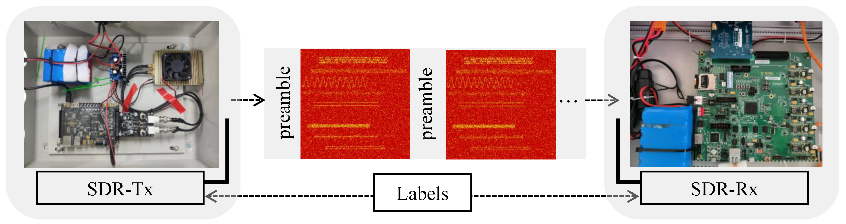
5.1.1. Dataset Generation

Figure 5 illustrates the workflow for creating a labeled dataset, which combines both synthetic signal generation and real-world data capture techniques. Specifically, the labels for the spectrograms are automatically generated by logging the parameters used during the synthetic data generation process. These parameters are detailed in

Table 1. Parameter settings of dataset generation.

Parameters	Range of Values
Number of signals	[5, 8]
Time–frequency span of spectrogram	182.4 ms/720 kHz
Duration of each signal	[45.6 ms, 182.4 ms]
Signal categories	BPSK, QPSK, 2ASK, 16QAM, 2FSK, 4FSK, MSK, FM, AM-DSB
Symbol rate of each signal	[24 kHz, 40 kHz]
${\mathrm{SNR}}_{average}$	[−20 dB, 15 dB]

. The signals are then transmitted and collected over-the-air, introducing real-world impairments. To ensure label consistency between the transmitter and receiver, we implemented a synchronization mechanism that periodically transmits preambles. For signal collection, we used a custom RF transceiver equipped with a vertically polarized omnidirectional antenna.

Evaluating the performance of the proposed method at different SNR levels is necessary. However, with practical signals, it is challenging to precisely control the SNRs. To address this, we adopt the approach from [3] by adding raw signals and additive white Gaussian noise (AWGN) to build datasets with varying average SNRs (${\mathrm{SNR}}_{average}$). Since the power and bandwidth differ for signals in a multi-signal scenario, the actual SNR for each signal can vary slightly [3]. Therefore, the SNR of each signal (${\mathrm{SNR}}_{sig}$) is also calculated to obtain the class labels of the SNR range for training the SNR branch. Specifically, the coordinate labels are first utilized to automatically locate the signal and noise regions in the time–frequency domain. Next, we average the signal and noise areas along the time dimension to obtain their equivalent frequency-domain representations. Following this, the frequency–domain SNR calculation method [3] is applied to estimate the SNR for each signal. This approach can be easily integrated into the labeling process, whether through automatic label generation or manual annotation, and temporal averaging helps reduce estimation errors. A total of 2500 samples are generated at each ${\mathrm{SNR}}_{average}$. We divide the training, validation, and test sets in a 4:2:4 ratio. After calculating the ${\mathrm{SNR}}_{sig}$, we convert it into the class label. The correspondence is as follows: [−20 dB, −16 dB]∼0, [−15 dB, −11 dB]∼1, [−10 dB, −6 dB]∼2, [−5 dB, −1 dB]∼3, [0 dB, 5 dB]∼4, and [6 dB, 15 dB]∼5.

5.1.2. Evaluation Metrics

Considering the multi-task property of the framework, we adopt widely-used metrics from object detection, including average precision (AP), mean AP (mAP), and mean average recall (mAR) [39]. AP measures both the accuracy of signal classification and the precision of time–frequency localization for each category. mAP is the mean of APs across all categories. mAR, similar to the probability of detection, evaluates the detector’s ability to find all signals of interest. These metrics achieve high scores only when the signals are fully detected, accurately classified, and precisely localized. To ensure a rigorous evaluation, these metrics are calculated at all intersection over union (IoU) thresholds.

5.1.3. Implementation Details

To assess the modality superiority of the MCE spectrogram, we combine it with SNR-aware Net and three other state-of-the-art networks used in previous works. We then compare these combinations with counterparts based on the baseline spectrograms (grayscale and RGB). Additionally, we conduct a comprehensive evaluation to verify the superior performance of SNR-aware Net compared to these networks. The details of the networks are as follows:

• Faster R-CNN: For a fair comparison, we adjust Faster R-CNN as suggested in [8], including configuring the backbone as pre-trained VGG-13 and reducing channels.
• SSD: Following [9], the backbone is configured as VGG-16, with default anchor settings and loss functions.
• YOLOv3: Adjustments are made to YOLOv3 following [5], including configuring the backbone as DarkNet-53 and replacing the localization loss function.

We utilize the AdamW optimizer and add 7.2 k warm-up iterations. The learning rate is initialized to 1 × 10⁻³ and decays using a cosine annealing scheduler. The models are trained for 80 epochs with a batch size of 64, distributed on four NVIDIA Tesla K80 GPUs.

5.2. Performance Analysis

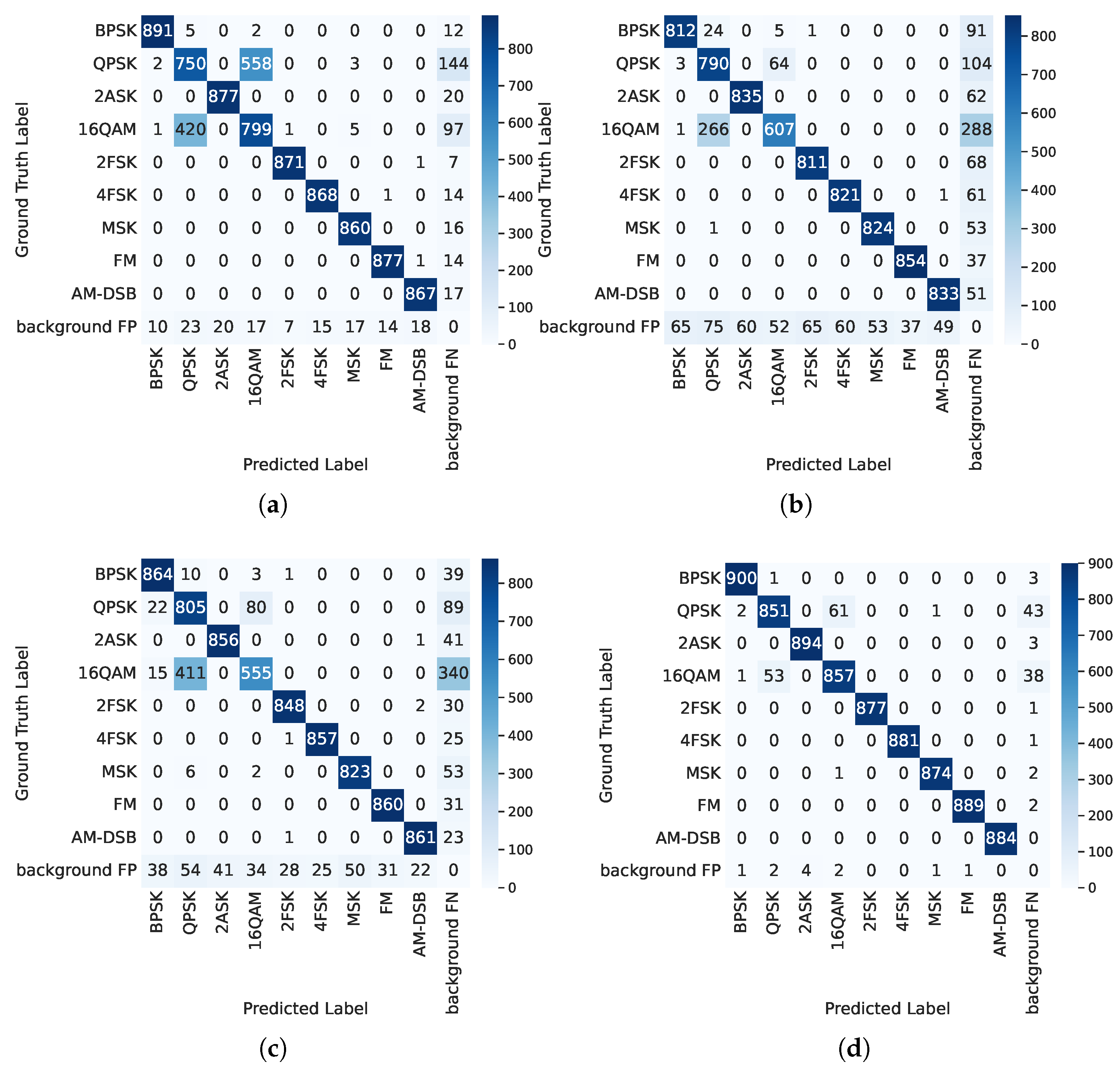
5.2.1. Effectiveness Verification of MCE Spectrogram

The comparison methods are not limited to specific combinations of networks and spectrograms used in previous works. Instead, each network is paired with both grayscale and RGB spectrogram baselines to provide a comprehensive comparison, as detailed in

Table 2. Performance comparisons in terms of AP (%), MAP (%), and MAR (%) between MCE spectrogram and spectrogram baselines in combination with different detection networks.

Spectrogram Modality	Detector	mAP	mAR	BPSK	QPSK	2ASK	16 QAM	2FSK	4FSK	MSK	FM	AM-DSB
Grayscale spectrogram		68.7	84.7	65.3	38.7	75.0	40.2	85.2	78.8	74.9	79.0	81.1
RGB spectrogram	Faster R-CNN [8]	71.0	85.2	63.7	41.7	76.1	51.1	84.6	80.4	75.3	83.2	82.9
MCE spectrogram		77.1	87.5	79.1	49.9	79.7	55.0	89.3	84.4	84.2	86.4	85.9
Grayscale spectrogram		64.3	81.6	62.2	34.3	71.1	33.4	78.8	75.3	71.9	74.9	76.9
RGB spectrogram	SSD [9]	63.1	80.6	62.8	32.4	70.8	35.7	75.3	73.9	72.3	71.3	73.7
MCE spectrogram		70.6	83.0	63.0	52.7	75.5	51.1	82.2	77.4	73.8	81.4	78.6
Grayscale spectrogram		64.5	81.6	64.0	33.9	73.6	36.7	75.6	74.4	73.1	73.4	76.0
RGB spectrogram	YOLOv3 [5]	65.7	82.5	64.4	31.1	73.0	38.9	80.9	76.2	72.5	75.1	78.7
MCE spectrogram		72.9	85.9	66.6	51.8	77.9	47.8	86.6	82.0	76.4	83.7	83.5
Grayscale spectrogram		71.9	84.1	67.4	54.8	75.6	53.9	83.3	78.0	74.1	81.3	79.0
RGB spectrogram	SNR-aware Net	72.8	85.6	64.2	52.1	76.1	55.6	86.9	80.0	78.0	79.8	82.3
MCE spectrogram		80.9	90.7	74.1	64.9	82.2	64.6	92.4	88.3	83.5	89.6	88.8

. The results from the four sets of comparisons clearly show that networks using MCE spectrograms consistently outperform their counterparts based on the spectrogram baselines in terms of mAP and mAR. This superiority can be attributed to the enhanced input data modality provided by the MCE spectrogram, which effectively improves the training efficiency and performance of different back-end networks.

Moreover, the networks based on the MCE spectrogram show improvements across all signal classes in terms of AP scores. As shown in Table 2, signals with distinct texture characteristics, such as FSK and FM, achieve greater AP boosts due to the attention mechanism established by the visual enhancement channel. This mechanism enhances the visual feature extraction efficiency of the networks. Additionally, for visually similar signals such as QPSK and QAM, the information gain from the information complementary channel plays a crucial role. By adding more explicit information along the channels for semantic feature learning during training, the recognition performance is improved.

Furthermore, we investigate the performance comparisons across different SNR levels, as shown in Figure 6. Taking SNR-aware Net as an example, when the SNR exceeds −5 dB, the MCE spectrogram achieves 9.4% and 8.3% higher mAPs compared to grayscale and RGB spectrograms, respectively, along with 5.5% and 4.5% higher mARs. When the SNR is between −20 dB and −5 dB, the mAP of the MCE spectrogram increases by 8.9% and 6.6% over grayscale and RGB spectrograms, while the mAR increases by 8.1% and 6%, respectively. Similarly, although the extent of improvement varies among networks, the MCE spectrogram consistently provides performance gains for the other three networks at both high and low SNRs, further demonstrating its modality superiority. This outcome is expected because the visual enhancement channel enables the network to focus more effectively on signal regions for feature extraction even at low SNRs. Additionally, the information complementary channel provides additional information support at higher SNRs and helps the recognition information encoded in signal regions less affected by noise as SNR decreases.

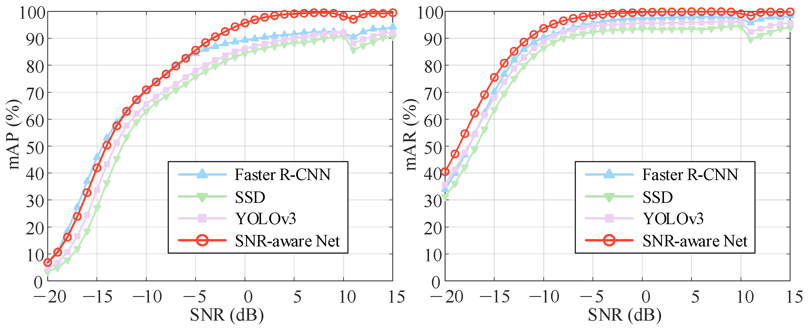
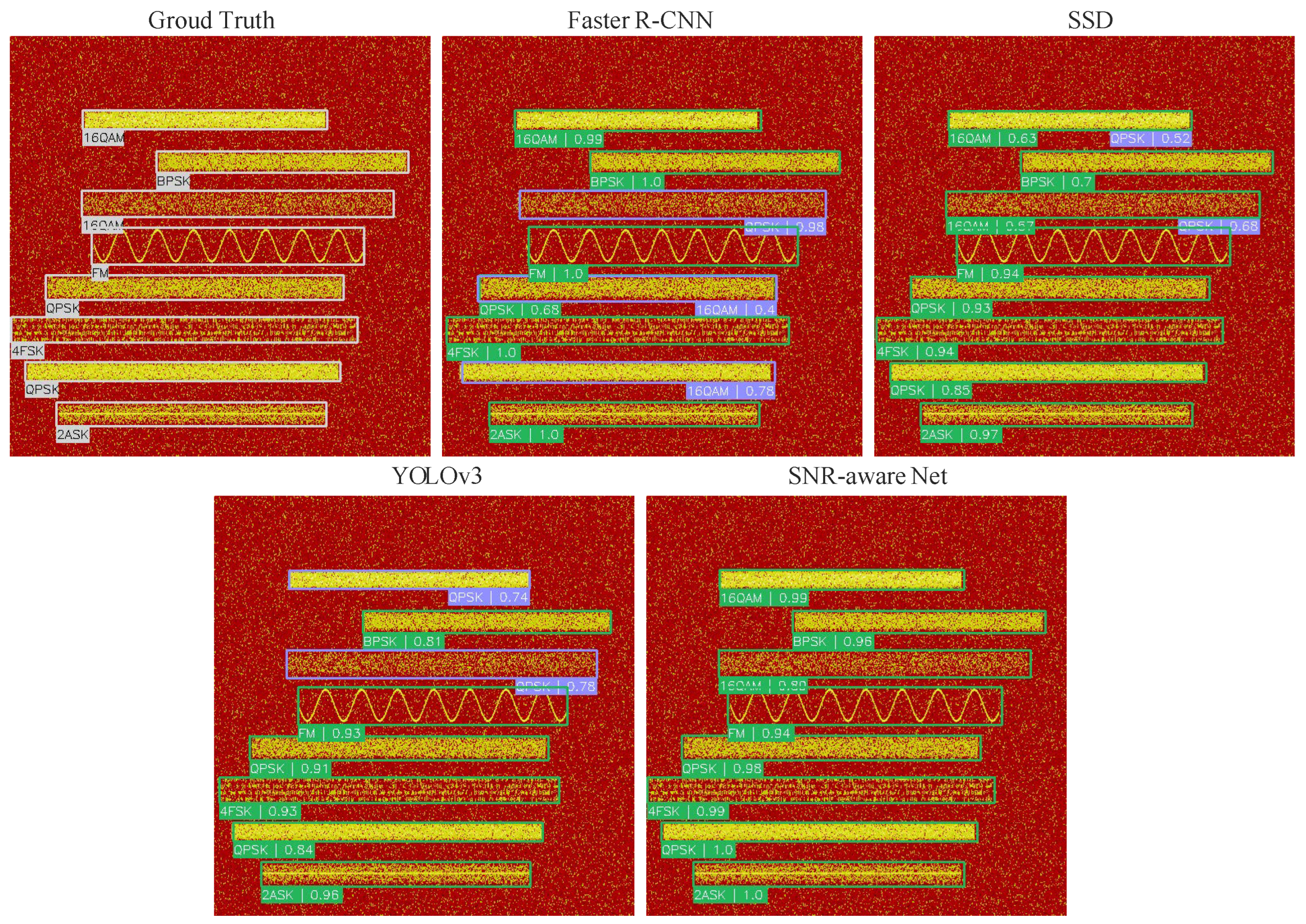
5.2.2. State-of-the-Art Comparisons of the Detection Networks

For the performance comparison of the networks, we first observe the superior mAP scores of SNR-aware Net in Table 2 when utilizing different spectrogram modalities as input. Despite the improvements brought by the MCE spectrogram to various networks, performance gaps still exist among them. Specifically, SNR-aware Net reports the best results, outperforming Faster R-CNN, SSD, and YOLOv3 by 3.8%, 10.3%, and 8% in terms of mAP, and by 3.2%, 7.7%, and 4.8% in terms of mAR, respectively.

To facilitate a clear comparison, we replot the performance versus SNR curves of the four networks with the MCE spectrogram as input in Figure 7. In terms of mAR, SNR-aware Net consistently outperforms the other networks at each SNR level. In terms of mAP, Faster R-CNN performs better when the SNR is below −5 dB. This superior performance of Faster R-CNN at low SNRs has been demonstrated in [5], as it is a two-stage region proposal-based network, which is well suited for signal localization and identification. Notably, despite all being one-stage networks, SNR-aware Net achieves significantly better performance than SSD and YOLOv3 at low SNRs through more task-oriented feature fusion and an efficient output paradigm, matching the performance of Faster R-CNN. When the SNR exceeds −5 dB, the mAP of SNR-aware Net is clearly the highest among the compared networks. To further investigate its superiority, we conduct further evaluations on the 5 dB subtest set.

First, we plot the precision–recall curves (PRCs) of the networks to visually compare their joint classification and localization performance, as shown in Figure 8. It is evident that the curve of SNR-aware Net consistently encloses the curves of the other networks for each signal class, indicating its superior ability to detect more signals with higher classification confidence and more precise regression.

Furthermore, we plot confusion matrices to visualize the classification performance of the four networks, as depicted in Figure 9. The rows represent the true classes, and the columns represent the predicted classes. The diagonal cells correspond to the correctly detected true positives (TPs). The last column represents background false negatives (FNs), which are missed GTs. The last row represents background false positives (FPs), which are detections predicted as a certain class but with IoUs below the threshold with all GTs. The other cells represent FPs, where the detection’s IoU with a certain GT exceeds the threshold, but the class does not match. As shown in the second row of Figure 9a, the detector misses 144 QPSK signals. Additionally, while correctly detecting 750 QPSK TPs, there are 558 16QAM FPs within the QPSK GT regions due to confusion between QPSK and 16QAM. A similar issue is observed in the fourth row, indicating that Faster R-CNN struggles to accurately distinguish between QPSK and 16QAM. Figure 9b,c show slight improvements achieved by SSD and YOLOv3, but they still exhibit poor recall and regression accuracy, leading to more background FNs and FPs. In contrast, Figure 9d demonstrates the superior performance of SNR-aware Net, which effectively differentiates each signal class and reduces misses and background FNs.

The results of SNR-aware Net indicate that using the MCE spectrogram as input is sufficient to distinguish different classes. However, as mentioned earlier, noise can impair feature extraction, and training ambiguity caused by feature misalignment can lead other networks to rely on less discriminative features, resulting in suboptimal performance. By contrast, SNR-aware Net achieves task-oriented feature fusion using TFFGAM and captures prior-knowledge-guided feature representations by introducing the SNR branch, thereby facilitating optimal performance. This demonstrates the effectiveness of the network and the overall framework as both a vision expert and a signal analysis specialist.

In addition, the visualization comparison of the detection results is presented in Figure 10. Corresponding to the confusion matrix, SNR-aware Net demonstrates superior performance by recalling all signals with higher confidence and precise regression. In contrast, the other networks produce more false positives (FPs) and misses because they do not capture feature representations with sufficient discrimination. Furthermore, the TP and FP predictions from these networks often have similar confidences and nearly identical coordinates, making it challenging to effectively filter out FPs by setting thresholds.

5.2.3. Complexity Comparisons

We conduct a complexity analysis on both the MCE spectrogram and SNR-aware Net, with the results listed in

Table 3. Complexity comparisons.

Detector	Parameters	Spectrogram Modality	Generation Time (ms)	Inference Time (ms)
		Grayscale spectrogram	14.024	142.4
Faster R-CNN	26.36M	RGB spectrogram	26.421	142.5
		MCE spectrogram	29.288	142.8
		Grayscale spectrogram	14.024	132.4
SSD	21.15M	RGB spectrogram	26.421	132.3
		MCE spectrogram	29.288	132.1
		Grayscale spectrogram	14.024	113.3
YOLOv3	61.57M	RGB spectrogram	26.421	113.6
		MCE spectrogram	29.288	113.1
		Grayscale spectrogram	14.024	44.6
SNR-aware Net	14.79M	RGB spectrogram	26.421	44.5
		MCE spectrogram	29.288	44.6

. These experiments were implemented on the Intel Core i5-10400F CPU and an NVIDIA Tesla K80 GPU, where we measure the average time per image over 1000 images.

First, we perform a quantitative comparison of the computational complexity among the three spectrograms, focusing on front-end generation speed and back-end inference speed. As shown in Table 3, the MCE and RGB spectrograms exhibit slightly increased generation times compared to the grayscale spectrogram. However, all three spectrograms demonstrate comparable inference speeds. For the MCE spectrogram, the slight increase in generation complexity is acceptable because the generation speed is still faster than the inference speed, thus having minimal impact on the overall processing speed during streaming data. Furthermore, we compare the complexity of the four networks in terms of network parameter size and inference speed. As shown in Table 3, SNR-aware Net is more lightweight, with fewer network parameters and faster inference speed.

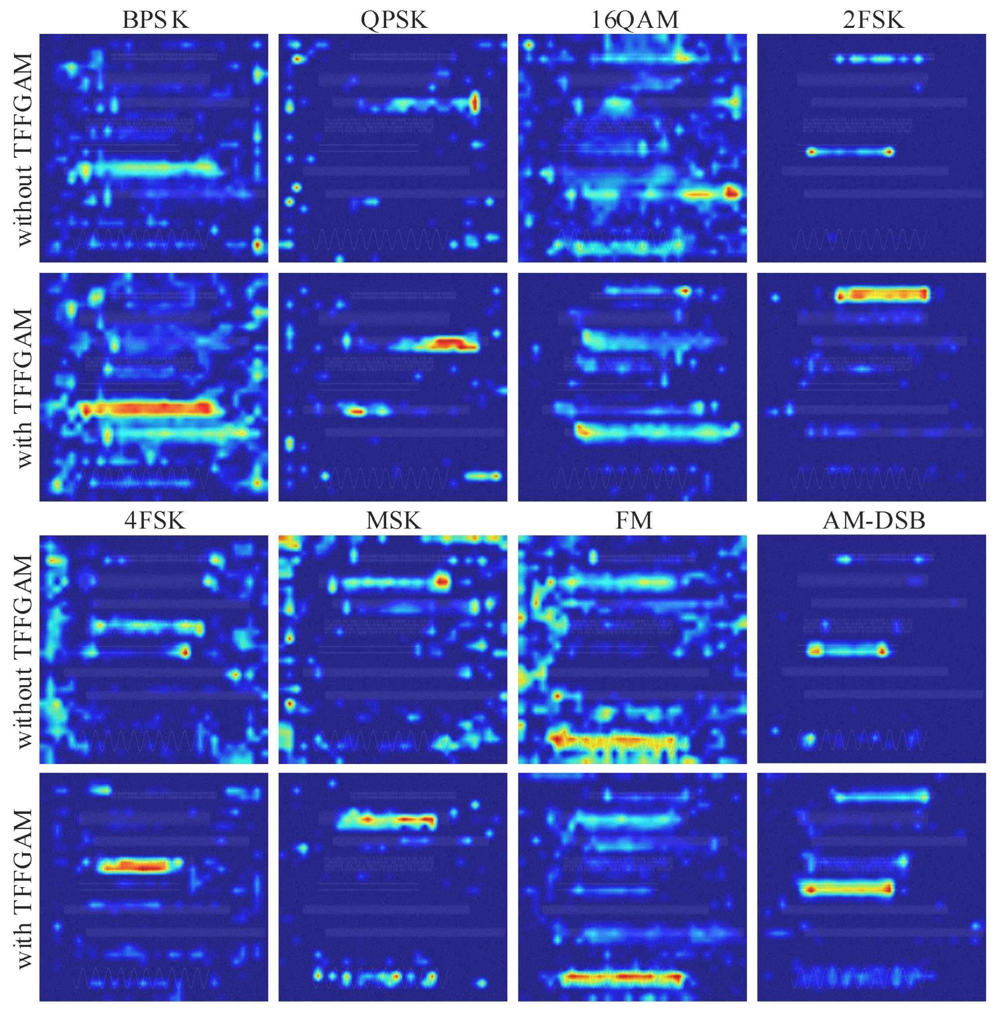
5.2.4. Ablation Experiments

The ablation experiments on the MCE spectrogram include channel ablation and threshold analysis, with the results listed in

Table 4. Ablation experiments of MCE spectrogram.

Channel 1	Channel 2	Channel 3	mAP (%)	mAR (%)
✔	×	×	71.9	84.1
×	✔($t_{75}$)	×	67.8	83.5
×	×	✔	71.7	84.6
✔	✔($t_{75}$)	×	76.3	87.5
✔	×	✔	75.5	86.5
✔	✔($t_{75}$)	✔	80.9	90.7
✔	✔($t_0$)	✔	76.1	87.1
✔	✔($t_{25}$)	✔	77.4	88.2
✔	✔($t_{50}$)	✔	79.5	89.4
✔	✔($t_{75}$)	✔	80.9	90.7
✔	✔($t_{100}$)	✔	75.5	86.5

. Regarding the channel ablation results, we first observe that using each individual channel as input results in suboptimal performance. Adding either the visual enhancement channel or the information complementary channel improves the performance. The greatest improvement is achieved when both channels are added. This demonstrates the complementary nature of the visual and informational enhancements provided by the MCE spectrogram, collectively leading to optimal performance. Next, due to memory constraints associated with dataset creation, we analyze the influence of different thresholds using five specific values. As shown in Table 4, $t_{75}$ is the optimal threshold among these. Excessively low or high thresholds adversely affect performance. The extreme cases of $t_0$ and $t_{100}$ indicate that the visual enhancement channel either degrades to the base channel or is zeroed out, both of which hinder effective visual enhancement and lead to poor attention guidance.

In addition,

Table 5. Ablation experiments of SNR-aware Net.

Method	TFFGAM	SNR Branch	mAP (%)	mAR (%)
Baseline	×	×	74.9	86.8
	✔	×	${78.6}_{+3.7}$	${89.2}_{+2.4}$
SNR-aware Net	×	✔	${77.3}_{+2.4}$	${87.9}_{+1.1}$
	✔	✔	${80.9}_{+6.0}$	${90.7}_{+3.9}$

presents the results of ablation experiments on SNR-aware Net. The SNR-aware Net without TFFGAM and the SNR branch is utilized as the baseline. It can be seen that the model with TFFGAM makes progress in precision while maintaining a higher recall. This improvement can be attributed to the trainable gating mechanism, which enables the network to capture visual and semantic feature combinations with better robustness and discrimination. We also visualize the feature patterns of the models with and without TFFGAM using Grad-CAM [40], as depicted in Figure 11. Grad-CAM leverages gradients to highlight the activation and contribution distribution of features. As can be seen, the model without TFFGAM exhibits scattered activations in regions that are not highly relevant to the specific categories being analyzed. In contrast, the model with TFFGAM shows more efficient feature patterns. Specifically, the areas that are most informative for the model’s predictions are strongly activated. These regions are crucial for identifying and localizing target signals. Furthermore, the responses from category-insensitive areas are effectively suppressed. Additionally, the inclusion of the SNR branch results in a 2.4% increase in mAP and a 1.1% increase in mAR. It optimizes the gradient backpropagation of the classification task, alleviates the feature misalignment during training, and further enhances the signal recognition performance. The full implementation of SNR-aware Net, including both TFFGAM and the SNR branch, achieves the best performance, with improvements of 6% for mAP and 3.9% for mAR.

We also explore the influence of different methods for categorizing SNR ranges. Initially, treating each SNR level as a separate class fails to converge effectively. By categorizing every five SNRs, we achieve an mAP of 79.9% and a mAR of 90.1%. Building on these results, we further consider the similarity of visual characteristics of signals at different SNRs and the performance versus SNR curves to determine the final categorization method, leading to further improvements.

6. Conclusions

In this paper, we propose an overall improved wideband signal detection framework that addresses the limitations of existing methods in both the front-end spectrogram and the back-end detection network. Firstly, we introduce a concise alternative, the MCE spectrogram, which outperforms the spectrogram baselines used in previous studies. The MCE spectrogram effectively enhances the performance of various networks while maintaining reasonable computational complexity. Secondly, we propose a novel anchor-free SNR-aware Net. This network not only achieves more efficient feature fusion through a trainable TFFGAM but also captures more prior-knowledge-guided feature representations by introducing an SNR branch. SNR-aware Net achieves state-of-the-art performance with fewer parameters and faster inference speed compared to other networks.

The distinctive contribution of this paper lies more in presenting a novel strategy to pursue optimal performance of the framework. Firstly, previous works have been overly network-centric, overlooking the importance of the front-end spectrogram. The superior performance of the MCE spectrogram demonstrates the effectiveness of enhancing the input modality. Secondly, previous works have been overly “visual”, ignoring task-specific distinctions and the supportive role of prior domain knowledge. The superior performance of SNR-aware Net suggests the potential for task-oriented modifications to the network. We also explore a promising method of incorporating prior knowledge into the network by introducing auxiliary tasks, which can be extended to other carefully designed branches to improve performance across diverse application scenarios. In future work, we will focus on expanding this strategy by exploring other types of TFRs at the front-end and utilizing channel-related prior knowledge to facilitate a more essential understanding of the signals by the back-end network.

References

1. Bhatti, F.A.; Khan, M.J.; Selim, A.; Paisana, F. Shared Spectrum Monitoring Using Deep Learning. IEEE Trans. Cogn. Commun. Netw. 2021, 7, 1171–1185. [Google Scholar] [CrossRef]
2. Soltani, N.; Chaudhary, V.; Roy, D.; Chowdhury, K. Finding Waldo in the CBRS Band: Signal Detection and Localization in the 3.5 GHz Spectrum. In Proceedings of the GLOBECOM 2022—2022 IEEE Global Communications Conference, Rio de Janeiro, Brazil, 4–8 December 2022; pp. 4570–4575. [Google Scholar]
3. Basak, S.; Rajendran, S.; Pollin, S.; Scheers, B. Combined RF-Based drone detection and classification. IEEE Trans. Cogn. Commun. Netw. 2021, 8, 111–120. [Google Scholar] [CrossRef]
4. Kayraklik, S.; Alagöz, Y.; Coşkun, A.F. Application of Object Detection Approaches on the Wideband Sensing Problem. In Proceedings of the 2022 IEEE International Black Sea Conference on Communications and Networking (BlackSeaCom), Sofia, Bulgaria, 6–9 June 2022; pp. 341–346. [Google Scholar]
5. Vagollari, A.; Schram, V.; Wicke, W.; Hirschbeck, M.; Gerstacker, W. Joint Detection and Classification of RF Signals Using Deep Learning. In Proceedings of the IEEE 93rd Vehicular Technology Conference (VTC-Spring), Helsinki, Finland, 25–28 April 2021; pp. 1–7. [Google Scholar]
6. Fonseca, E.; Santos, J.F.; Paisana, F.; DaSilva, L.A. Radio Access Technology characterisation through object detection. Comput. Commun. 2021, 168, 12–19. [Google Scholar] [CrossRef]
7. Zou, Z.; Chen, K.; Shi, Z.; Guo, Y.; Ye, J. Object Detection in 20 Years: A Survey. Proc. IEEE 2023, 111, 257–276. [Google Scholar] [CrossRef]
8. Prasad, K.S.; D’souza, K.B.; Bhargava, V.K. A Downscaled Faster-RCNN Framework for Signal Detection and Time-Frequency Localization in Wideband RF Systems. IEEE Trans. Wirel. Commun. 2020, 19, 4847–4862. [Google Scholar] [CrossRef]
9. Zha, X.; Peng, H.; Qin, X.; Li, G.; Yang, S. A deep learning framework for signal detection and modulation classification. Sensors 2019, 19, 4042. [Google Scholar] [CrossRef]
10. Li, R.; Hu, J.; Li, S.; Chen, S.; He, P. Blind Detection of Communication Signals Based on Improved YOLO3. In Proceedings of the 2021 6th International Conference on Intelligent Computing and Signal Processing (ICSP), Xi’an, China, 9–11 April 2021; pp. 424–429. [Google Scholar]
11. Prasad, K.S.; Dsouza, K.B.; Bhargava, V.K.; Mallick, S.; Boostanimehr, H. A Deep Learning Framework for Blind Time-Frequency Localization in Wideband Systems. In Proceedings of the 2020 IEEE 91st Vehicular Technology Conference (VTC2020-Spring), Antwerp, Belgium, 25–28 May 2020; pp. 1–6. [Google Scholar]
12. Zhao, R.; Ruan, Y.; Li, Y. Cooperative time-frequency localization for wideband spectrum sensing with a lightweight detector. IEEE Commun. Lett. 2023, 27, 1844–1848. [Google Scholar] [CrossRef]
13. Lin, M.; Tian, Y.; Zhang, X.; Huang, Y. Parameter Estimation of Frequency-Hopping Signal in UCA Based on Deep Learning and Spatial Time–Frequency Distribution. IEEE Sensors J. 2023, 23, 7460–7474. [Google Scholar] [CrossRef]
14. Yu, J.; Li, J.; Sun, B.; Chen, J.; Li, C. Multiclass Radio Frequency Interference Detection and Suppression for SAR Based on the Single Shot MultiBox Detector. Sensors 2018, 18, 4034. [Google Scholar] [CrossRef]
15. O’Shea, T.; Roy, T.; Clancy, T.C. Learning robust general radio signal detection using computer vision methods. In Proceedings of the 2017 51st Asilomar Conference on Signals, Systems, and Computers, Pacific Grove, CA, USA, 29 October–1 November 2017; pp. 829–832. [Google Scholar]
16. Ren, S.; He, K.; Girshick, R.; Sun, J. Faster R-CNN: Towards Real-Time Object Detection with Region Proposal Networks. IEEE Trans. Pattern Anal. Mach. Intell. 2017, 39, 1137–1149. [Google Scholar] [CrossRef]
17. Liu, W.; Anguelov, D.; Erhan, D.; Szegedy, C.; Reed, S.; Fu, C.Y.; Berg, A.C. SSD: Single Shot MultiBox Detector. In Computer Vision–ECCV 2016, Proceedings of the 14th European Conference, Amsterdam, The Netherlands, 11–14 October 2016; Springer: Cham, Switzerland, 2016; pp. 21–37. [Google Scholar]
18. Redmon, J.; Divvala, S.; Girshick, R.; Farhadi, A. You Only Look Once: Unified, Real-Time Object Detection. In Proceedings of the 2016 IEEE Conference on Computer Vision and Pattern Recognition (CVPR), Las Vegas, NV, USA, 27–30 June 2016; pp. 779–788. [Google Scholar]
19. Redmon, J.; Farhadi, A. YOLOv3: An Incremental Improvement. arXiv 2018, arXiv:1804.02767. [Google Scholar]
20. Liu, L.; Ouyang, W.; Wang, X.; Fieguth, P.W.; Chen, J.; Liu, X.; Pietikäinen, M. Deep Learning for Generic Object Detection: A Survey. Int. J. Comput. Vis. 2018, 128, 261–318. [Google Scholar] [CrossRef]
21. Lin, T.Y.; Goyal, P.; Girshick, R.; He, K.; Dollár, P. Focal Loss for Dense Object Detection. In Proceedings of the 2017 IEEE International Conference on Computer Vision (ICCV), Venice, Italy, 22–29 October 2017; pp. 2999–3007. [Google Scholar]
22. Zhang, X.; Zhao, H.; Zhu, H.; Adebisi, B.; Gui, G.; Gacanin, H.; Adachi, F. NAS-AMR: Neural Architecture Search-Based Automatic Modulation Recognition for Integrated Sensing and Communication Systems. IEEE Trans. Cogn. Commun. Netw. 2022, 8, 1374–1386. [Google Scholar] [CrossRef]
23. Li, L.; Dong, Z.; Zhu, Z.; Jiang, Q. Deep-Learning Hopping Capture Model for Automatic Modulation Classification of Wireless Communication Signals. IEEE Trans. Aerosp. Electron. Syst. 2023, 59, 772–783. [Google Scholar] [CrossRef]
24. Zhang, Z.; Wang, C.; Gan, C.; Sun, S.; Wang, M. Automatic Modulation Classification Using Convolutional Neural Network with Features Fusion of SPWVD and BJD. IEEE Trans. Signal Inf. Process. Over Netw. 2019, 5, 469–478. [Google Scholar] [CrossRef]
25. Behura, S.; Kedia, S.; Hiremath, S.M.; Patra, S.K. WiST ID—Deep Learning-Based Large Scale Wireless Standard Technology Identification. IEEE Trans. Cogn. Commun. Netw. 2020, 6, 1365–1377. [Google Scholar] [CrossRef]
26. O’Shea, T.J.; Roy, T.; Erpek, T. Spectral detection and localization of radio events with learned convolutional neural features. In Proceedings of the 2017 25th European Signal Processing Conference (EUSIPCO), Kos, Greece, 28 August–2 September 2017; pp. 331–335. [Google Scholar]
27. Sun, H.; Nallanathan, A.; Wang, C.X.; Chen, Y. Wideband spectrum sensing for cognitive radio networks: A survey. IEEE Wirel. Commun. 2013, 20, 74–81. [Google Scholar]
28. Gouldieff, V.; Palicot, J.; Daumont, S. Blind Modulation Classification for Cognitive Satellite in the Spectral Coexistence Context. IEEE Trans. Signal Process. 2017, 65, 3204–3217. [Google Scholar] [CrossRef]
29. Zhu, M.; Li, Y.; Pan, Z.; Yang, J. Automatic modulation recognition of compound signals using a deep multi-label classifier: A case study with radar jamming signals. Signal Process. 2020, 169, 107393. [Google Scholar] [CrossRef]
30. Zhang, M.L.; Zhou, Z.H. A Review on Multi-Label Learning Algorithms. IEEE Trans. Knowl. Data Eng. 2014, 26, 1819–1837. [Google Scholar] [CrossRef]
31. Yu, J.; Jiang, Y.; Wang, Z.; Cao, Z.; Huang, T. UnitBox: An Advanced Object Detection Network. In Proceedings of the 24th ACM international conference on Multimedia, MM ’16, Amsterdam, The Netherlands, 15–19 October 2016. [Google Scholar]
32. Rezatofighi, H.; Tsoi, N.; Gwak, J.; Sadeghian, A.; Reid, I.; Savarese, S. Generalized Intersection Over Union: A Metric and a Loss for Bounding Box Regression. In Proceedings of the 2019 IEEE/CVF Conference on Computer Vision and Pattern Recognition (CVPR), Long Beach, CA, USA, 15–20 June 2019; pp. 658–666. [Google Scholar]
33. Zheng, Z.; Wang, P.; Liu, W.; Li, J.; Ye, R.; Ren, D. Distance-IoU Loss: Faster and Better Learning for Bounding Box Regression. In Proceedings of the AAAI Conference on Artificial Intelligence, New York, NY, USA, 7–12 February 2020; Voume 34, pp. 12993–13000. [Google Scholar]
34. Han, K.; Wang, Y.; Tian, Q.; Guo, J.; Xu, C.; Xu, C. GhostNet: More Features From Cheap Operations. In Proceedings of the 2020 IEEE/CVF Conference on Computer Vision and Pattern Recognition (CVPR), Seattle, WA, USA, 14–19 June 2020; pp. 1577–1586. [Google Scholar]
35. Howard, A.G.; Zhu, M.; Chen, B.; Kalenichenko, D.; Wang, W.; Weyand, T.; Andreetto, M.; Adam, H. MobileNets: Efficient Convolutional Neural Networks for Mobile Vision Applications. arXiv 2017, arXiv:1704.04861. [Google Scholar]
36. He, K.; Zhang, X.; Ren, S.; Sun, J. Deep Residual Learning for Image Recognition. In Proceedings of the 2016 IEEE Conference on Computer Vision and Pattern Recognition (CVPR), Las Vegas, NV, USA, 27–30 June 2016; pp. 770–778. [Google Scholar]
37. Lin, T.Y.; Dollár, P.; Girshick, R.; He, K.; Hariharan, B.; Belongie, S. Feature Pyramid Networks for Object Detection. In Proceedings of the 2017 IEEE Conference on Computer Vision and Pattern Recognition (CVPR), Honolulu, HI, USA, 21–26 July 2017; pp. 936–944. [Google Scholar]
38. Zhou, X.; Wang, D.; Krähenbühl, P. Objects as Points. arXiv 2019, arXiv:1904.07850. [Google Scholar]
39. Padilla, R.; Passos, W.L.; Dias, T.L.; Netto, S.L.; Da Silva, E.A. A comparative analysis of object detection metrics with a companion open-source toolkit. Electronics 2021, 10, 279. [Google Scholar] [CrossRef]
40. Selvaraju, R.R.; Cogswell, M.; Das, A.; Vedantam, R.; Parikh, D.; Batra, D. Grad-CAM: Visual Explanations from Deep Networks via Gradient-Based Localization. In Proceedings of the 2017 IEEE International Conference on Computer Vision (ICCV), Venice, Italy, 22–29 October 2017; pp. 618–626. [Google Scholar]
Figure 1. Overview of the proposed framework. The dimensions 64 × 128 × 128 represent the number of channels, height, and width of the feature maps, respectively. The CBR unit refers to a convolution layer followed by a Batchnorm layer and an ReLU layer. The size of the convolution kernel is denoted as 1 × 1 , and C represents the amount of output channels from the convolution.
Electronics 14 02260 g001
Figure 2. An illustration of the MCE spectrogram.
Electronics 14 02260 g002
Figure 3. Histogram statistics of the matrix P c 1 generated from the same signal at (a) SNR = 10 dB, (b) SNR = 5 dB, (c) SNR = 0 dB, and (d) SNR = −10dB.
Electronics 14 02260 g003
Figure 4. Visual comparison of the three spectrograms at −5 dB SNR.
Electronics 14 02260 g004
Figure 5. Process of generating dataset and labels.
Electronics 14 02260 g005
Figure 6. Performance comparison versus SNR in combination with (a) Faster R-CNN, (b) SSD, (c) YOLOv3, and (d) SNR-aware Net.
Electronics 14 02260 g006
Figure 7. Performance comparison of detection networks with MCE spectrogram as input.
Electronics 14 02260 g007
Figure 8. PRC comparison of detection networks.
Electronics 14 02260 g008
Figure 9. Confusion matrix comparison of detection networks. (a) Faster R-CNN. (b) SSD. (c) YOLOv3. (d) SNR-aware Net.
Electronics 14 02260 g009
Figure 10. Visualization comparison of detection results. Green and purple boxes denote TPs and FPs, respectively.
Electronics 14 02260 g010
Figure 11. Visualization of feature maps produced by models with and without TFFGAM using Grad-CAM.
Electronics 14 02260 g011