MRNet: A Deep Learning Framework for Drivable Area Detection in Multi-Scenario Unstructured Roads

Abstract

In the field of autonomous driving, the accurate identification of drivable areas on roads is the key to ensuring the safe driving of vehicles. However, unstructured roads lack clear lane lines and regular road structures, and they have fuzzy edges and rutting marks, which greatly increase the difficulty of identifying drivable areas. To address the above challenges, this paper proposes a drivable area detection method for unstructured roads based on the MRNet model. To address the problem that unstructured roads lack clear lane lines and regular structures, the model dynamically captures local and global context information based on the self-attention mechanism of a Transformer, and it combines the input of image and LiDAR data to enhance the overall understanding of complex road scenes; to address the problem that detailed features such as fuzzy edges and rutting are difficult to identify, a multi-scale dilated convolution module (MSDM) is proposed to capture detailed information at different scales through multi-scale feature extraction; to address the gradient vanishing problem in feature fusion, a residual upsampling module (ResUp Block) is designed to optimize the spatial resolution recovery process of the feature map, correct errors, and further improve the robustness of the model. Experiments on the ORFD dataset containing unstructured road data show that MRNet outperforms other common methods in the drivable area detection task and achieves good performance in segmentation accuracy and model robustness. In summary, MRNet provides an effective solution for drivable area detection in unstructured road environments, supporting the environmental perception module of autonomous driving systems.

1. Introduction

Image segmentation tasks have benefited from the rapid development of deep learning technology and have been successfully applied to various fields including autonomous driving [1]. As an important part of the road perception task, drivable area recognition aims to automatically identify and segment road areas where vehicles can safely drive through computer vision and sensor data processing technology, providing support for the path planning, decision-making, and safe driving of autonomous vehicles [2]. In recent years, although drivable area recognition methods based on deep learning have been proven to be effective, image segmentation still faces many challenges in unstructured road scenarios [3]. Unstructured roads usually lack clear lane markings and regular road structures, and they face complex situations such as blurred edges and rutting, which makes it extremely difficult to accurately identify drivable areas.

Traditional image segmentation methods mainly rely on artificial feature extraction and rule-based models, such as edge detection and region-based segmentation methods. These methods work well in structured road scenes but are limited in unstructured road scenes due to insufficient understanding of complex scenes. With the development of deep learning technology, methods based on convolutional neural networks (CNNs) have been introduced into the field of image segmentation, significantly improving segmentation accuracy [4]. However, these methods still face problems such as inaccurate feature extraction and insufficient model generalization when dealing with unstructured road scenes. In recent years, multimodal data fusion has become an important direction for improving segmentation performance. By fusing multimodal data such as RGB images, LiDAR point clouds, and depth information, multimodal methods can not only utilize the powerful feature extraction capabilities of deep learning but also improve the robustness and accuracy of segmentation through the complementarity of multimodal data, and they can better cope with road segmentation tasks in complex environments [5].

In unstructured road scenarios, the existing research mainly focuses on how to improve the adaptability and segmentation accuracy of the model for complex scenarios. However, the existing methods still involve the problem of insufficient scene adaptability when dealing with complex roads with multiple scenes. In addition, due to the sparsity and computational complexity of the data, the performance of existing methods still needs to be improved when dealing with large-scale LiDAR scene data.

This paper proposes a drivable area detection method based on the MRNet model. MRNet adopts the Transformer architecture and enhances the understanding of complex road scenes by optimizing feature extraction and fusion mechanisms. This method improves the model’s robustness to edge blur and rutting interference through multi-scale feature extraction and residual learning mechanisms.

The contributions of this paper are summarized as follows:

• A deep learning framework based on the MRNet model is proposed for drivable area detection in a variety of unstructured road scenes, which enhances the understanding of complex road scenes.
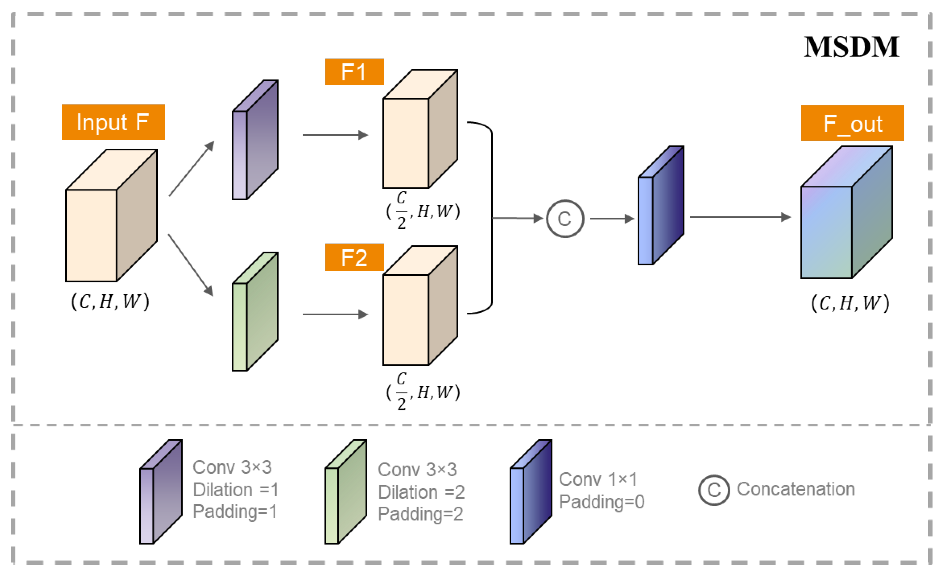
• The multi-scale dilated convolution module enables the model to capture features of different scales, so as to better adapt to complex scenes such as edge blur and rutting interference. This module significantly improves the adaptability of the model to complex scenes.
• The residual upsampling module effectively solves the gradient vanishing problem in feature fusion and further improves the segmentation accuracy. The residual upsampling mechanism learns the residual between input and output, enabling the network to propagate gradients more effectively and thereby improving training efficiency and model performance.

2. Related Work

2.1. Traditional Image Segmentation Methods

Traditional image segmentation methods primarily rely on manual feature extraction and rule-based models, such as edge detection and region-based segmentation techniques. Although these methods perform well in structured road scenes, their performance in unstructured road scenes is often limited due to the lack of understanding of complex scenes. For example, Alvarez et al. used thresholding and normalized histogram techniques to combine RGB images with enhanced grayscale images through a shadow-invariant feature space [6]. Chen et al. proposed using SIFT key features as the basis for motion region detection [7]. Slavkovic used Gabor wavelet transform to calculate texture information to extract drivable areas [8]. Bo Wang et al. developed a feature flow detection algorithm that extracts drivable areas in unstructured roads by aligning multiple frames and embedding motion features, combined with local geometric features (e.g., SIFT [9], HOG [10]), and effectively solves the problem of traditional grayscale segmentation failing under complex conditions such as shadow occlusion and road texture mutation [11]. However, these traditional methods are unstable when dealing with unstructured roads with blurred edges, showing obvious performance bottlenecks and a low upper limit of segmentation accuracy, which makes it difficult to meet the needs of high-precision applications.

2.2. Deep Learning-Based Image Segmentation Methods

With the advancement of deep learning technologies, convolutional neural network (CNN)-based methods have been introduced into the field of image segmentation, significantly enhancing segmentation accuracy [4]. For example, in the pixel-level segmentation task, FCN [12] replaces the initial fully connected layer with a full-scale layer, making it possible to process input images of any size and obtain segmentation results of the same size as the input. The emergence of U-Net [13] has become a new milestone. It uses an accurate encoder–decoder structure combined with skip connections to splice multi-pixel features, thereby improving boundary segmentation accuracy, especially for small sample scenarios such as medical images. The DeepLab series (including DeepLabv1, v2, v3, and v3+) further optimizes segmentation performance by introducing a hole model and multi-pixel features, solving the problem of blurred fusion segmentation boundaries [14,15,16,17]. DANet (Dual Attention Network) proposes a dual attention mechanism for space and channels, captures long-distance dependencies through a self-attention module, and achieves the best results on datasets such as Cityscapes and COCO Stuff [18]. Segformer proposed a simple Transformer-based semantic segmentation design that can capture both local and global context information, achieving state-of-the-art results on multiple efficient benchmarks [19]. Wang et al. proposed a high-resolution network (HRNet) that maintains spatial details through precision multi-resolution branches and achieved 83.5% mIoU on the Cityscapes dataset [20]. In addition, to address the challenges of rural road segmentation, such as irregular boundaries and simple boundary object types, researchers proposed an enhanced PP-LiteSeg model that contains novel modules such as SP-SPPM and B-UAFM to improve structure extraction and segmentation accuracy [21]. However, these methods still face the challenges of accurately extracting features and generalizing models when dealing with non-standardized path scenarios. For example, the performance of existing methods varies greatly under different signal conditions, seasonal changes, and meteorological conditions, maintaining stable segmentation accuracy.

2.3. Multimodal Data Fusion Methods

In recent years, multimodal data fusion has become an important direction for improving segmentation performance. By integrating multimodal data such as RGB images, LiDAR point clouds, and depth information, multimodal methods can not only utilize the powerful feature extraction capabilities of deep learning but also improve the robustness and accuracy of segmentation through the complementarity of multimodal data and better cope with road segmentation tasks in complex environments. For example, OFF-Net uses a Transformer-based architecture and a cross-attention module to fuse point cloud and image features, and it realizes the recognition of drivable areas in unstructured road scenes on the ORFD dataset [22]. Transfusion directly fuses images and point clouds for semantic segmentation without lossy preprocessing of point clouds [23]. BifNet first proposed a bidirectional fusion network, which realizes the spatial mapping between LiDAR point cloud bird’s-eye view (BEV) and camera images through dense spatial transformation modules combined with contextual feature fusion strategies, becoming a benchmark for early multimodal fusion methods [24]. SNE-RoadSeg combines RGB images with depth data (extracted by surface normal estimation) and uses an encoder–decoder architecture with dense skip connections to optimize feature fusion, demonstrating the robustness of multimodal data in complex lighting and occlusion scenarios [25]. AMFNet introduces an adaptive mask fusion module to dynamically adjust the weight distribution between RGB and depth data, effectively suppressing noise in unreliable areas (such as invalid pixels) in-depth images [26]. UdeerLID+ (2024) combines LiDAR point clouds, RGB images, and relative depth maps, combining semi-supervised learning with meta-pseudo-labeling technology to achieve high generalization capabilities with limited labeled data [27]. These studies provide important references for the recognition of drivable areas in unstructured road scenes. However, existing methods still face the challenge of adapting to different scenarios when dealing with complex roads in multiple scenarios. For example, under different lighting conditions, seasonal changes, and weather conditions, the performance of existing methods fluctuates greatly, making it difficult to maintain stable segmentation accuracy. Therefore, how to further improve the adaptability and robustness of the model in complex roads with multiple scenarios remains an urgent problem to be solved.

3. Methods

This section elaborates on the proposed drivable area detection method. Section 3.1 is the mathematical formulation of the drivable area detection problem. Section 3.2 outlines the proposed MRNet method. Section 3.3 describes the surface normal map generation process. Section 3.4 introduces the design of the encoder and decoder. Section 3.5 introduces the multi-scale dilated convolution module. Section 3.6 introduces the residual upsampling block. Finally, Section 3.7 introduces the loss function in detail.

3.1. Formulation of Drivable Area Detection Task

The task of drivable area detection can be formalized as a pixel-wise classification problem, with the goal of learning an optimal mapping function through the minimization of a loss function. Given an input image $I\in R^{H\times W\times C}$ and LiDAR data D, where $H, W,$ and $C$ denote the height, width, and number of channels of the image, respectively, the objective is to assign a class label, $y\in \{0,1\}$, to each pixel, where 0 represents the non-road area, and 1 represents the road area. This task can be achieved by learning an optimal mapping function, $f$, such that the output segmentation mask, $Y\in {\{0,1\}}^{H\times W}$, is as close as possible to the ground-truth labels, $Y^{*}$. Mathematically, this task can be expressed as follows:

$$Y=f(I; D; \theta )$$

(1)

where θ represents the model parameters. To optimize this mapping function, we define a loss function, L, to measure the discrepancy between the predicted results and the ground-truth labels. Specifically, our objective is to minimize the following loss function:

$${\mathit{min}}_{\theta }{\sum }_{i}L\left(F\right(I_i,D_i),Y_i^{*})$$

(2)

Here, $F(I_i,D_i)$ denotes the network’s prediction for the i-th sample, while $Y_i^{*}$ represents the ground-truth drivable area label for the i-th training sample. By minimizing this loss function, the model can learn to accurately identify drivable areas in unstructured road scenarios.

3.2. Methodology Overview

As shown in Figure 1, MRNet is built on an encoder–decoder framework based on the Transformer architecture, integrating cross-modal data inputs, including RGB images and surface normal maps. The input layer of the model receives RGB images and surface normal maps, where RGB images provide rich semantic information and surface normal maps provide geometric structure details. The resolution of the RGB image is 1280 × 720, and the surface normal map is calculated from the LiDAR point cloud data (see Section 3.3 for details) and aligned with the RGB image. The encoder is based on the Transformer architecture and enhances the capture of local and global information through a multi-scale feature extraction module. The residual upsampling module is integrated into the decoder to optimize the spatial resolution recovery process of the feature map and minimize feature loss. Finally, the model outputs a probability map with the same resolution as the input image, where each pixel value represents the possibility that the pixel belongs to a drivable area.

3.3. Surface Normal Map Generation

In the task of drivable road area recognition, the normal direction of the road surface usually has a certain similarity and can form a contrast with the normal direction of surrounding obstacles. Therefore, the surface normal map can serve as an effective feature to distinguish between road and non-road areas. The generation process of the surface normal map is described in Algorithm 1. For a perspective camera model, a point, P, in 3D space can be projected onto the 2D image plane through the camera intrinsic matrix, K, to form a pixel point, p. By using local plane fitting, combined with camera-intrinsic parameters and depth information, the horizontal and vertical gradients of the inverse depth image (1/D) can be calculated to approximately estimate the horizontal component,$n_x$, and vertical component, $n_y$, of the surface normal, n, of point P. This process is realized through convolution operations with horizontal and vertical gradient filters. In addition, neighborhood point information can be utilized to optimize the estimation of surface normals. Multiple normal estimates are calculated using neighboring points, and the optimal normal direction is found by minimizing the angle between these normals and the normalized normals of the neighborhood. The final surface normal direction is represented as a vector, $\widehat{n}={ [\mathit{sin}\theta \mathit{cos}\varphi , \mathit{sin}\theta \mathit{sin}\varphi , \mathit{cos}\theta ]}^T$, in spherical coordinates.

Algorithm 1: Surface normal map generation.

3.4. Encoder and Decoder Design

In the encoder stage, a Transformer-based architecture is employed to extract features from the input data. The Transformer architecture effectively captures both local and global contextual information through its multi-head self-attention and feed-forward neural network modules [28]. Specifically, the input data consists of RGB images and surface normal maps derived from LiDAR point clouds. To adapt these inputs to the Transformer architecture, we first apply patch embedding to both the RGB images and surface normal maps. This process segments the images and maps into smaller patches, which are then converted into tokenized sequences. These tokenized sequences are subsequently fed into a series of Transformer layers, each of which includes multi-head self-attention and feed-forward neural network modules, enabling deep feature extraction and transformation. We implement positional encoding using 3 × 3 convolution to enhance the model’s ability to capture global contextual information.

To further enhance the model’s ability to extract multi-scale features, the multi-scale dilated convolution module is introduced within the encoder. The MSDM utilizes dilated convolution layers with varying dilation rates to extract both fine-grained and coarse-grained features, generating a richer feature representation through feature fusion. The detailed design of MSDM will be elaborated upon in Section 3.5.

After feature extraction, a dynamic fusion module is employed to dynamically assign weights to the features from RGB images and surface normal maps, thereby fully leveraging the strengths of each modality. This module adds the features of RGB images and surface normal maps, and then it feeds the result into an MLP layer with a sigmoid activation function to learn the cross-attention. In this way, the features of each modality are dynamically weighted, effectively integrating the strengths of both modalities. The optimized feature calculation is as follows:

$$\begin{array}{c}Cros{s}_{\mathit{Attention}}=\sigma \left(X_{\mathit{im}{g}_{\mathit{in}}}+X_{s{n}_{\mathit{in}}}\right)\\ X_{\mathit{im}{g}_{\mathit{out}}}=Cros{s}_{\mathit{Attention}}*X_{\mathit{im}{g}_{\mathit{in}}}+X_{\mathit{im}{g}_{\mathit{in}}}\\ X_{s{n}_{\mathit{out}}}=\left(1-\mathit{Cros}{s}_{\mathit{Attention}}\right)*X_{s{n}_{\mathit{in}}}+X_{s{n}_{\mathit{in}}}\end{array}$$

(3)

Here, $X_{\mathit{im}{g}_{\mathit{in}}}$ and $X_{s{n}_{\mathit{in}}}$ represent the RGB image features and surface normal features learned through the Transformer module, respectively. $X_{\mathit{im}{g}_{\mathit{out}}}$ and $X_{s{n}_{\mathit{out}}}$ are the optimized RGB image features and surface normal features, respectively. σ denotes the sigmoid activation function. This dynamic fusion mechanism is placed at the end of the encoder to ensure that the features are effectively integrated and optimized before entering the decoder.

The Transformer decoder is used to integrate local and global information. The decoder consists solely of a multi-layer perceptron layer. Features extracted via the Transformer encoder are first fed into the multi-layer perceptron layer to aggregate channel-wise information and then upsampled to match the input size. To ensure the integrity of features during the upsampling process, residual connections are introduced in the decoder through the ResUp Block. The ResUp Block retains the original feature information via residual connections, thereby enhancing the continuity of features and detection accuracy. The detailed design of ResUp Block will be elaborated in Section 3.6. Finally, a pixel-level drivable area prediction probability map is generated through a multi-layer perceptron layer.

3.5. Multi-Scale Dilated Convolution Module

To enhance the model’s ability to extract multi-scale features, we introduce a multi-scale dilated convolution feature processing module after the encoder. This module uses two dilated convolution operations with different dilation rates to extract multi-scale deep features from the input data. The extracted features are then concatenated in the channel dimension and further fused through convolution operations to produce the final output. This design philosophy ensures that the core idea of multi-scale feature extraction is preserved while maintaining lightweight computational complexity and parameter count. By leveraging the advantages of dilated convolution, the module is able to capture contextual information across multiple scales, thereby enhancing the robustness and accuracy of road detection in complex scenes.

Dilated convolution is a convolution method proposed to address the problems of low image resolution and information loss in image semantic segmentation. It introduces a dilation rate parameter to control the distance between adjacent elements in the convolution kernel. By changing the dilation rate, the receptive field of the convolution kernel can be adjusted [14]. For a $k \times k$ convolution kernel, the output $\mathit{Out}(i,j)$) at position ($i,j$) of the dilated convolution can be expressed as follows:

$$\mathit{Out}(i,j)={\sum }_{m=0}^{k\mathit{-}1}{\sum }_{n=0}^{k\mathit{-}1}\mathit{Kernel}(m,n)\times \mathit{Input}(i+m\times d,j+n\times d)$$

(4)

where $\mathit{Out}(i,j)$ is the value of the output feature map at position ($i,j$), $\mathit{Kernel}(m,n)$ is the value of the convolution kernel at position $(m,n)$, $\mathit{Input}(i+m \times d, j+n \times d)$ is the value of the input feature map at position $(i+m \times d, j+n \times d)$, and $d$ is the dilation rate, which controls the spacing between sampled points in the convolution kernel.

In traditional convolution operations, the elements of the convolution kernel are contiguous. In contrast, dilated convolution introduces spacing in the convolution kernel, enabling it to cover a larger spatial range. This enables the convolution kernel to capture more contextual information and enhances the model’s ability to perceive local details and global information. For the task of drivable area recognition on unstructured roads, it is particularly important to expand the receptive field to capture more contextual information. This is because road edges usually have complex shapes and are easily affected by interference such as shadows and rutting.

In the MRNet model, MSDM is introduced at different stages of the encoder (Stage 1 to Stage 4). By employing parallel dilated convolutional layers with dilation rates of 1 and 2, respectively, the MSDM captures both local details and global information. This design maintains the resolution of the feature maps and generates denser feature responses, thereby enriching the details when the features are upsampled back to the original image resolution.

Given an input feature map, F, with dimensions $H \times W \times C$ (where $H$ is the height, $W$ is the width, and $C$ is the number of channels), the MSDM first extracts multi-scale features through two parallel dilated convolutional layers. The outputs of these two dilated convolutional layers can be represented as follows:

$$\begin{array}{c}{F}_1 ={\mathit{Conv}}_{3\times 3}^{d=1}\left(F\right)\\ F_2={ \mathit{Conv}}_{3\times 3}^{d=2}\left(F\right)\end{array}$$

(5)

Here, $F_1$ and $F_2$ are the feature maps obtained from the dilated convolutional layers with dilation rates of 1 and 2, respectively. These feature maps capture different scales of contextual information, with $F_1$ focusing on finer details and $F_{2 }$capturing broader contextual information.

The choice of dilation rates 1 and 2 is based on the mathematical properties of dilated convolutions and their impact on feature extraction. A dilation rate of 1 corresponds to a standard convolution operation, which captures fine-grained details. A dilation rate of 2 doubles the receptive field size, allowing the convolution kernel to cover a larger spatial range and capture more contextual information. This combination ensures that the model can effectively capture both local and global features.

After obtaining $F_{1 }$ and $F_2$, the MSDM typically combines these feature maps through concatenation along the channel dimension, followed by a convolutional layer to fuse the multi-scale features into a single output feature map. The combined feature map can be represented as follows:

$$F_{\mathit{out} }={\mathit{Conv}}_{1\times 1}\left(\mathit{Concat}\right(F_{1 },F_2\left)\right)$$

(6)

where $F_{\mathit{out} }$ is the final output feature map of the MSDM. This output feature map is then used as input for the subsequent stages of the MRNet model.

By incorporating the MSDM at different stages of the encoder, the MRNet model is able to effectively capture both local and global contextual information, enhancing its performance in tasks such as road segmentation and object detection.

As shown in Figure 2, the specific structure of the MSDM is presented. It focuses on extracting multi-scale information by introducing multiple stacked dilated convolutional branches in the encoder. This approach enhances the local details of multi-scale features, thereby enabling the model to continuously compute spatial information and strengthening its ability to capture multi-scale information.

3.6. Residual Upsampling Block

In the task of drivable area detection on unstructured roads, the upsampling module is a crucial component of the decoder, responsible for restoring the spatial resolution of feature maps and thereby providing richer detail information for the final segmentation results. However, traditional upsampling methods often suffer from feature loss in deep networks, which can affect the model’s detection accuracy and robustness [29]. To address this issue, this study introduces a Residual-Enhanced Upsampling Module in the decoder of MRNet, which enhances the upsampling process through residual connections, ensuring the integrity and continuity of feature information.

As shown in Figure 3, the detailed structure of the ResUp Block is presented. Its core concept is to optimize the feature transmission and restoration process by combining residual connections with upsampling convolution operations.

In the resup block, the upsampling module employs a bilinear interpolation strategy to upsample feature maps from different stages of the encoder to the same resolution as the highest-resolution feature map. Compared with transposed convolution, bilinear interpolation is more computationally efficient and can effectively retain contextual information through feature fusion mechanisms [30].

After the upsampling module, the feature maps from the four branches are concatenated and then passed through a 1 × 1 convolution to compress the channel dimension. This fusion mechanism integrates the semantic information of multi-scale features, providing more comprehensive contextual perception for subsequent segmentation tasks. Assuming the upsampled features from the four branches are $F_{c4}$, $F_{c3}$, $F_{c2}$, and $F_{c1}$, the fused feature $F_{\mathit{fuse}}$ can be represented as follows:

$${ F}_{\mathit{fuse}}={ \mathit{Conv}}_{1\times 1}\left(\mathit{Concat}\left(F_{c4},F_{c3},F_{c2},F_{c1}\right)\right)$$

(7)

In Equation (7), $\mathit{Concat}$ denotes the channel concatenation operation, and ${ \mathit{Conv}}_{1\times 1}$ represents the 1 × 1 convolution operation used to adjust the number of channels.

To further optimize feature transmission, the ResUp Block introduces a residual connection mechanism [31]. The residual connection is designed to address the common vanishing gradient problem in deep neural networks. In deep networks, gradients may diminish during backpropagation, making it difficult to update the weights of early layers. The residual connection is based on the principle of learning the residual between the input and output of a network layer. Specifically, the residual connection can be expressed as follows:

$$H\left(x\right)=F\left(x\right)+x$$

(8)

where $H\left(x\right)$ is the output of the network layer, $F\left(x\right)$ is the residual function, and $x$ is the input. This form ensures that gradients can directly flow through the residual connection, reducing the risk of vanishing gradients.

By directly adding the input $x$ to the output $F\left(x\right)$, gradients can flow directly through the residual connection during backpropagation. This direct path ensures that gradients do not vanish as they pass through the network, thereby improving training efficiency and stability. Moreover, the residual connection helps maintain the integrity and continuity of feature information during upsampling. In deep networks, complexity can lead to feature loss.

The ResUp Block addresses this by adding the original input feature C₁, after adjusting its channel number through a 1 × 1 convolution, to the fused feature ${ F}_{\mathit{fuse}}$. This process retains the detail information of the original features and alleviates the vanishing gradient problem. The residual connection operation can be expressed as follows:

$$F_{\mathit{out}}=F_{\mathit{fuse}}+{\mathit{Conv}}_{1\times 1}\left(C_1\right)$$

(9)

The final output feature $F_{\mathit{out}}$ is used for subsequent segmentation tasks. By introducing residual connections, the ResUp Block not only preserves the upsampled feature information but also enhances the feature representation ability, thereby improving the model’s adaptability to complex scenarios.

3.7. Loss Function

In this study, to enhance the performance of the drivable area detection model in unstructured road environments, we employed the binary cross-entropy loss function as the optimization criterion for model training. This loss function provides an effective learning signal for the model by quantifying the logarithmic likelihood difference between the model’s predicted outputs and the true labels. Specifically, the calculation of the loss function is as follows:

$$L\mathit{oss}={\displaystyle \frac{\mathit{-}1}{bs}}\sum _{i=0}^{bs}\sum _{m=1}^M\sum _{n=1}^N{\widehat{Y}}_{\mathit{mn}}^i\mathit{log}{O}_{\mathit{mn}}^i$$

(10)

where $O_{\mathit{mn}}^i$ represents the predicted probability of the pixel (m,n) in the i-th training sample, and ${\widehat{ Y}}_{\mathit{mn}}^i$ denotes the corresponding true label. This loss function only calculates for pixels labeled as drivable areas (i.e., ${\widehat{Y}}_{\mathit{mn}}^i$ = 1), thereby ensuring that the model focuses on improving the recognition accuracy of these regions.

By minimizing the binary cross-entropy loss function, the model is incentivized to learn how to more accurately distinguish between drivable and non-drivable areas. This approach not only enhances the model’s identification capability for drivable areas but also improves the model’s robustness in complex road scenarios. The binary cross-entropy loss function is particularly suitable for pixel-level classification tasks because it directly optimizes the classification results of each pixel, thus providing precise guidance for the adjustment of model parameters.

Furthermore, the design of this loss function ensures that the model can balance the impact of positive and negative samples during the training process, thus finding an optimal decision boundary between drivable and non-drivable areas. In this way, the model can more effectively learn from the differences between predicted results and true labels and gradually adjust parameters through gradient descent algorithms to reduce these differences, thereby enhancing the model’s recognition and generalization capabilities.

4. Experiments

In this section, we conduct a thorough analysis of the experimental results of our proposed drivable area detection method. Section 4.1 outlines the implementation details, including the experimental environment and training parameter settings. Section 4.2 provides a detailed description of the datasets and evaluation metrics. In Section 4.3, we present the quantitative assessment of our model’s performance and compare it with other state-of-the-art approaches. Section 4.4 includes qualitative evaluations, showcasing example results that demonstrate the effectiveness of our method. Additionally, to gain insights into the contributions of different components of our model, we conduct ablation studies in Section 4.5. These studies help to validate the significance of each part of the model in achieving overall detection performance.

4.1. Implementation Details

The hardware configuration employed in the experiment includes two Nvidia RTX 4090 GPUs (Nvidia Corporation, Santa Clara, USA), which provide substantial computational performance to accelerate the training and inference processes of the model. The software environment is based on the PyTorch deep learning framework (version 1.10.0), in conjunction with Python 3.8, CUDA 11.3, and the Ubuntu 20.04 operating system. This setup offers the necessary support for efficient model training and stable inference.

During the model training process, we utilized a deep learning model and optimized the key hyperparameters. The optimizer chosen was Stochastic Gradient Descent with Momentum (SGDM), with an initial learning rate set at 0.001. A dynamic learning rate adjustment strategy was also implemented. Specifically, a learning rate scheduler with ‘lr_policy = ‘lambda’’ was used, and the learning rate was updated by multiplying it with a preset decay factor of 0.9 every 25 epochs. Additionally, to further expedite model convergence and enhance training stability, the momentum parameter was set to 0.5, and the weight decay coefficient was set to 0.0005 to prevent overfitting and ensure the robustness of the model in complex data environments.

4.2. Datasets and Evaluation Metrics

The experiments in this paper utilized the ORFD dataset. As illustrated in Figure 4, in terms of scene categories, the dataset encompasses diverse unstructured road scenes, including farmland, countryside, woodland, and grassland. Regarding weather conditions, it covers a variety of scenarios for autonomous vehicle navigation, such as sunny, rainy, foggy, and snowy days. In terms of illumination intensity, the dataset includes conditions ranging from bright light to daylight, twilight, and darkness. From the perspective of data modality, the dataset comprises both image and LiDAR point cloud data. The LiDAR is a 40-line mechanical rotating LiDAR that generates 3D images through 360° rotation with 40 internal laser diodes. It has a measurement range of up to 200 m at 20% reflectivity and can generate up to 720,000 data points per second. The ORFD dataset contains a total of 12,198 pairs of LiDAR point clouds and images. Annotations are provided from the image perspective, distinguishing between traversable and non-traversable areas. For the annotation of LiDAR data, a method similar to that of the KITTI dataset is employed, where LiDAR point clouds are projected onto an RGB image plane to obtain depth information.

Evaluation metrics: To comprehensively evaluate the performance of segmentation methods, we utilized seven commonly employed metrics: accuracy, precision, recall, F1-score, intersection over union (IoU), params, and inference time [32,33,34]. Accuracy measures the proportion of correctly classified pixels out of the total number of pixels in the dataset. Precision reflects the proportion of correctly identified positive pixels among all pixels classified as positive. Recall indicates the proportion of correctly identified positive pixels among all actual positive pixels. F1-score is the harmonic mean of precision and recall, providing a balanced measure of the two. IoU measures the overlap between the predicted segmentation mask and the ground-truth mask, calculated as the ratio of the intersection area to the union area of the two masks. Params represent the model’s parameter count, indicating its complexity and computational resource demand. Fewer parameters mean a lighter model, easier to deploy on resource-limited devices. Inference time is the time required to process a frame of data, reflecting the model’s speed in practical applications. The shorter the inference time, the faster the model processes each frame, enhancing real-time performance.

4.3. Quantitative Evaluation

To comprehensively evaluate the performance of MRNet in the task of traversable region recognition in unstructured roads, extensive comparative experiments were conducted. MRNet was benchmarked against four other prevalent road segmentation methods, encompassing both CNN-based and Transformer-based architectures, namely FuseNet, SNE-RoadSeg, AMFNet, and OFF-Net.

As illustrated in

Table 1. Quantitative results on the ORFD dataset.

Title 1	Accuracy	Precision	Recall	F1-Score	IoU	Params	Inference Time
FuseNet [35]	0.874	0.745	0.852	0.795	0.660	50 M	20.4 ms
SNE-RoadSeg [25]	0.938	0.867	0.927	0.896	0.812	201.3 M	80 ms
AMFNet [26]	0.943	0.907	0.920	0.905	0.836	183.9 M	55.6 ms
OFF-Net [22]	0.946	0.892	0.942	0.916	0.845	25.2 M	29.5 ms
MRNet	0.957	0.918	0.923	0.921	0.853	29 M	31.2 ms

, MRNet demonstrates superior performance across multiple key metrics compared to the other four methods. Specifically, MRNet achieves an accuracy of 0.957, a precision of 0.918, a recall of 0.923, an F1-score of 0.921, and an intersection over union (IoU) of 0.853. These results strongly indicate that MRNet can segment drivable areas with higher precision in complex scenarios. Additionally, MRNet’s inference time is 31.2 ms, which, although slightly higher than OFF-Net’s 29.5 ms, is significantly better compared to AMFNet and SNE-RoadSeg, demonstrating good real-time performance. Moreover, with a parameter count (Params) of 29 M, MRNet is only slightly higher than OFF-Net’s 25.2 M but far less than AMFNet’s 183.9 M and SNE-RoadSeg’s 201.3 M. This shows that MRNet maintains high performance while having a lower model complexity, making it more suitable for deployment on resource-constrained devices.

In order to further verify the robustness of our model under different environmental conditions, we have meticulously classified the images in the dataset based on weather conditions and light intensity, and we evaluated the model’s performance under these specific conditions. The distribution of the dataset is shown in

Table 2. Dataset distribution based on weather and light conditions.

Dataset	Weather Condition				Light Condition
	Sunny	Rainy	Foggy	Snowy	Bright Light	Daylight	Twilight	Darkness
Train	3803	2434	1136	1025	1019	4254	927	2198
Val	356	302	0	587	0	356	302	587
Test	1071	405	720	359	362	709	359	1125

.

The performance of the proposed MRNet under different weather conditions (sunny, rainy, foggy, and snowy) and light intensities (strong light, daylight, twilight, and darkness) is shown in

Table 3. Performance of MRNet across different weather and light conditions.

Condition		Accuracy	Precision	Recall	F1-Score	IoU
Weather	Sunny	0.976	0.98	0.924	0.961	0.924
	Rainy	0.954	0.871	0.896	0.879	0.778
	Foggy	0.946	0.875	0.942	0.924	0.861
	Snowy	0.932	0.869	0.958	0.883	0.793
Light	Bright light	0.955	0.966	0.88	0.944	0.853
	Daylight	0.977	0.987	0.914	0.972	0.936
	Twilight	0.941	0.869	0.942	0.884	0.785
	Darkness	0.955	0.911	0.927	0.92	0.857

.

The results in Table 3 show that MRNet performs well under a variety of light and weather conditions. However, under extreme conditions such as twilight, rainy weather, and snowy weather, the model’s precision and IoU metrics significantly decrease. This indicates that adverse weather conditions interfere with the data from the LiDAR and cameras, thereby affecting the model’s performance. Although MRNet demonstrates high robustness and generalization ability in complex environments, there is still room for improvement in its performance under extreme weather conditions.

4.4. Ablation Studies

To systematically evaluate the contributions of different components in our model, we conducted comprehensive ablation experiments on the ORFD dataset, and the results are summarized in

Table 4. Performance for different component combinations of our model.

MSDM	ResUp Block	Accuracy	Precision	Recall	F1-Score	IoU
-	-	0.946	0.892	0.942	0.916	0.845
√	-	0.952	0.909	0.915	0.916	0.852
-	√	0.954	0.910	0.923	0.923	0.847
√	√	0.957	0.918	0.923	0.921	0.853

and visualized in Figure 5.

As shown in Table 4, the introduction of the multi-scale feature module (MSDM) and the residual upsampling module alone and in combination can improve the performance of the model. Specifically, the introduction of the MSDM alone improves the intersection over union (IoU) from 0.845 to 0.852 and the precision from 0.892 to 0.909, which shows that MSDM has a significant effect in capturing multi-scale features and enhancing the adaptability of the model to complex scenes. The introduction of the ResUp Block alone improves the precision by 0.018 and the IoU by 0.002, which shows that the residual connection mechanism significantly reduces feature loss and optimizes the upsampling process of the feature map. When the MSDM and ResUp Block are introduced at the same time, the model achieves the highest performance, with an accuracy of 0.957, a precision of 0.918, a recall of 0.923, an F1 score of 0.921, and an IoU of 0.853. This shows that the combination of these components produces a synergistic effect, further enhancing the model’s ability to capture detailed features and improving the overall segmentation accuracy.

To further explore the synergy between MSDM and ResUp Block in different scenarios, we conducted additional experiments under different weather and lighting conditions. We plotted a radar chart (Figure 5) to visually compare the performance of different module combinations across these scenarios.

As can be seen from Figure 5, the combination of MSDM and ResUp Block generally demonstrates superior performance compared to the individual modules and the original model in most metrics. The MSDM primarily enhances the model’s ability to capture multi-scale features, which is crucial for identifying drivable areas in complex scenes with varying levels of detail. However, this enhancement in precision comes at the cost of a slight reduction in recall. This trade-off suggests that while the model becomes more precise in identifying drivable areas, it may miss some true positive cases, likely due to the increased focus on fine details and the suppression of false positives.

Conversely, the ResUp Block significantly improves accuracy, precision, and F1-score, with a minor increase in recall. By enhancing the feature transmission and restoration process through residual connections, the ResUp Block ensures the integrity and continuity of feature information, thereby reducing feature loss during the upsampling process.

When MSDM and ResUp Block are combined, the model’s performance is further enhanced across all metrics. This combination not only improves precision and IoU but also maintains a balanced recall, leading to a higher F1-score and overall accuracy. The strengths of the two modules complement each other, resulting in a more robust and accurate model. This indicates that the synergy between MSDM and ResUp Block is effective in enhancing the model’s performance across various conditions.

4.5. Qualitative Evaluation

As mentioned in the quantitative analysis above, MRNet shows excellent performance in the task of identifying drivable areas on unstructured roads, and the module proposed in this paper improves the accuracy of the model. Figure 6 shows the visualization results of MRNet on the ORFD dataset. From left to right, the figure shows two input modes: RGB image and surface normal map, as well as the predicted probability map and the final road segmentation result superimposed on the original image. It can be intuitively observed that under various lighting and weather conditions, MRNet can accurately identify the drivable area of the road.

In addition, open-pit mine road scenes are also common unstructured road scenes. Open-pit mine roads have the characteristics of blurred boundaries between roads and terrain, unclear road edges, and large spatial three-dimensional coordinate spans, which makes the identification of drivable areas in open-pit mines more challenging. The visualization results of the proposed method on open-pit mine roads are shown in Figure 7. As can be seen from the figure, the MRNet proposed in this paper can accurately identify the drivable areas on mine roads, which shows that the model has a certain generalization ability. It shows that MRNet not only performs well on the ORFD dataset, but can also adapt to more complex and challenging open-pit mine environments.

5. Discussion and Conclusions

5.1. Summary of Research Contributions

This study proposes a drivable area detection method for unstructured roads based on the MRNet model. The model integrates a multi-scale feature extraction module (MSDM) and a residual upsampling block (ResUp Block), which enhances the detection performance of drivable areas in complex unstructured road scenes. The MSDM effectively captures multi-scale features and enhances the model’s adaptability to complex scenes, while the ResUp Block significantly reduces feature loss through residual connections and optimizes the upsampling process of feature maps. Extensive experiments on the ORFD dataset have shown that MRNet outperforms other common methods in key metrics such as accuracy, precision, F1 score, and intersection over union (IoU). Specifically, MRNet achieved values of 0.957, 0.918, 0.921, and 0.853 in these metrics, respectively. In terms of performance, MRNet has an inference time of 31.2 ms and a parameter count of 29 M. By maintaining a low number of parameters, it achieves a short inference time, making MRNet more suitable for real-time application deployment on resource-constrained devices. Moreover, MRNet not only performs well on the standard test set but also demonstrates good generalization ability in open-pit mine road scenarios. In summary, MRNet provides a new approach for drivable area recognition in unstructured road scenes and supports the safe navigation of autonomous vehicles in complex environments.

5.2. Future Work Outlook

Although the current study has demonstrated the effectiveness of MRNet in drivable area detection, many challenges remain in practical applications. Future work will focus on the following two aspects to further enhance the performance and practicality of MRNet:

Impact of image quality and environmental factors. The performance of MRNet may be affected by a combination of factors such as image resolution, noise levels, rut depth, and lighting conditions. Low-resolution, high-noise images, and deep ruts in complex road conditions can all weaken the model’s detection accuracy of drivable areas. To address these challenges, future research will introduce advanced image preprocessing techniques, such as denoising algorithms and super-resolution methods, to enhance the robustness of MRNet to low-quality images. Additionally, collecting and annotating data that includes rut depth information will provide richer samples for model training and enhance the model’s understanding and recognition of complex road conditions, thereby further improving its adaptability in complex environments.

Practical deployment and hardware compatibility. Practical deployment is also a key focus for future research. Deploying MRNet in actual autonomous vehicles requires consideration of computational resource demands and hardware compatibility. The current computational complexity and inference time of the model need to be optimized to ensure efficient operation on the vehicle’s computing platform. To this end, future research will explore hardware acceleration options, such as dedicated GPUs or FPGAs, to significantly improve the real-time performance of MRNet. This will involve optimizing the model architecture for specific hardware platforms and exploring the use of specialized computing units to reduce latency and increase efficiency. Additionally, further optimization of the model architecture, exploration of lightweight alternatives, investigation of the impact of vehicle speed on computation time and GPU usage, and adaptation to the computational resource limitations of on-board hardware will be explored to enhance its efficiency and adaptability in practical applications.

In summary, while MRNet performs well in detecting drivable areas in unstructured road scenes, further in-depth research is needed in practical autonomous driving applications to address the impact of image quality and environmental factors and to facilitate practical deployment. Future work will focus on enhancing the robustness of the model to low-quality images and complex environmental conditions (including rut depth and changes in lighting conditions), expanding the dataset with depth information annotations, optimizing the model architecture to accommodate the computational resource limitations of on-board hardware, and exploring hardware acceleration technologies to ensure real-time performance. Through these efforts, we expect MRNet to demonstrate higher feasibility and effectiveness in complex real-world scenarios, providing strong support for the development of autonomous driving technology.

References

1. Minaee, S.; Boykov, Y.Y.; Porikli, F.; Plaza, A.J.; Kehtarnavaz, N.; Terzopoulos, D. Image Segmentation Using Deep Learning: A Survey. IEEE Trans. Pattern Anal. Mach. Intell. 2022, 44, 3523–3542. [Google Scholar] [CrossRef] [PubMed]
2. Wang, Q.; Lyu, C.; Li, Y. A Method for All-Weather Unstructured Road Drivable Area Detection Based on Improved Lite-Mobilenetv2. Appl. Sci. 2024, 14, 8019. [Google Scholar] [CrossRef]
3. Shang, E.; An, X.J.; Li, J.; Ye, L.; He, H.G. Robust Unstructured Road Detection: The Importance of Contextual Information. Int. J. Adv. Robot. Syst. 2013, 10, 179. [Google Scholar] [CrossRef]
4. LeCun, Y.; Bengio, Y.; Hinton, G. Deep learning. Nature 2015, 521, 436–444. [Google Scholar] [CrossRef]
5. Zhang, Y.; Sidibé, D.; Morel, O.; Mériaudeau, F. Deep multimodal fusion for semantic image segmentation: A survey. Image Vis. Comput. 2021, 105, 104042. [Google Scholar] [CrossRef]
6. Alvarez, J.M.; Lopez, A.M. Road Detection Based on Illuminant Invariance. IEEE Trans. Intell. Transp. Syst. 2011, 12, 184–193. [Google Scholar] [CrossRef]
7. Chen, C.C.; Lu, W.Y.; Chou, C.H. Rotational copy-move forgery detection using SIFT and region growing strategies. Multimed. Tools Appl. 2019, 78, 18293–18308. [Google Scholar] [CrossRef]
8. Slavkovic, N.; Bjelica, M. Risk prediction algorithm based on image texture extraction using mobile vehicle road scanning system as support for autonomous driving. J. Electron. Imaging 2019, 28, 033034. [Google Scholar] [CrossRef]
9. Lowe, D.G. Distinctive image features from scale-invariant keypoints. Int. J. Comput. Vis. 2004, 60, 91–110. [Google Scholar] [CrossRef]
10. Dalal, N.; Triggs, B. Histograms of oriented gradients for human detection. In Proceedings of the Conference on Computer Vision and Pattern Recognition, San Diego, CA, USA, 20–25 June 2005; pp. 886–893. [Google Scholar]
11. Wang, B.; Zhang, Y.F.; Li, J.; Yu, Y.; Sun, Z.P.; Liu, L.; Hu, D.W. SplatFlow: Learning Multi-frame Optical Flow via Splatting. Int. J. Comput. Vis. 2024, 132, 3023–3045. [Google Scholar] [CrossRef]
12. Shelhamer, E.; Long, J.; Darrell, T. Fully Convolutional Networks for Semantic Segmentation. IEEE Trans. Pattern Anal. Mach. Intell. 2017, 39, 640–651. [Google Scholar] [CrossRef] [PubMed]
13. Ronneberger, O.; Fischer, P.; Brox, T. U-Net: Convolutional Networks for Biomedical Image Segmentation. In Proceedings of the 18th International Conference on Medical Image Computing and Computer-Assisted Intervention (MICCAI), Munich, Germany, 5–9 October 2015; pp. 234–241. [Google Scholar]
14. Chen, L.C.; Papandreou, G.; Kokkinos, I.; Murphy, K.; Yuille, A.L. Semantic Image Segmentation with Deep Convolutional Nets and Fully Connected CRFs. arXiv 2014, arXiv:1412.7062. [Google Scholar]
15. Chen, L.C.; Papandreou, G.; Kokkinos, I.; Murphy, K.; Yuille, A.L. DeepLab: Semantic Image Segmentation with Deep Convolutional Nets, Atrous Convolution, and Fully Connected CRFs. IEEE Trans. Pattern Anal. Mach. Intell. 2018, 40, 834–848. [Google Scholar] [CrossRef]
16. Chen, L.C.; Papandreou, G.; Schroff, F.; Adam, H. Rethinking Atrous Convolution for Semantic Image Segmentation. arXiv 2017, arXiv:1706.05587. [Google Scholar]
17. Chen, L.C.E.; Zhu, Y.K.; Papandreou, G.; Schroff, F.; Adam, H. Encoder-Decoder with Atrous Separable Convolution for Semantic Image Segmentation. In Proceedings of the 15th European Conference on Computer Vision (ECCV), Munich, Germany, 8–14 September 2018; pp. 833–851. [Google Scholar]
18. Fu, J.; Liu, J.; Tian, H.J.; Li, Y.; Bao, Y.J.; Fang, Z.W.; Lu, H.Q.; Soc, I.C. Dual Attention Network for Scene Segmentation. In Proceedings of the 32nd IEEE/CVF Conference on Computer Vision and Pattern Recognition (CVPR), Long Beach, CA, USA, 16–20 June 2019; pp. 3141–3149. [Google Scholar]
19. Xie, E.Z.; Wang, W.H.; Yu, Z.D.; Anandkumar, A.; Alvarez, J.M.; Luo, P. SegFormer: Simple and Efficient Design for Semantic Segmentation with Transformers. In Proceedings of the 35th Annual Conference on Neural Information Processing Systems (NeurIPS), Electr Network, 6–14 December 2021. [Google Scholar]
20. Wang, J.D.; Sun, K.; Cheng, T.H.; Jiang, B.R.; Deng, C.R.; Zhao, Y.; Liu, D.; Mu, Y.D.; Tan, M.K.; Wang, X.G.; et al. Deep High-Resolution Representation Learning for Visual Recognition. IEEE Trans. Pattern Anal. Mach. Intell. 2021, 43, 3349–3364. [Google Scholar] [CrossRef] [PubMed]
21. Cao, X.; Tian, Y.; Yao, Z.; Zhao, Y.; Zhang, T. Semantic Segmentation Network for Unstructured Rural Roads Based on Improved SPPM and Fused Multiscale Features. Appl. Sci. 2024, 14, 8739. [Google Scholar] [CrossRef]
22. Min, C.; Jiang, W.Z.; Zhao, D.W.; Xu, J.L.; Xiao, L.; Nie, Y.M.; Dai, B. ORFD: A Dataset and Benchmark for Off-Road Freespace Detection. In Proceedings of the IEEE International Conference on Robotics and Automation (ICRA), Philadelphia, PA, USA, 23–27 May 2022; pp. 2532–2538. [Google Scholar]
23. Maiti, A.; Elberink, S.O.; Vosselman, G. TransFusion: Multi-modal fusion network for semantic segmentation. In Proceedings of the IEEE/CVF Conference on Computer Vision and Pattern Recognition, Vancouver, BC, Canada, 18–22 June 2023; pp. 6537–6547. [Google Scholar]
24. Li, H.R.; Chen, Y.R.; Zhang, Q.C.; Zhao, D.B. BiFNet: Bidirectional Fusion Network for Road Segmentation. IEEE Trans. Cybern. 2022, 52, 8617–8628. [Google Scholar] [CrossRef]
25. Fan, R.; Wang, H.; Cai, P.; Liu, M. SNE-RoadSeg: Incorporating Surface Normal Information into Semantic Segmentation for Accurate Freespace Detection. In Proceedings of the 16th European Conference, Glasgow, UK, 23–28 August 2020. [Google Scholar]
26. Feng, Z.; Feng, Y.C.; Guo, Y.N.; Sun, Y.X. Adaptive-Mask Fusion Network for Segmentation of Drivable Road and Negative Obstacle With Untrustworthy Features. In Proceedings of the 34th IEEE Intelligent Vehicles Symposium (IV), Anchorage, AK, USA, 4–7 June 2023. [Google Scholar]
27. Ni, T.; Zhan, X.; Luo, T.; Liu, W.; Shi, Z.; Chen, J. UdeerLID+: Integrating LiDAR, Image, and Relative Depth with Semi-Supervised. arXiv 2024, arXiv:2409.06197. [Google Scholar]
28. Vaswani, A.; Shazeer, N.; Parmar, N.; Uszkoreit, J.; Jones, L.; Gomez, A.N.; Kaiser, L.; Polosukhin, I. Attention Is All You Need. In Proceedings of the 31st Annual Conference on Neural Information Processing Systems (NIPS), Long Beach, CA, USA, 4–9 December 2017. [Google Scholar]
29. Wang, Y.F.; Zhang, G.; Wang, S.Q.; Li, B.; Liu, Q.; Hui, L.; Dai, Y.C. Improving Depth Completion via Depth Feature Upsampling. In Proceedings of the IEEE/CVF Conference on Computer Vision and Pattern Recognition (CVPR), Seattle, WA, USA, 16–22 June 2024; pp. 21104–21113. [Google Scholar]
30. Meijering, E. A chronology of interpolation: From ancient astronomy to modern signal and image processing. Proc. IEEE 2002, 90, 319–342. [Google Scholar] [CrossRef]
31. He, K.M.; Zhang, X.Y.; Ren, S.Q.; Sun, J. Deep Residual Learning for Image Recognition. In Proceedings of the 2016 IEEE Conference on Computer Vision and Pattern Recognition (CVPR), Seattle, WA, USA, 27–30 June 2016; pp. 770–778. [Google Scholar]
32. Fisher, R.A. The use of multiple measurements in taxonomic problems. Ann. Eugen. 1936, 7, 179–188. [Google Scholar] [CrossRef]
33. Pantofaru, C.; Hebert, M. A Comparison of Image Segmentation Algorithms; Carnegie Mellon University: Pittsburgh, PA, USA, 2005. [Google Scholar]
34. Powers, D.M.W. Evaluation: From Precision, Recall and F-Factor to ROC, Informedness, Markedness & Correlation. arXiv 2008, arXiv:2010.16061. [Google Scholar]
35. Hazirbas, C.; Ma, L.; Domokos, C.; Cremers, D. FuseNet: Incorporating Depth into Semantic Segmentation via Fusion-Based CNN Architecture. In Proceedings of the 13th Asian Conference on Computer Vision (ACCV), Taipei, Taiwan, 20–24 November 2016; pp. 213–228. [Google Scholar]
Figure 1. Illustration of the proposed architecture of MRNet. The Transformer encoder extracts features from the input RGB images and surface normal maps. The encoder enhances the capture of both local and global information through a multi-scale feature extraction module. The decoder incorporates a residual upsampling block to progressively restore the spatial resolution of the feature maps, minimizing feature loss. The final output is a probability map with the same resolution as the input image, where each pixel value indicates the likelihood of that pixel belonging to the drivable area. The binary segmentation result is generated through thresholding.
Electronics 14 02242 g001
Figure 2. Detailed structure of the MSDM.
Electronics 14 02242 g002
Figure 3. Detailed structure of the resup block.
Electronics 14 02242 g003
Figure 4. Data collection scenarios and image examples.
Electronics 14 02242 g004
Figure 5. Performance comparison of different module combinations under various scenarios. The radar chart clearly shows that the combination of MSDM and ResUp Block generally outperforms the individual modules and the origin model in terms of accuracy, precision, recall, F1-score, and IoU.
Electronics 14 02242 g005
Figure 6. Qualitative results of our MRNet on the ORFD dataset.
Electronics 14 02242 g006
Figure 7. Qualitative results of MRNet on open-pit mine road scenarios.
Electronics 14 02242 g007