Autism Spectrum Disorder Detection Using Skeleton-Based Body Movement Analysis via Dual-Stream Deep Learning

Abstract

Autism Spectrum Disorder (ASD) poses significant challenges in diagnosis due to its diverse symptomatology and the complexity of early detection. Atypical gait and gesture patterns, prominent behavioural markers of ASD, hold immense potential for facilitating early intervention and optimising treatment outcomes. These patterns can be efficiently and non-intrusively captured using modern computational techniques, making them valuable for ASD recognition. Various types of research have been conducted to detect ASD through deep learning, including facial feature analysis, eye gaze analysis, and movement and gesture analysis. In this study, we optimise a dual-stream architecture that combines image classification and skeleton recognition models to analyse video data for body motion analysis. The first stream processes Skepxels—spatial representations derived from skeleton data—using ConvNeXt-Base, a robust image recognition model that efficiently captures aggregated spatial embeddings. The second stream encodes angular features, embedding relative joint angles into the skeleton sequence and extracting spatiotemporal dynamics using Multi-Scale Graph 3D Convolutional Network(MSG3D), a combination of Graph Convolutional Networks (GCNs) and Temporal Convolutional Networks (TCNs). We replace the ViT model from the original architecture with ConvNeXt-Base to evaluate the efficacy of CNN-based models in capturing gesture-related features for ASD detection. Additionally, we experimented with a Stack Transformer in the second stream instead of MSG3D but found it to result in lower performance accuracy, thus highlighting the importance of GCN-based models for motion analysis. The integration of these two streams ensures comprehensive feature extraction, capturing both global and detailed motion patterns. A pairwise Euclidean distance loss is employed during training to enhance the consistency and robustness of feature representations. The results from our experiments demonstrate that the two-stream approach, combining ConvNeXt-Base and MSG3D, offers a promising method for effective autism detection. This approach not only enhances accuracy but also contributes valuable insights into optimising deep learning models for gesture-based recognition. By integrating image classification and skeleton recognition, we can better capture both global and detailed motion patterns, which are crucial for improving early ASD diagnosis and intervention strategies.

1. Introduction

ASD is a generic term for complex developmental disabilities, inclusive of “Autistic Disorder, Pervasive Developmental Disorder, and Asperger’s Disorder”. Symptoms such as a lack of eye contact and an obsession with certain behaviours are typical. Symptoms appear in childhood and may fluctuate throughout life [1]. According to a WHO report, it is estimated that 1 in every 100 people has ASD these days [2]. It was also reported that the ratio of the number of diagnoses to the population varied by region. According to the Centres for Disease Control and Prevention (CDC), in the United States, occurrence was 1 in 68 people in a 2015 paper [3], and recent data [4] show an increasing trend of 1 in 36 people. Although [3] suggested that the number of ASD patients would decrease with the application of a stricter system of diagnostic criteria to diagnose ASD called DSM-5, the number of ASD patients nearly doubled between 2015 and 2024. The reason for the increase in patients can be attributed to the spread of awareness of ASD. Therefore, the increase in the number of patients who surfaced due to the spread of ASD awareness and early diagnosis was more significant than the decrease due to stricter diagnosis. Thus, it can be said that many patients with ASD have not yet surfaced, and, therefore, the provision of information to determine whether or not to receive a simple diagnosis, which is the purpose of this study, is an important factor for the early detection of ASD. It is also thought that the percentage of ASD patients varies widely from region to region due to access to medical care. This means that many ASD patients are still undiagnosed. The early detection of ASD is important, as early access to treatment programs for children with ASD can reduce anxiety for those around them and allow for the early implementation of programs for their development. Several reports have emerged stating that the early detection of ASD contributes to symptom improvement, as shown in

Table 1. Summary of related works on ASD detection.

Author(s)	Dataset	Algorithm	Accuracy	Year	Ref.
Ahmed A. Al-Jubouri et al.	Gait and full-body movement	Rough set classifier	92%	2021	[9]
Sania Zahan et al.	Gait and full-body movement	Vit_b & MSG3D	93%	2023	[10]
	DREAM dataset (non NS)	Vit_b & MSG3D	78.6%	2023	[10]
Manuel Serna-Aguilera et al.	UTSA & UARK	EfficientNet & ResNet	81.48%	2024	[11]
Andrew Cook et al.	YouTube video data	Decision Tree	71%	2019	[12]
Yunkai Zhang et al.	Own dataset	LSTM	71%	2021	[13]

. The effects of an early intervention program for young children with ASD called ESDM (Early-Start Denver Model) were summarised. The intervention program lasted about two years, but the EEG patterns were reported to be closer to those of a typically developing child [5]. Rogers and Vismara reported on the differences in the effects of three different programs (Lovaas, TEACCH, and ESDM) for the treatment of ASD when implemented at an early stage. The three programs are expected to have different effects, but early intervention has shown positive effects in all three programs [6]. One of the factors preventing early detection is the high barrier to visiting a hospital, along with the fact that many children are not yet able to speak. Deciding to visit a hospital often requires recognising signs within the household, which can make it difficult to seek medical attention promptly. If potential signs of ASD can be assessed to some extent through video analysis, this could provide families with a clearer motivation to visit a hospital. Moreover, diagnosing ASD often requires speech-based tests. However, at the early detection stage, many young children may not yet be able to speak, making the diagnosis more challenging. Existing studies that determine ASD using video data or eye-tracking information have raised concerns about ensuring anonymity [7]. Zhang et al. used eye-tracking for research on infants and toddlers with ASD [7]. It has been observed that children with ASD show reduced gaze towards social scenes and a stronger tendency to focus on geometric patterns. By analysing gaze distribution and identifying abnormal patterns, ASD detection is achieved. Similar to our approach, this method does not require conversational tests, making early detection possible. While introducing this method for early detection, they pointed out a challenge: the issue of privacy protection associated with gaze data. The early detection of ASD in the two-stage screening method reported by Oosterling et al. [8] targeted infants and toddlers between 2004 and 2006, proposing the “Early Screening of Autistic Traits Questionnaire (EAST)” as a screening tool. The results demonstrated a reduction in the diagnostic age by 19.5 months compared to 2003 diagnostic outcomes. Additionally, the proportion of children diagnosed with ASD before the age of 36 months increased by 22.4%. Screening is a method that examines a broad population, including individuals without symptoms, to identify the potential presence of a disease. While it contributes significantly to early detection, it is often associated with high costs.

Al-jubouri et al. [9], the creators of one of the two datasets used in our study, presented experimental results where they classified children with autism and typically developing children using a rough set classifier. This paper demonstrates that introducing the gait dataset and applying appropriate data augmentation techniques to ASD data can significantly improve accuracy. When no data augmentation was applied, the accuracy was approximately 60%. By employing seven data augmentation techniques, including noise addition, scaling, and flipping, the dataset was expanded, achieving an accuracy of 92%, as shown in the Table 1. The research by Sania et al. [10] demonstrated the effectiveness of the model using two datasets that provide skeleton-based coordinate data of body movements in ASD patients. The model in this paper combines image processing models and graph processing models, adapting skeleton data to image models using the Skepxels [10,14] method. Their model achieved an accuracy of 93% as a 10-fold average. Paper [10] explains that this result surpassed the 92% accuracy reported in the original dataset creator’s paper [9]. For the second dataset, which contains three labels—NS, ASD, and AUT—NS (Non-Spectrum) data were excluded. Under this condition, the model achieved an accuracy of 78.6%. Serna et al. captured facial expression changes triggered by gustatory and olfactory stimuli through video recordings and achieved an accuracy of 81.48% using deep learning [11]. Two datasets were utilised: the UARK dataset and the UTSA dataset, both comprising video data. While the UTSA dataset includes auditory, tactile, visual, and multimodal stimuli, only gustatory and olfactory stimuli were used in this research. EfficientNet was employed to process motion-related information, while ResNet was utilised to analyse facial expression data. Cook et al. [12] classified individuals as ASD or NS using video data from YouTube. Skeleton keypoints were extracted using OpenPose, and features were derived from the skeleton data. Three machine learning algorithms—SVM, Decision Tree, and Random Forest—were tested on the extracted features. Among these, Decision Tree achieved the highest accuracy of 71%. The use of YouTube videos as the dataset was motivated by the ability to analyse natural behaviours captured in everyday life, as opposed to behaviours observed in diagnostic environments typically found in public datasets. It was argued that children’s behaviour in diagnostic settings might be influenced by stress or nervousness, whereas using YouTube videos allows for ASD classification based on natural, unstressed behaviours in children. Zhang et al. [13] proposed a model for ASD classification that was developed using LSTM to analyse skeleton data. The dataset utilised was independently created by the authors and comprised videos recorded at ASD rehabilitation facilities in China. Five types of actions—sit, stand, squat, shake the body, and shake hands—were extracted from the videos to construct the dataset. Skeleton data were generated using OpenPose, achieving a final accuracy of approximately 93%. The study also discussed the impact of noise reduction on improving accuracy. After applying noise reduction, the accuracy increased by about 10%. The noise reduction process involved removing joints with low relevance to action recognition, such as those in the head region. This suggests that eliminating irrelevant information unrelated to body movements can positively influence classification accuracy.

Existing studies that determine ASD using video data or eye-tracking information have raised concerns about ensuring anonymity [7]. Therefore, this study aims to address the issue of anonymity by utilising skeleton data for analysis while proposing a method that contributes to early diagnosis. It has also been reported that individuals with ASD have a high prevalence of comorbid mental disorders, per Khoane et al. [15]. This approach could therefore aid in the early detection of various other conditions as well. In [10], experiments were conducted to identify signs of ASD by analysing body movements through skeleton data analysis. This study utilised Kinect to convert body movements into skeleton data, ensuring anonymity while providing the potential to assist in diagnosis even for nonverbal young children. This approach enables both the preservation of anonymity and the early diagnosis of ASD. However, the previous study used only a partial dataset instead of all the dataset’s information. In addition, their performance accuracy is not very high. To overcome problems, we have made partial changes to the original model to leverage the entire dataset by achieving effective features to improve the performance accuracy. The key contributions of this study are as follows:

• Dual-Stream Framework for ASD Detection: We adapt and optimise the dual-stream architecture for ASD detection, integrating both spatial and temporal features from video data. The framework combines image classification and skeleton recognition models, allowing for comprehensive feature extraction while building upon previous work;
• Stream-1: Skepxels for Aggregated Spatial Feature Extraction: The first stream processes Skepxels—a spatial representation derived from skeleton sequences—using ConvNeXt-Base, an advanced image classification model. We replace the previous model (ViT) with ConvNeXt-Base to explore the potential benefits of CNN-based architectures for extracting robust spatial embeddings. During training, we employ pairwise Euclidean distance loss to ensure consistency and improve feature representation;
• Stream-2: Angular Features for Temporal Dynamics: The second stream encodes relative joint angles into the skeleton data and utilises MSG3D, which combines GCN and TCN, to extract detailed spatiotemporal dynamics. This stream is designed to capture intricate motion patterns that can be indicative of ASD;
• Experiments and Model Evaluation: The proposed architecture was evaluated on two publicly available datasets—Gait Fullbody and DREAM—achieving classification accuracies of 95.4% and 70.19%, respectively. These results demonstrate the framework’s ability to handle diverse ASD datasets effectively, confirming the potential of this approach for autism detection;
• Practical Impact and Advantages: This study contributes to advancing ASD detection by utilising complementary spatial and temporal features to improve the understanding of ASD-specific traits such as gait and gesture irregularities. The framework is scalable, adaptable, and suitable for real-world applications in healthcare, offering a robust tool for early detection and intervention. By addressing the limitations of traditional methods, this approach provides a promising solution to enhance outcomes for individuals with ASD.

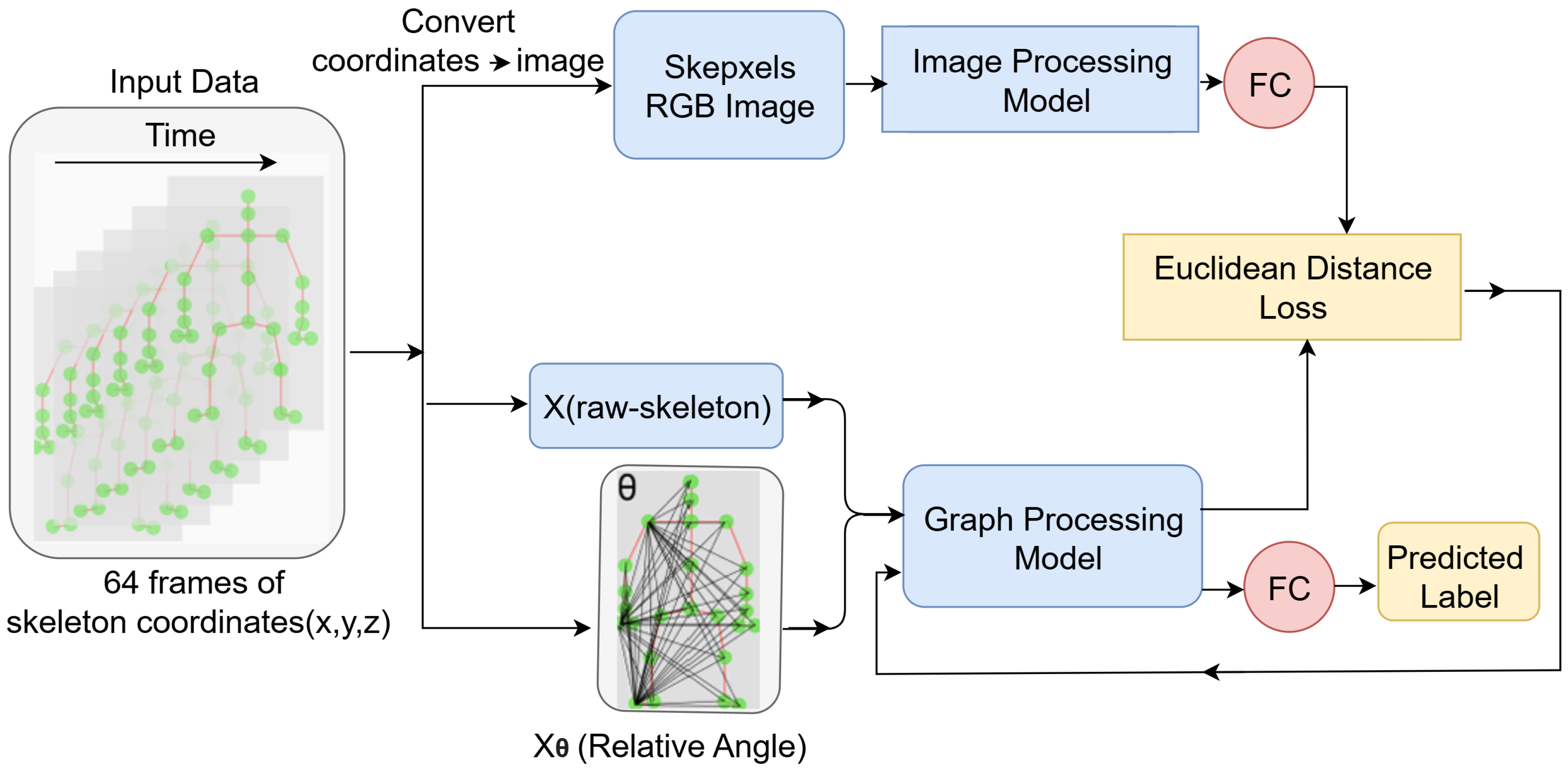
2. Proposed Methodology

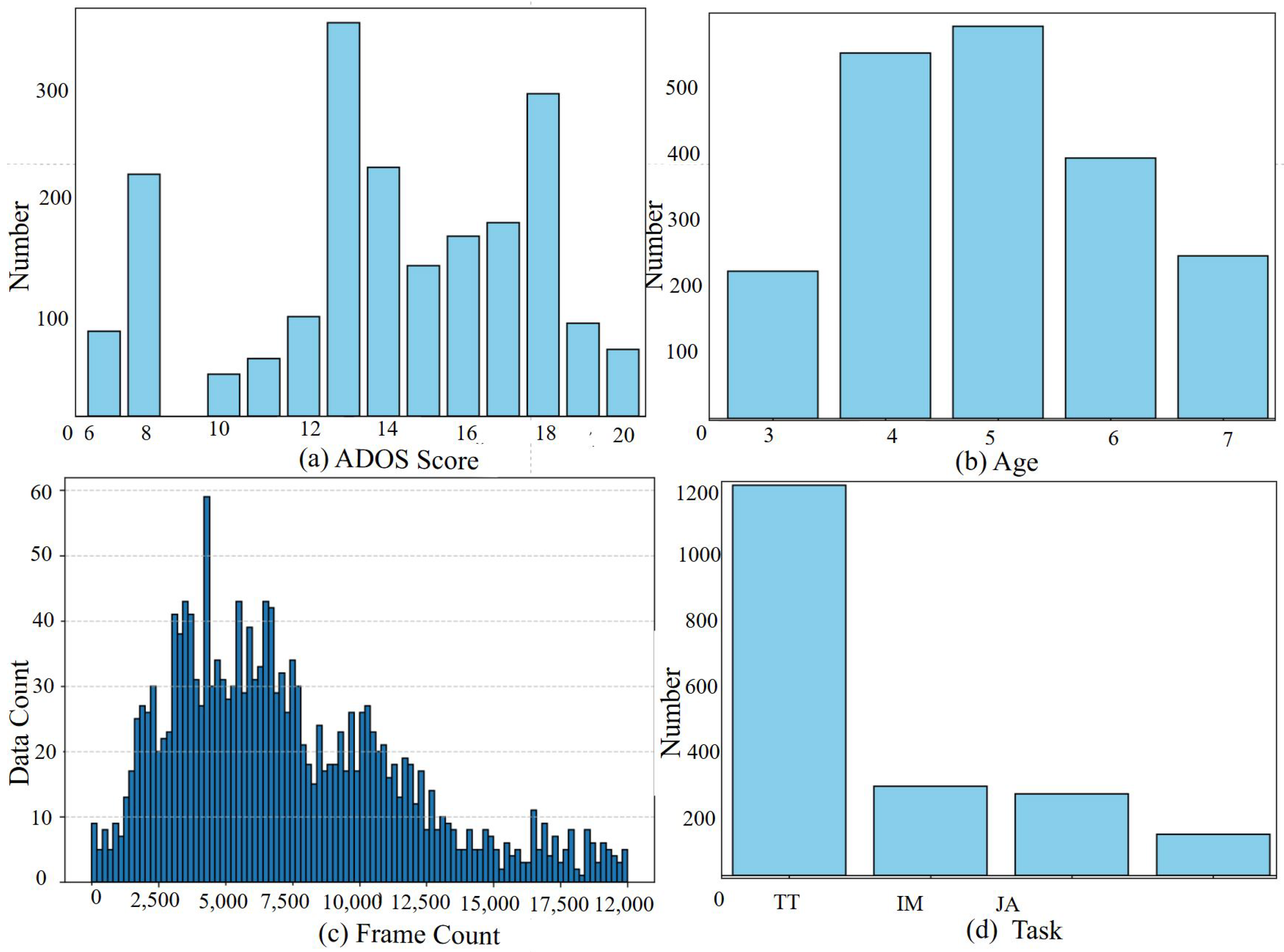
In this study, we propose an optimised dual-stream architecture for ASD detection and severity assessment, focusing on the extraction of comprehensive spatial and temporal features from skeleton-based video data. The architecture is inspired by the design presented in Sania et al. (2023) [10], but with key modifications to enhance its performance. A diagram of the proposed architecture is shown in Figure 1.

2.1. Dataset

We utilised two datasets for model evaluation. The first is the Gait Fullbody Dataset [16], and the second is the DREAM dataset [17]. The distribution of this dataset is demonstrated in Figure 2. Both are public datasets that record the body movement information of children with ASD. Our research aims to develop a model that evaluates ASD based solely on body movements, without relying on verbal communication. This approach is intended to contribute to early detection by enabling diagnosis even at stages where children have not yet developed speech abilities. Both datasets use Kinect, providing skeletal coordinate data. This is a crucial aspect for ensuring anonymity, which becomes even more important in practical applications. While ASD can also be evaluated based on facial expressions, skeletal data do not include facial information. Therefore, the model’s results can be interpreted as being derived purely from body movements. Since there are several differences between these two datasets, they will be introduced in this section. A particularly significant difference is that the Gait Fullbody Dataset uses Kinect v2, while the DREAM dataset uses Kinect v1, resulting in a difference in the number of joints recorded. To address this difference, we applied the same preprocessing method described in [10]. The preprocessing steps are explained in the following sections.

2.1.1. Gait Fullbody Dataset

The Gait Fullbody Dataset, created by Al-Jubouri et al. [9], was collected to analyse the gait and full-body movement characteristics of children with ASD and typically developing children. The dataset includes a total of 100 participants, consisting of 50 children with ASD and 50 typically developing children, with an age range of 4 to 12 years. Additionally, the dataset provides a separate subset for nine children with severe ASD symptoms. At the time of download, the dataset includes video data, 3D videos of plotted joint movements, and the x, y, z coordinates of the joints. However, in our study, we utilised only the joint coordinate data. The joint coordinates were captured using a Kinect v2 camera, and the dataset includes a total of 25 joint coordinates. Each participant performed 10 walking motions, and the most optimal trial was selected based on the disease and the doctor’s recommendation, resulting in a total of 100 samples. The dataset also offers an augmented version, as described in [9], where data augmentation increased the dataset size to approximately 700 samples. While the paper mentions that augmentation significantly improved model performance, we used only the raw joint coordinate data to ensure a fair comparison between models. Consequently, the number of data samples used in our study is 100. Figure 3 illustrates the 25 positions and the arrangement of skeleton joints captured by the Kinect V2.

2.1.2. DREAM Dataset

For the second dataset used in our model evaluation, we utilised the DREAM dataset [17]. The participants in this dataset are children aged 3 to 7 years, comprising a total of 61 children. Additionally, the ages in the dataset are represented in months. The dataset includes a total of 3121 data samples. This dataset was also collected using Kinect, and it shares a common feature with the first dataset in that it records the x, y, z coordinates of the joints. However, while the Gait Fullbody Dataset uses Kinect v2, the DREAM dataset uses Kinect v1. This difference in versions is significant, as Kinect v2 detects 25 types of joints, whereas Kinect v1 detects 5 fewer joints, resulting in a total of 20 joints. Additionally, the DREAM dataset does not include joint information for the lower body, resulting in a total of 10 joints being recorded. The dataset, in JSON format, also includes non-Kinect-derived data such as eye_gaze and head_gaze, which represent the direction of eye gaze vector and head orientation vector, respectively. The difference of 5 joints due to the version discrepancy is addressed in the later section on data preprocessing, where the missing joints are supplemented. The lower body information, which is not recorded in the original dataset, is replaced with zeros. In this dataset, labels are not provided. Instead, each data sample is assigned an ADOS score by Gotham et al. [18]. The ADOS score is used to determine the severity of ASD. The severity of ASD is determined based on three variables: the ADOS score, the module, and the participant’s age, with the distribution of these variables described in [18]. To utilise these data for model evaluation, we classified the data into three categories based on [18]: NS (Non-Spectrum), ASD, and AUT (Autistic, the most severe case of autism). In the reference study [10], the dataset did not include the NS label, resulting in a two-class classification. However, in our study, we included the NS class based on the assigned ADOS scores provided in the dataset.

Figure 2 shows the various distributions in the DREAM dataset, showing the number of samples for ADOS scores, age, the number of frames, and task types across the dataset. From this graph, it can be observed that the most frequent task is TT (Turn Taking). It should be noted that there were also data samples with blank task labels. However, since we did not restrict the tasks in our study, these samples were also included for model training. Additionally, there is significant variation in the number of frames, ranging from 27 to 35,289. Due to the large number of frames, which could cause memory issues, we decided to use only 64 frames. The preprocessing method will be described in the pre-processing section. The choice of 64 frames is considered appropriate, as this aligns with the conditions used in [10].

2.2. Dataset Preprocessing

We conducted experiments using two datasets: Gait Fullbody and DREAM, summarised in

Table 2. Dataset description used in the study.

Feature	Gait Fullbody Dataset	DREAM Dataset
Number of Participants	100 children (50 ASD, 50 typical)	61 children
Devices Used	Microsoft Kinect v2, Samsung Note 9	Kinect v1
Data Types	3D joint places (25 keypoints)	3D joint places (10 keypoints)
Task (Action)	Walking toward the camera	3 tasks (TT, IM, and JA)

. The Gait Fullbody Dataset comprises 64 frames and 25 joints, requiring no additional preprocessing. The DREAM dataset required preprocessing to replicate the experimental conditions from Sania et al. (2023) [10]. We followed the joint completion and body orientation alignment methods described in the original study, using publicly available code. For the DREAM dataset, the skeleton coordinate data, ADOS scores, modules, age in months, start frames, and end frames were provided. We identified 165 samples where the start and end frames had discrepancies, reducing the dataset from 3121 to 2957 samples. Based on ADOS score criteria from Sania et al. (2023), 1124 samples were excluded, leaving 1833 samples for experimentation [10]. Given that the DREAM dataset has a wide range of frame counts (from 27 to 35,289 frames), we standardised the frame count to 64 for all samples. For sequences exceeding 64 frames, we applied downsampling, and, for sequences with fewer than 64 frames, we used zero-padding. This ensured uniformity and reproducibility in model training and inference. Additionally, missing joint coordinates in the DREAM dataset were imputed using zero-padding to complete the joint set to 25 joints, matching the Kinect V2 format for consistency with the Graph Convolutional Network (GCN) model.

2.2.1. Joint Imputation

The DREAM dataset was collected using the Kinect V1 sensor, which does not capture the five joints available in Kinect V2: NECK, HANDTIP_LEFT, THUMB_LEFT, HANDTIP_RIGHT, and THUMB_RIGHT. The absence of these joints may affect the representation of fine-grained hand and upper body movements, as shown in Figure 3.

In [10], the missing joint coordinates were estimated through relative calculations to match the Kinect V2 joint structure. Since the DREAM dataset provides only upper-body joint coordinates, zero-padding was applied to complete the joint set to 25 joints, ensuring consistency with the Kinect V2 format. This joint imputation and zero-padding process standardised the dataset for compatibility with the GCN model, facilitating effective learning.

2.2.2. Dataset Labeling

In this study, we adopt the classification strategy based on predicted ADOS scores, ADOS module, and age, as outlined in [10,18], with slight modifications to resolve overlapping conditions between NS and ASD classes. Specifically, for the NS class in Module 2, the original criteria included children aged 3 to 4 years with ADOS scores between 6 and 7 (inclusive). To reduce ambiguity and enhance class separation, we revised this to include only those with an ADOS score equal to 6. Likewise, for children aged 5 to 6 years, we maintained the original threshold of ADOS $score\le 6$. However, this adjustment created an overlap with the ASD class, which originally included children aged 3 to 4 years with ADOS $scores>6$ and ≤9. To address this, we modified the ASD criteria to include only children within this age group who have ADOS $scores\ge 8$ and $\le 9$, thereby improving class separability. The classification for the AUT class remains unchanged from the original reference [10].

Table 3. ADOS score table.

Label Name	Module-1		Module-2
	Age	ADOS Score	Age	ADOS Score
NS	$3\sim 6$	ADOS ≤ 10	$3\sim 4$	6 = ADOS
			$5\sim 6$	ADOS ≤ 6
ASD	$6\sim$	10 < ADOS ≤ 15	$3\sim 4$	8 ≤ ADOS ≤ 9
			$5\sim 6$	ADOS = 8
AUT	$3\sim 6$	15 ≤ ADOS	$3\sim 4$	9 < ADOS
			$5\sim 6$	8 < ADOS

shows the ADOS score information for the NS, ASD, and UT.

2.3. Stream-1: Image Recognition Model Throw Skepxel

The first stream processes Skepxels, a spatial representation of the skeleton sequence, using the ConvNeXt-Base image classification model. This stream computes aggregated embeddings and employs pairwise distance loss during training, ensuring robust feature alignment and representation. Here, ConvNeXt-Base processes an aggregated embedding of the Skepxels, which is utilised during training to compute pair-wise distance loss, ensuring effective feature representation and alignment.

2.3.1. Skepxels

Applying image models to skeleton data has shown promise due to the superior performance of image-based deep learning models. To leverage this, we adopted the “Skepxels” method [14], as used in [10], to transform skeleton coordinate data into a format suitable for image models, enabling effective learning. Skepxels are constructed from Super Pixels, where each represents a 3D joint’s coordinates. Specifically, the x, y, and z coordinates are assigned to the R, G, and B channels of a 5 × 5-pixel image. With 25 joints, the resulting Super Pixel captures the entire skeleton in one frame. By integrating temporal data (concatenating 64 frames), a single Skepxels image is created and resized to 224 × 224 for compatibility with CNNs and Vision Transformers (ViTs). This transformation allows the image model to exploit its strengths, addressing the limitations of direct graph data input. While [14] primarily optimised Skepxels for CNNs, it also suggested that attention-based models might further enhance performance. In this study, we extended the original approach by conducting an ablation study, replacing the ViT-B model from [10] with a range of image models. These models were selected based on computational efficiency, ensuring comparable or lower complexity than ViT-B, to focus on meaningful advancements rather than merely increasing resource demands.

2.3.2. ConvNeXt-Base

ConvNeXt [19] is a CNN model inspired by advancements in Vision Transformers (ViT) [20] and Swin Transformers [21], while maintaining its roots in ResNet [22]. It revisits traditional convolutional architectures and incorporates modern design principles, ensuring compatibility with GPU-accelerated training and achieving competitive performance against state-of-the-art Transformer-based models. ConvNeXt introduces several enhancements over traditional CNNs, including kernel size expansion, updated normalisation techniques, and architectural optimisations. The kernel size expansion in ConvNeXt replaces the small receptive fields of ResNet with larger ones, enabling the network to capture global spatial features akin to ViT. Mathematically, the convolution operation for a kernel size $k\times k$ is expressed as Equation (1).

$$y_{i,j}=\sum _{m=0}^{k-1}\sum _{n=0}^{k-1}{w}_{m,n}·x_{i+m,j+n}+b,$$

(1)

where $y_{i,j}$ is the output feature at position $(i,j)$, $w_{m,n}$ represents the kernel weights, $x_{i+m,j+n}$ denotes the input pixel values within the kernel’s receptive field, and b is the bias term. ConvNeXt replaces Batch Normalisation (BatchNorm) with Layer Normalisation (LayerNorm) to enhance training stability, as used in ViT and Swin Transformer. LayerNorm operates along the feature dimension and normalises the input $x\in {\mathbb{R}}^{B\times H\times W\times C}$ as

$$\mathrm{LN}\left(x\right)={\displaystyle \frac{x-\mu }{\sqrt{{\sigma }^2+ϵ}}}·\gamma +\beta ,$$

(2)

where $\mu$ and ${\sigma }^2$ are the mean and variance of the input features, $\gamma$ and $\beta$ are learnable scale and shift parameters, and $ϵ$ is a small constant for numerical stability. ConvNeXt-Base processes input images through several stages, described below:

• Feature Extraction Layer: ConvNeXt-Base begins with convolutional layers to extract spatial features from the input. Given an input $X\in {\mathbb{R}}^{H\times W\times C}$, the convolutional layer produces output features Y, as described in Equation (1);
• Downsampling Layers: ConvNeXt incorporates downsampling operations to reduce the spatial resolution while preserving critical features. This is achieved using strided convolution operations, where the stride $s>1$ reduces the resolution:

  $$Y_{i,j}=\sum _{m=0}^{k-1}\sum _{n=0}^{k-1}{w}_{m,n}·x_{i+s·m,j+s·n}+b,$$

  (3)

  where s is the stride;
• Depthwise Convolution and LayerNorm: The model applies depthwise convolutions, followed by LayerNorm (Equation (2)), to improve efficiency and training stability;
• Fully Connected (FC) Layer: The final stage involves flattening the features and passing them through a fully connected layer for dimensionality reduction and final representation. If the extracted features are $f\in {\mathbb{R}}^N$, the FC operation is

  $$z=f·W+b,$$

  (4)

  where W is the weight matrix and b is the bias vector;
• ReLU Activation: Non-linearities are introduced using the ReLU activation function, defined as

  $$\mathrm{ReLU}\left(z\right)=max(0,z).$$

  (5)

ConvNeXt-Base provides various configurations, including Base, Large, Small, and Tiny versions. For this study, we selected ConvNeXt-Base to ensure computational comparability with the ViT-B model used in the original research. The architecture demonstrates superior performance by combining these innovations, achieving state-of-the-art results on benchmarks like ImageNet. In our dual-stream architecture, ConvNeXt-Base efficiently processes Skepxels, extracting global spatial embeddings and contributing to robust ASD detection.

2.4. Stream-2: Graph CNN Throw Relative Angle Information

The second stream embeds a normalized angular feature matrix, ${\left[{∥x∥}_{{\displaystyle \frac{T}{2}}}\right]}^{\theta }$, where ${∥x∥}_{{\displaystyle \frac{T}{2}}}$ denotes temporal normalization over the first half of the sequence, and the superscript $\theta$ indicates the transformation into angular features. into the input skeleton sequence. These enriched inputs are processed by MSG3D, combining GCN for spatial relationship modeling and TCN for capturing temporal dynamics.

• Angular Matrix

The angular feature matrix, represented as ${\left[{∥x∥}_{{\displaystyle \frac{T}{2}}}\right]}^{\theta }$, is a critical component for enriching the input skeleton sequence with meaningful spatial–temporal relationships. Here, ${∥x∥}_{{\displaystyle \frac{T}{2}}}$ denotes the normalised joint positions, and $\theta$ represents the relative angular relationships between joint pairs. The normalisation of the skeleton coordinates ensures consistency across variations in scale and posture, allowing the model to focus on intrinsic movement patterns. The angular feature matrix captures the angular relationships between all joints in the skeleton sequence. These angular features are computed by measuring the angles between pairs of joints, forming a comprehensive $N\times N$ matrix, where N is the number of joints (e.g., $N=25$ for datasets with 25 joints). This matrix provides additional geometric context to the skeleton data, encoding subtle posture dynamics and asymmetry that are critical for recognising ASD.

• Angle Embedding

In this study, the graph model is trained using skeleton coordinate data with angle embedding, as introduced in [10]. The effectiveness of this method for ASD detection was demonstrated in [10]. It is suggested that children with ASD tend to exhibit distinctive slanted postures and asymmetry, and learning these features can contribute to improving detection accuracy. The angle embedding process integrates the angular features into the original skeleton input, enhancing the input representation for the model. This process is mathematically defined as

$$X_{\mathrm{norm}}=\sqrt{\sum _{t=1}^T{\parallel X\parallel }^2},\overline{X}={\displaystyle \frac{X}{X_{\mathrm{norm}}}},X_{i,j}^{\theta }={\overline{X}}_i·{\overline{X}}_j$$

(6)

Here, X represents the input skeleton coordinate data, and $X_{\mathrm{norm}}$ is the normalisation factor computed over all frames T in the sequence, ensuring consistency across samples. $\overline{X}$ is the normalised skeleton coordinate data, obtained by dividing the original coordinates X by $X_{\mathrm{norm}}$; $X_{i,j}^{\theta }$ computes the cosine similarity between the normalised vectors of joint i and joint j, capturing the relative angular relationship between them. First, the input skeleton data are normalised to obtain $X_{\mathrm{norm}}$. Using the normalised coordinates, the angles between each pair of joints are calculated, resulting in a 25 × 25 matrix that captures the angular features between all joints (since there are 25 joints). Finally, the input data are multiplied by the joint angle matrix to create input data that incorporates angular information in a form suitable for learning by the graph model. The graph algorithm introduced in Section 2.4 is then used to train the model with these generated data. This process results in an angular feature matrix of size $N\times N$ (e.g., $25\times 25$), where each element encodes the angular relationship between a pair of joints. The angular feature matrix is then combined with the normalised input skeleton data to create an enriched input representation. This enhanced input is subsequently processed by the MSG3D model, which utilises GCN for spatial feature extraction and TCN for temporal feature extraction.

The angular features effectively capture slanted postures and asymmetries often exhibited by children with ASD. The angular matrix encodes critical geometric relationships, enabling the model to understand the spatial dynamics of movement better. This enriched input representation, combined with the dual-stream architecture, provides a robust framework for ASD detection and severity assessment.

• Graph-CNN on the Relative Angle Features

The Graph Convolutional Network (GCN) processes the angular embedding output to extract hierarchical spatial–temporal features critical for ASD detection. This section details the GCN’s functionality, leveraging the enriched input representation provided by the angular embedding. The Graph Convolutional Network (GCN) [23] is a neural network designed to process graph-structured data. While CNNs are designed to process grid-like data such as images, GCNs were proposed to handle graph data composed of nodes and edges. The human skeleton is represented as a graph $G=(V,E)$, where $V=\{v_1,v_2,\dots ,v_N\}$ are the nodes corresponding to skeleton joints. $E=\{e_1,e_2,\dots ,e_M\}$ are the edges representing connections (bones) between joints. The graph is encoded using an adjacency matrix $A\in {\mathbb{R}}^{N\times N}$, where $A_{ij}=1$ if there is an edge between nodes i and j. To incorporate self-loops, the adjacency matrix is augmented as $\tilde{A}=A+I$, where I is the identity matrix. The node features are initialised using the angular feature matrix $X^{\theta }$, which encodes the angular relationships between joints. This matrix, combined with normalised skeleton coordinates, provides a comprehensive representation of the skeletal structure. GCN applies localised convolution operations over the graph’s nodes and their neighbors to extract spatial features. The output of a GCN layer is given by

$$X^{(l+1)}=\sigma \left({\tilde{D}}^{-{\displaystyle \frac{1}{2}}}\tilde{A}{\tilde{D}}^{-{\displaystyle \frac{1}{2}}}{X}^{\left(l\right)}{\mathrm{\Theta }}^{\left(l\right)}\right),$$

(7)

where: $\tilde{A}$ is the augmented adjacency matrix. $\tilde{D}$ is the diagonal degree matrix of $\tilde{A}$. $X^{\left(l\right)}$ is the input feature matrix at layer l, initialised with $X^{\theta }$ for the first layer. ${\mathrm{\Theta }}^{\left(l\right)}$ is the learnable weight matrix for layer l. $\sigma$ is the activation function, typically ReLU. Research on processing joint data with GCNs has been active, such as the proposal of ST-GCN [24,25], a model for processing time-series joint data. The data we handle in this study are skeleton data, which can be processed as graph data composed of bones (edges) and joints (nodes). MSG3D (Multi-Scale Graph 3D Convolutional Network) [26] is a powerful model designed to analyse complex movements in skeleton data, such as human actions. It addresses common problems in traditional Graph Convolutional Network (GCN) models. One major problem is that traditional GCNs focus too much on nearby nodes and fail to consider information from distant nodes. Another issue is that spatial (joint connections) and temporal (time-based changes) information are processed separately, making it hard to capture the full relationship between these dimensions. To solve these problems, MSG3D introduces two key methods. First, Disentangled Multi-Scale Aggregation (MS) reduces the overemphasis on nearby nodes by using distance-specific adjacency matrices. These matrices help the model learn meaningful information from both nearby and distant nodes. Second, the Unified Spatial–Temporal Graph Convolution (G3D) combines spatial and temporal data effectively. Using skip connections, it links joints across different time frames, helping the model learn how joint movements change over time. These features make MSG3D highly effective for tasks like ASD detection, where it is important to understand both the spatial and temporal movement patterns.

2.5. Model Integration and Training

The outputs from both streams (image- and graph-based models) are combined using pairwise Euclidean distance loss to ensure consistent feature representation. This loss function ensures effective alignment between spatial and temporal features for optimal ASD detection. The dual-stream architecture proposed in this study leverages both image classification (ConvNeXt-Base) and graph convolutional networks (MSG3D) to enhance ASD detection by capturing both spatial and temporal dynamics. By integrating angular features, this model effectively addresses the complexities of movement patterns associated with ASD, paving the way for more accurate and interpretable ASD detection systems.

3. Experimental Result

In the study, we evaluated the proposed model with two benchmark video datasets. First, we extracted the skeleton point from the sequence of frames using pose estimation systems. In this section, we describe the environmental setup, ablation study, performance evaluation, and state-of-the-art comparison for both datasets. In the study, we use the Euclidean distance loss on training and test individual streams separately.

3.1. Environmental Setting

The experiments were conducted on the DREAM dataset using a controlled Python-based environment. Each image model was trained for 30 epochs initially, employing 10-fold cross-validation, with the process repeated three times per model to ensure performance consistency. The dataset, consisting of 1833 samples, was split into 1650 samples for training and 183 samples for testing per fold. To further improve model performance, the number of epochs was extended to 100 after observing the learning curves during preliminary trials, which provided insights into the convergence behaviour of the models. The experimental setup was developed using Python (version 3.10). The experimental setup was developed using Python (version 3.10). PyTorch (version 2.5.1.post302), Torchvision (version 0.20.1a0+9f8010e), NumPy (version 1.26.4), scikit-learn (version 1.5.1), SciPy (version 1.13.1), Seaborn (version 0.13.2), Pandas (version 2.2.2), OpenCV (opencv-python version 4.10.0), and OpenCV-Python-Headless (version 4.10.0). An NVIDIA GeForce RTX 3090 GPU with 48 GB of RAM and Ubuntu OS was utilised, ensuring efficient parallel processing for deep learning tasks. The models were trained using a stochastic gradient descent (SGD) optimiser with a learning rate of 0.001 and a batch size of 12. For each of the five image recognition models tested, the results were collected from a complete cycle of 10-fold cross-validation to ensure reliable performance comparisons across different architectures. This standardised experimental design allowed for a robust evaluation and the reproducibility of the results.

3.2. Training and Testing Configuration

We trained the model with the Euclidean distance loss for both streams and tested each stream separately, even though the model was trained to leverage the combined representations. The Euclidean distance loss minimises the distance between the Skepxel embedding, which captures spatiotemporal features, and the GCN embedding, which models structural joint relationships. This alignment helps both streams (Stream-1 and Stream-2) to learn complementary features, improving overall representation for autism detection. By promoting co-learning, the loss enhances the interaction between spatial and temporal features, enabling the model to better combine these elements, thus improving the final decision-making process. In addition, the Euclidean loss encourages the streams to learn meaningful and aligned feature representations, resulting in more accurate predictions during testing. It also aids in optimisation by providing gradients that account for learning in both streams, allowing the model to understand how changes in one stream affect the other. This holistic learning process helps to improve convergence and the model’s ability to effectively integrate both types of data.

3.2.1. Reason for Individual Streams Tests

After training the model with the Euclidean distance loss, a reviewer might question the benefit of testing the individual streams (Stream-1 and Stream-2) separately, even though the model was trained to leverage the combined representations. The following points justify the significance of this approach:

Understanding Individual Stream Contributions

Testing the streams individually—Stream-1 using Skepxel with ViT and Stream-2 using Angle+GCN—helps to understand how each stream contributes to the overall performance. By analysing their separate results, we can enable an evaluation of whether one stream is significantly more effective in identifying autism or predicting severity. For instance, if Stream-2 (Angle+GCN) outperforms Stream-1, this indicates that the structural joint relationships captured by GCN may hold greater relevance for autism detection. Certain streams may be more sensitive to specific autism-related features—e.g., gestures, fine motor movements, or postural patterns—allowing us to understand which modality captures different behavioural cues more effectively.

Performance Comparison

Comparing each individual stream’s performance with that of the combined model provides insights into the true value of the two-stream architecture. If the combined model significantly outperforms each individual stream, this confirms the synergistic benefit of fusing spatial and structural information.

Better Interpretability and Debugging

Individual stream analysis aids in understanding the model’s behaviour and interpretability. This allows the identification of which features contribute more effectively to the diagnosis and prediction tasks. Moreover, this diagnostic approach can help to identify underperforming components. For example, if the Skepxel stream is less effective at capturing subtle features, targeted improvements can be planned.

Insights for Future Improvements

Evaluating stream-wise performance can guide model enhancements. If Stream-1 (Skepxel with ViT) yields suboptimal results, it may indicate the need for better temporal modeling or spatiotemporal encoding techniques. If Stream-2 (Angle+GCN) shows limited performance, improvements in joint angle representation or the adoption of more expressive GCN architectures may be necessary.

3.2.2. Euclidean Distance Loss and Its Benefits for Individual Stream Testing

The inclusion of Euclidean distance loss during training encourages stronger alignment between the embeddings generated by both streams. As a result, even when testing the individual streams separately, the model benefits from the prior co-learning phase, during which both streams were optimised to learn complementary features. This leads to the following benefits.

Enhanced Feature Representation

The Euclidean loss aligns the feature spaces of both streams, resulting in embeddings that capture useful and complementary aspects of autism-related gestures and movements. This alignment helps to improve each stream’s standalone performance at test time, even though the training emphasised combined learning.

Informed Individual Stream Evaluation

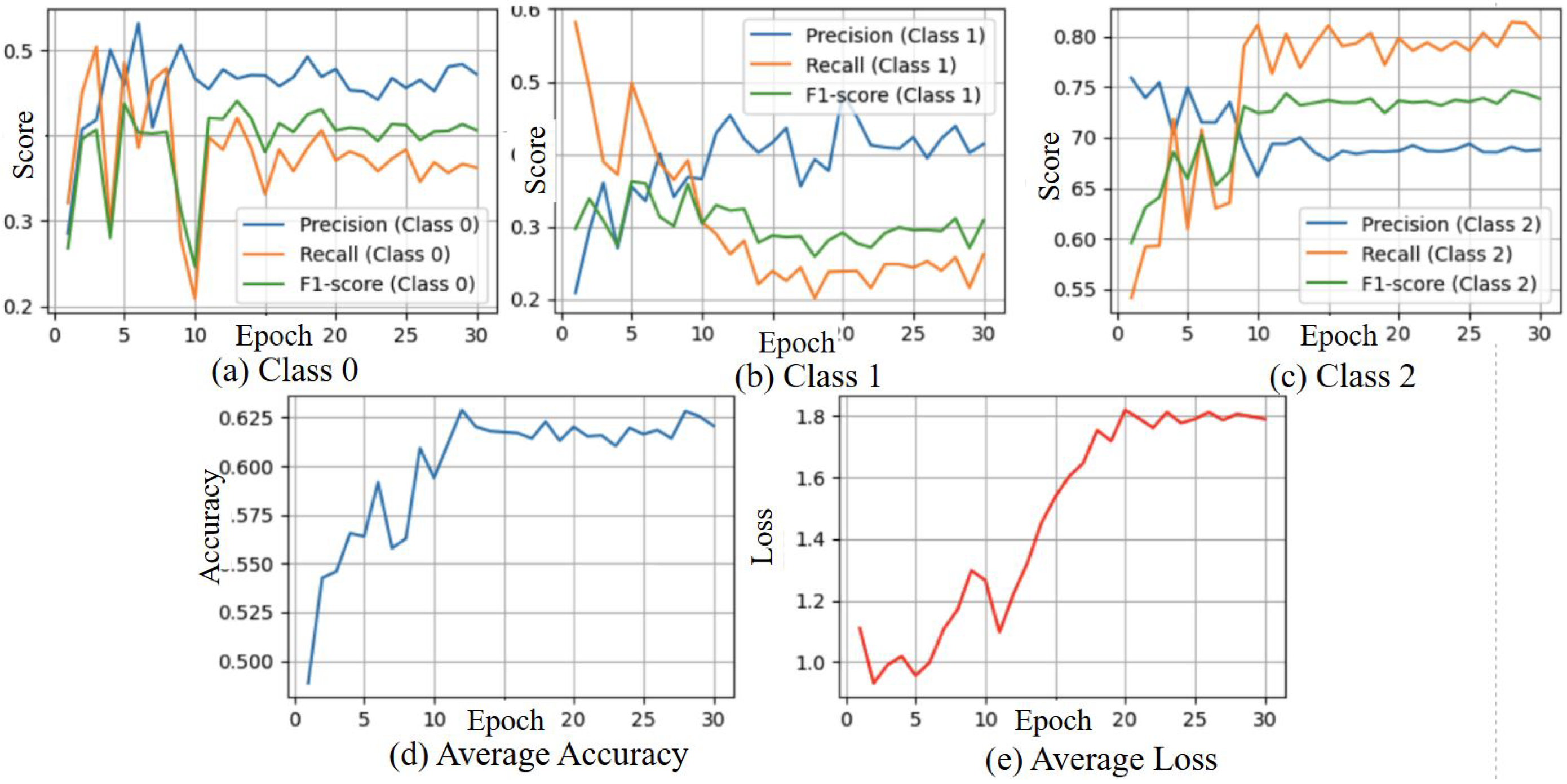
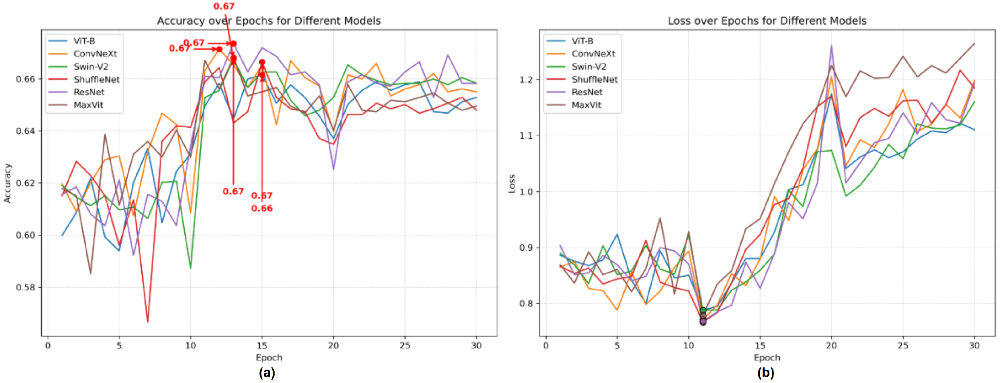
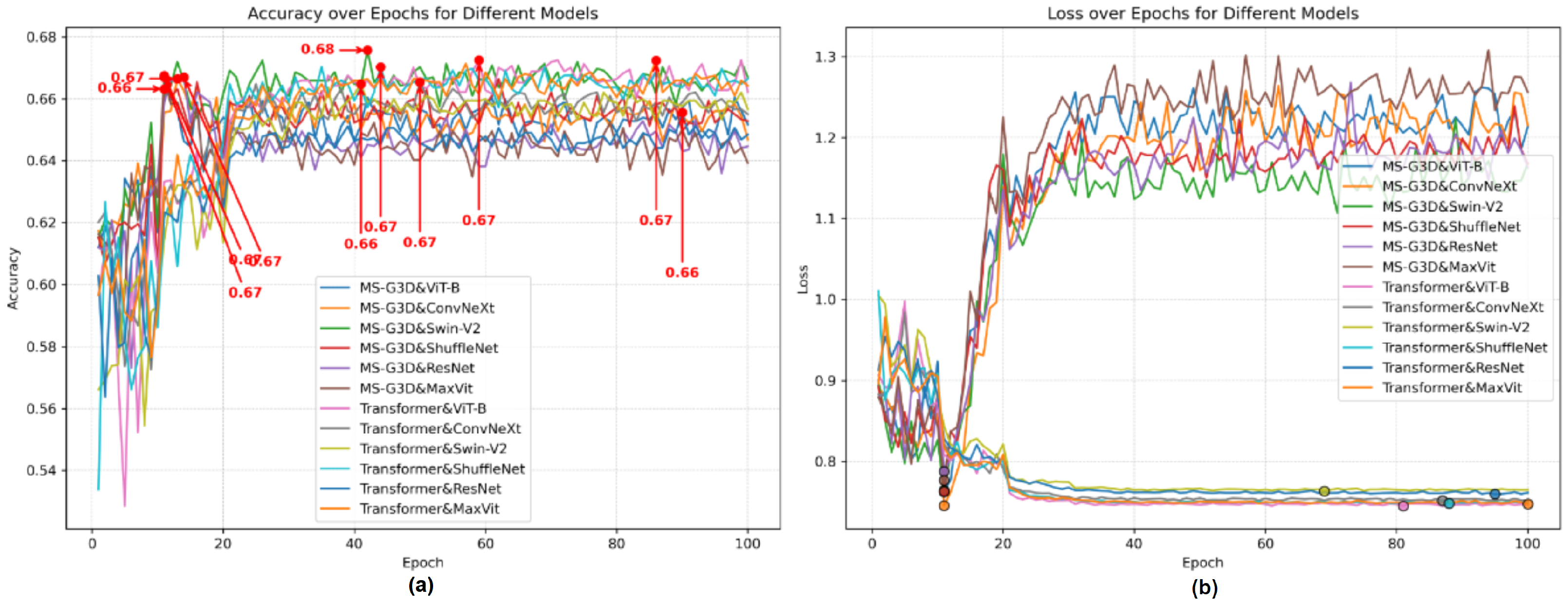
Although the combined two-stream model is expected to yield the highest accuracy, analysing the individual streams post-training helps us to understand the specific contributions of each modality (spatiotemporal via Skepxel+ViT and structural via Angle+GCN). This helps to reveal how well the Euclidean loss facilitated knowledge transfer between the streams. These insights validate the impact of the Euclidean distance loss not only on joint learning but also on each stream’s standalone robustness.

3.3. Ablation Study

In this section, we describe the tuning of the model shown in Figure 1, where we optimised the model and compared the performance results. Specifically, we explain the method of replacing the image model ViT-B used in [10] with five models selected in this study. The replacement process was straightforward: the substituted models received Skepxels as input, and their output features were incorporated into the Euclidean loss calculation. Apart from replacing the image model, all other experimental conditions remained unchanged. Additionally, for comparison purposes, the original ViT-B model from the referenced study was also executed in our environment using the same procedure. Therefore, the obtained results are consistent and reflect a unified experimental setup.

3.3.1. Ablation Study with Gait Fullbody Dataset

In the Gait Fullbody Dataset, each image model was trained for 30 epochs using a 10-fold cross-validation setup, and this experiment was repeated five times for each model to calculate the average performance. During this process, the GitHub code provided in [10] was used. However, it is important to note that the option cluster_distance_loss must be set to True to enable the use of Skepxels. Since the original dataset contains 100 samples, the 10-fold cross-validation splits the data into 90 samples for training and 10 samples for testing in each learning. The averaged results were calculated from a total of 50 training runs (10 folds × 5 run). Figure 4 shows the learning graph for the ViT-B model over 30 epochs. The loss drops sharply around the 13th epoch, indicating that the binary classification task is progressing effectively.

3.3.2. Ablation Study with DREAM Dataset

In the DREAM dataset, each image model was trained for 30 epochs using 10-fold cross-validation, and the experiment was repeated three times for each model to calculate the average performance. While the Gait Fullbody Dataset was tested five times, the DREAM dataset was limited to three runs due to its large size and computational resource limitations. With 1833 samples in the dataset, the 10-fold cross-validation split resulted in 1650 training samples and 183 test samples per fold. Figure 5 shows the learning curve for the ViT-B model trained over 30 epochs with 10-fold cross-validation. The loss decreases until around the 13th epoch, but then continuously increases, with no further improvement in maximum accuracy. This trend indicates overfitting in the DREAM dataset. The accuracy at this point was 69.34%.

3.3.3. Ablation Study with Data Augmentation of DREAM Dataset

In this study, data augmentation was experimentally applied as one approach to address the issue of overfitting. In the DREAM dataset, there was a significant class imbalance among labels, which was addressed through data augmentation to observe its impact on model performance. Specifically, the distribution of the training data was as follows: NS—432, ASD—195, and AUT—1021, with the AUT class being considerably larger than the others. To mitigate this imbalance, slight rotations and scale changes were applied to the NS and ASD data, resulting in a 2× increase for NS and a 4× increase for ASD. The results of training with the augmented data are shown in Figure 6. Compared to training without data augmentation, the learning curve indicates that overfitting occurred even earlier, and the accuracy dropped to 65.28%. Based on these findings, the results presented in the ablation study focus on experiments without data augmentation.

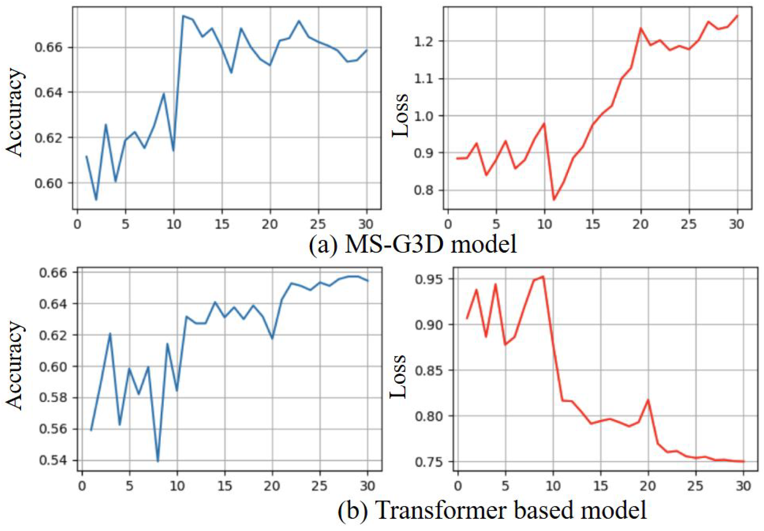
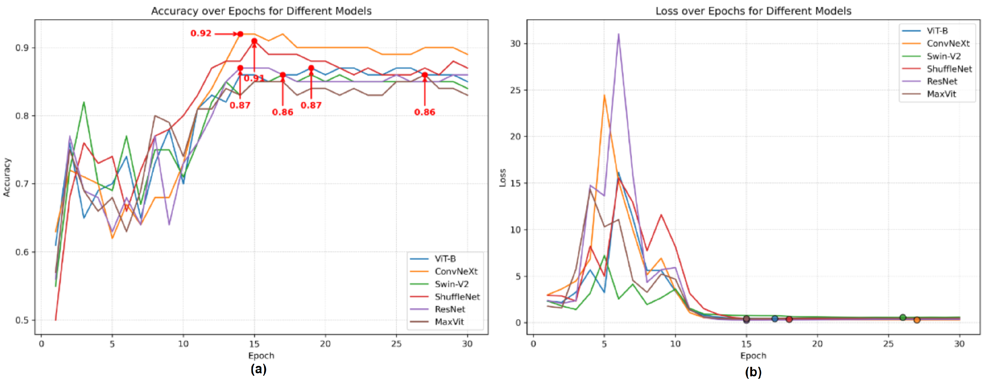
3.3.4. Ablation Study of Skeleton Coordinate Recognition Models

In this section, we investigate the training process and accuracy by replacing the GCN model MSG3D, used in [10], with a Transformer-based model [27]. This experiment allows us to not only evaluate the performance of image recognition models but also to discuss the comparison between GCN models and Transformer-based models for skeleton coordinates data processing. The focus of this experiment is on the DREAM dataset, where overfitting occurred rapidly in the above Section 3.3.2. By modifying the graph model, we aim to explore how different coordinate processing architectures impact learning in this challenging dataset. The results of the model replacement were collected by performing a 1-set of 10-fold cross-validation experiment for each of the five image recognition models. Regarding the number of epochs, we decided to extend the training to 100 epochs based on the analysis of the learning curves obtained after initial experiments. The reasoning behind this decision is explained in detail. Figure 7 shows the results of experiments conducted for 30 epochs using the Transformer-based model.

The average accuracy did not surpass that of MSG3D (69.34%) and resulted in 67.14%. However, upon examining the learning curve of the loss, it can be observed that the loss gradually decreases as the number of epochs increases. As long as this decreasing trend continues, it is reasonable to assume that additional training could further improve accuracy. Figure 8 shows a comparison between the loss curve of MSG3D and that of the Transformer-based model, highlighting the differences in learning behaviour between the two models.

In contrast to MSG3D, which rapidly reduces its loss and reaches its peak accuracy at an early epoch, the Transformer-based model continues to improve its accuracy progressively with each additional epoch. Since the Transformer-based model did not exhibit the overfitting issue observed in MSG3D and was able to continue learning effectively, it was decided to increase the number of epochs for the graph recognition process from 30 to 100.

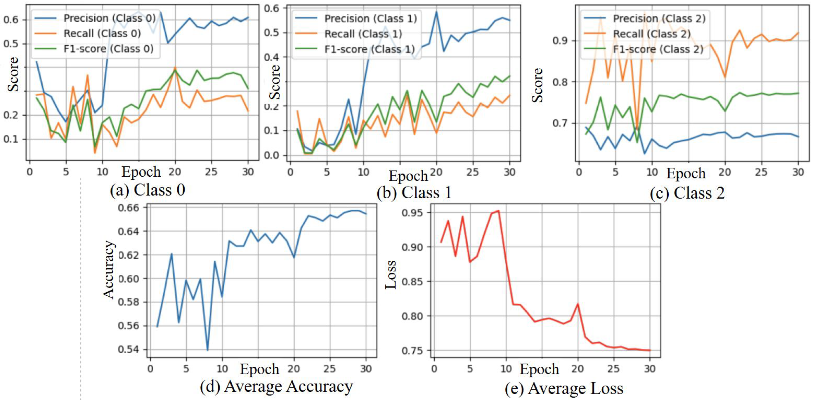
3.4. Result from Stream 1 Ske-Conv Model with Loss from Both Streams

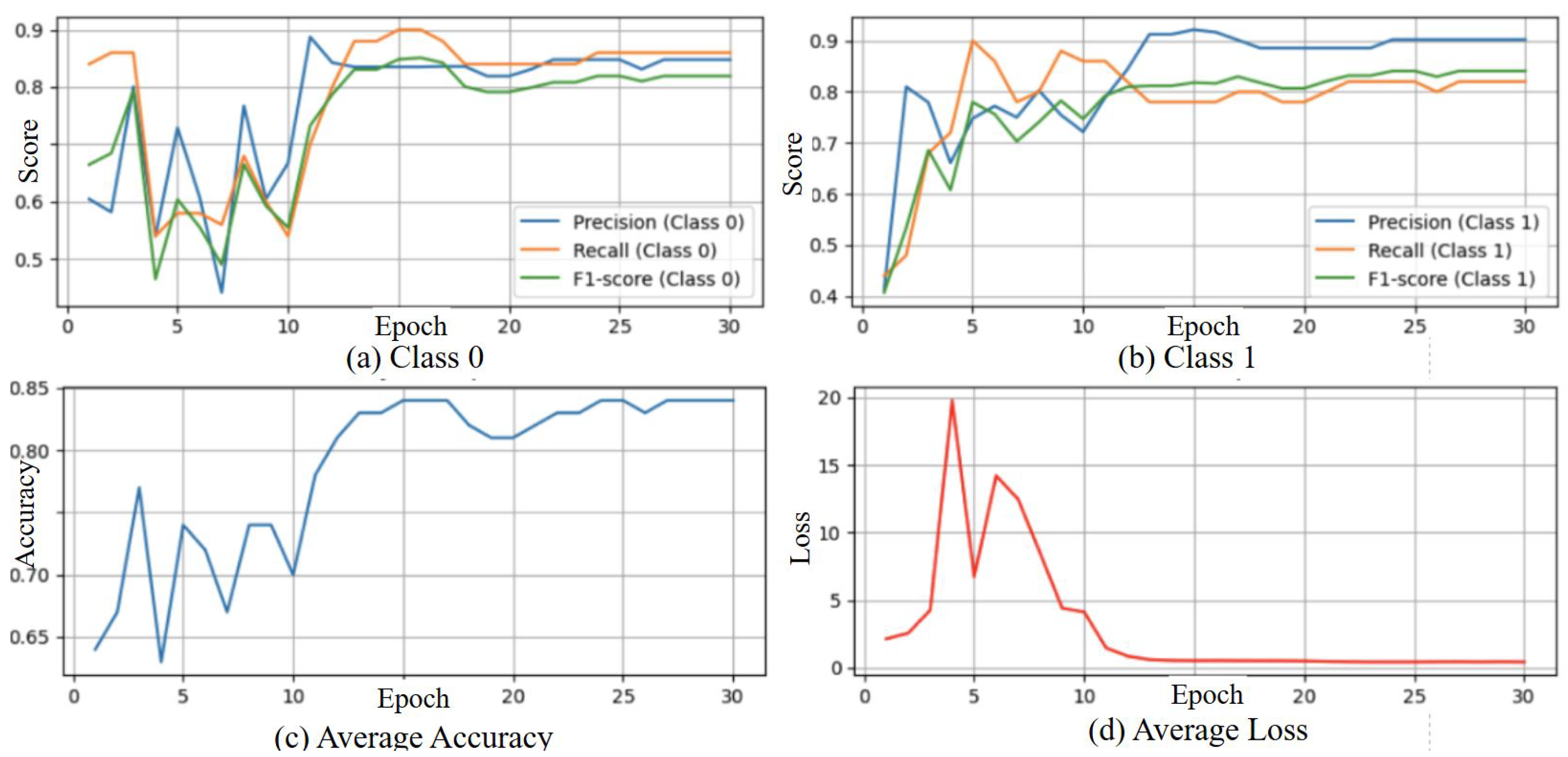
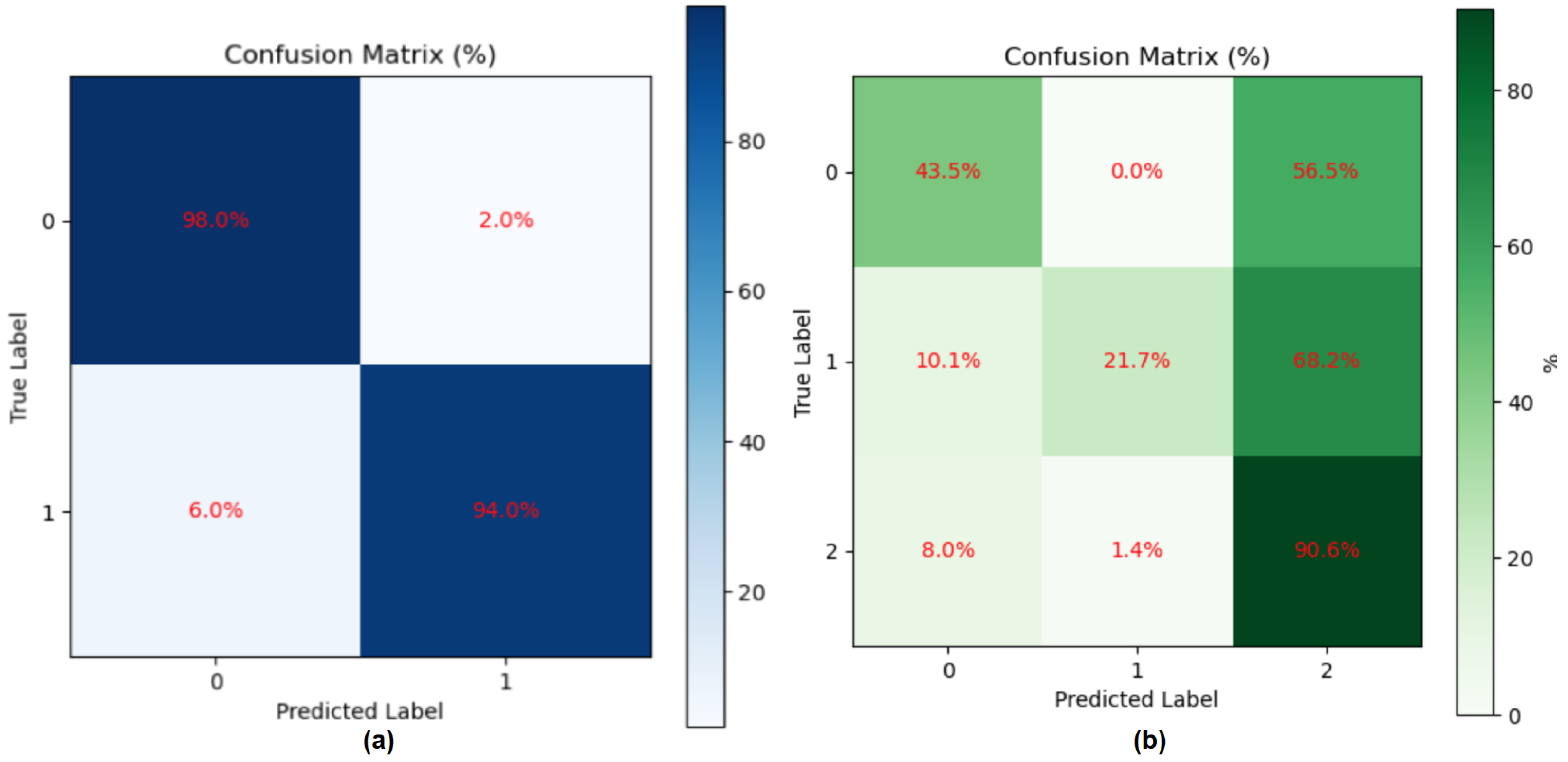
3.4.1. Result of Gait Fullbody Dataset Experiment

The experiments on the Gait Fullbody Dataset were aggregated for each of the six image recognition models. The average accuracy over five runs, along with the highest accuracy, lowest accuracy, and standard deviation, are presented in

Table 4. Image recognition model performance on Gait Fullbody Dataset.

ModelName	AveAcc (%)	MaxAcc (%)	MinAcc (%)	SD	Architecture Type
ViT-B(ref)	94.8	96.0	94.0	0.83	Transformer
ConvNeXt-Base	95.0	96.0	94.0	1.00	CNN
Swin-V2-B	93.2	94.0	92.0	0.83	Transformer
ShuffleNetV2-X2	95.4	97.0	94.0	1.14	CNN
ResNet-152	94.0	95.0	93.0	0.71	CNN
MaxViT-T	95.4	97.0	93.0	1.82	CNN + Transformer

.

In the experimental results on the Gait Fullbody Dataset, ShuffleNet and MaxViT achieved the highest accuracy of 95.4%, followed by ConvNeXt with 95.0%. Additionally, by examining the standard deviation (SD), it was observed that ShuffleNet demonstrated more stable performance compared to MaxViT. Figure 9 illustrates the averaged accuracy and loss per epoch for all six models. Since this graph represents averaged values, the epochs at which the highest accuracy is achieved do not necessarily align across models. Therefore, it is important to note that there may be differences between the results shown in the table and the peak accuracy points in the graph.

For all models, the loss trends during training exhibit similar patterns. Around epoch 5, the loss increases sharply; however, after surpassing epoch 10, the models continue to achieve high-accuracy learning. By the time that they reach epoch 20, the learning process reaches its limit. The results obtained using the Gait Fullbody Dataset demonstrated high accuracy. In the comparison study from [10], when the same model was run with randomly selected data, the reported accuracy was a maximum of 96.67% and an average of 92.33%. In contrast, our experimental environment yielded a maximum accuracy of 96.0%, which is comparable, but the average accuracy of 94.8% was notably higher. When comparing the average accuracy of the replaced image models and ViT-B, models such as ConvNeXt-Base, ShuffleNetV2-X2, and MaxViT-T outperformed ViT-B in terms of average accuracy. The highest accuracy was achieved by both MaxViT-T and ShuffleNetV2-X2, each recording 95.4%. As shown in the image model comparison in Table 4, ShuffleNet has significantly fewer parameters and lower computational complexity compared to the other models. Despite being a lightweight model, ShuffleNet achieved high accuracy, making it a good model among the selected image models. Additionally, the average 10-fold accuracy and loss learning curves in Figure 9 indicate that ConvNeXt consistently maintained a higher position in the later epochs. This can be attributed to its relatively low standard deviation and its higher recorded accuracy of 95.0% compared to ViT-B. These results suggest that ConvNeXt delivers stable performance with minimal influence from random factors. Moreover, since its accuracy does not significantly drop even after more epochs, further improvements in preprocessing or data augmentation could potentially enhance its learning capabilities.

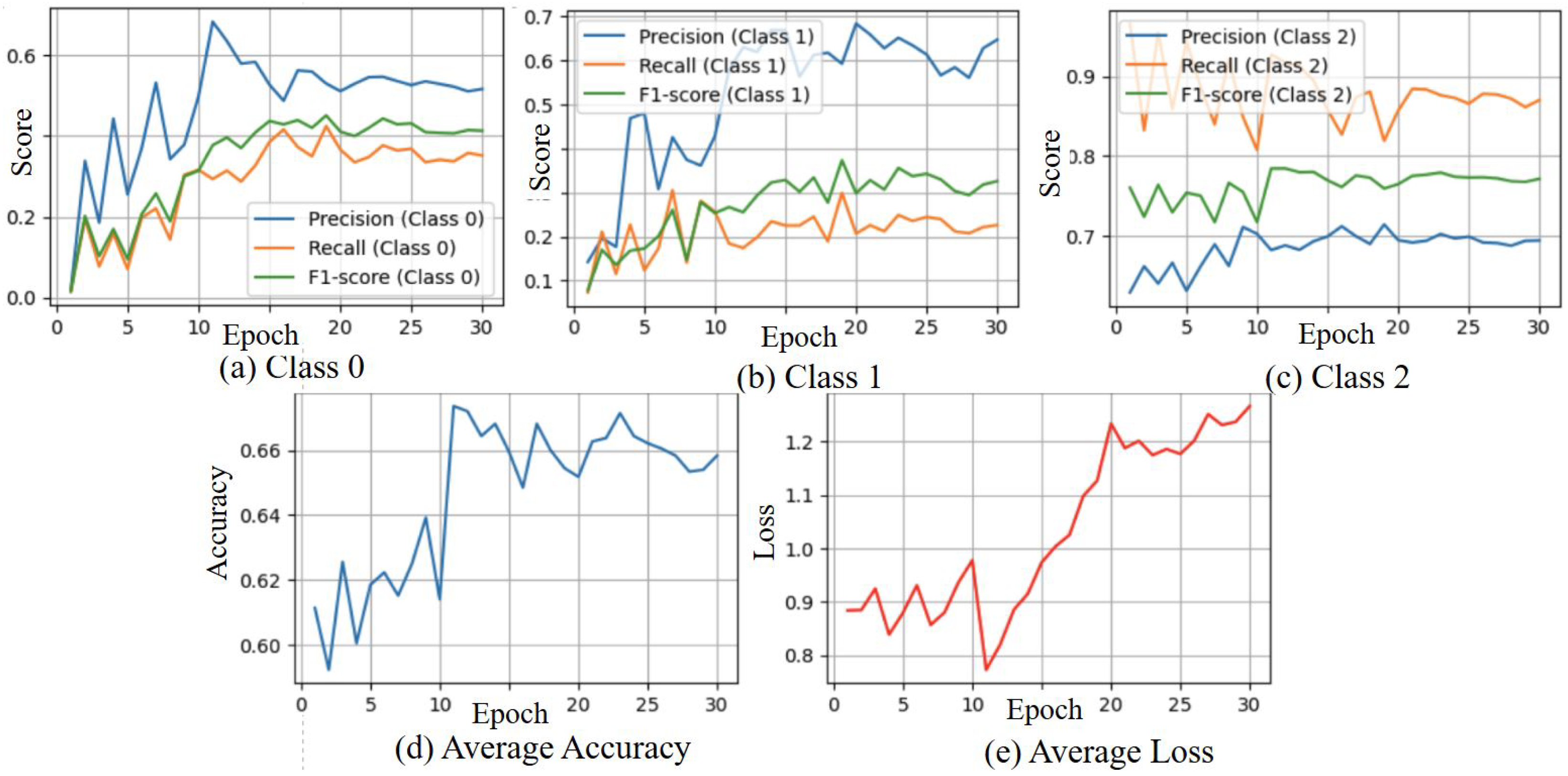
3.4.2. Results of DREAM Dataset Experiment

In the experiment using the DREAM dataset, the average accuracy, max accuracy, min accuracy, and standard deviation for each of the six models, calculated over three runs, are presented in

Table 5. Image recognition model performance on DREAM dataset.

ModelName	AveAcc (%)	MaxAcc (%)	MinAcc (%)	SD	Architecture Type
ViT-B(ref)	69.34	69.87	68.61	0.65	Transformer
ConvNeXt-Base	70.19	70.80	69.43	0.69	CNN
Swin-V2-B	69.28	69.75	68.39	0.77	Transformer
ShuffleNetV2-X2	68.96	69.54	68.45	0.54	CNN
ResNet-152	69.24	69.43	69.15	0.15	CNN
MaxViT-T	68.92	69.81	67.90	0.96	Transformer

below.

Reviewing the experimental results of the DREAM dataset, ConvNeXt-Base achieved the highest accuracy at 70.19%, followed by ViT-B with 69.34%. Other models showed minimal differences in performance. Notably, ResNet exhibited a significantly lower standard deviation (SD) across the three runs compared to the other models, indicating more consistent performance.

The Figure 10 presents the averaged accuracy and loss curves across epochs for all six models.

Focusing on the accuracy graph, it can be observed that, up to around the 10th epoch, the performance of each model’s learning is at a high speed. However, after this point, a gradual decline is seen across all models. Additionally, the loss graph shows a distinctive pattern. All models reach their lowest loss at the 11th epoch, followed by a sharp increase in loss.

When comparing the results of the DREAM dataset with those reported in the reference study [10] using the same model, our experiment showed an average accuracy of 69.34% for ViT-B, when the reference study reported a higher accuracy of 78.6%. The difference in accuracy for the same model may be attributed to different methods in the preprocessing steps that were not explicitly detailed in the reference paper. Additionally, the reference study conducted classification tasks were separated individual participant actions, which likely contributed to achieving higher accuracy. In contrast, we treated all actions as a single dataset, potentially increasing classification complexity. However, the fact that accuracy did not drastically drop despite mixing different tasks suggests that the model may have successfully learned common ASD-related features across various actions. Due to the large scale of the DREAM dataset, the differences in accuracy across models and experimental repetitions were minimal. Nonetheless, ConvNeXt achieved the highest accuracy at 70.19%, followed by ViT-B at 69.34%, with a gap of only 0.85%. This indicates that ConvNeXt was particularly well-suited for this dataset. However, across all models, the loss rapidly increased, which strongly suggests the occurrence of overfitting. The model replacement strategy for image recognition models did not resolve this issue, leading to the conclusion that only a limited amount of training was effective for the DREAM dataset.

3.5. Results from Stream 2 Angle Skeleton-Based Model with Loss from Both Streams

In this section, we show results of experiments using the skeleton classification models for the Dream dataset, specifically comparing the performance of the MSG3D model used in [10] with the Transformer-based model that we prepared for comparison. This experiment also summarises the results obtained by replacing the six different image models. Unlike the ablation study on image classification models, which was conducted over 30 epochs, this section employed 100 epochs. This decision was made because the Transformer-based model continued to improve its learning beyond 30 epochs. Each combination of the two skeleton classification models and six image classification models was executed once, and the results are presented in

Table 6. Accuracy comparison of two skeleton classification models with six image classification models for Dream dataset.

Skeleton Classification Model	Image Classification Model	Architecture Type	Accuracy (%)	Ave Acc (%)
MSG3D (GCN-based)	ViT-B (ref)	Transformer	68.94	69.39
	ConvNeXt-Base	CNN	69.26
	Swin-V2-B	Transformer	70.52
	ShuffleNetV2-X2	Lightweight CNN	69.38
	ResNet-152	CNN	69.27
	MaxViT-T	CNN + Transformer	68.99
Transformer-based [27]	ViT-B (ref)	Transformer	68.77	68.08
	ConvNeXt-Base	CNN	68.23
	Swin-V2-B	Transformer	67.62
	ShuffleNetV2-X2	Lightweight CNN	68.39
	ResNet-152	CNN	66.81
	MaxViT-T	CNN + Transformer	68.66

.

Although the experiments were conducted using 10-fold cross-validation, it is important to note that, due to computational resource limitations, we could not average the results over multiple runs. As a result, Swin-V2 achieved the highest accuracy of 70.52% with the MSG3D model, while ViT recorded the highest accuracy of 68.77% with the Transformer-based model. On the other hand, when comparing the average accuracy between the two skeleton recognition models, a significant difference was observed. MSG3D achieved an average accuracy of 69.39%, while the Transformer-based model achieved 68.08%. The learning curves for accuracy and loss over 100 epochs, generated using the logged results presented in the table, are shown in Figure 11.

The MSG3D model, similar to the results in the image model ablation study (Section 3.7), achieved its highest accuracy and lowest loss around the 11th epoch. Also, after this point, the loss increased, and this trend persisted throughout the 100 epochs. In contrast, the Transformer-based model exhibited a gradual decrease in loss over time, with the epoch at which maximum accuracy was achieved varying across different image models. Notably, the combination of MaxViT and the Transformer-based model recorded the lowest loss at the 100th epoch.

3.6. State of the Art Comparison for Gait Fullbody Dataset

Table 7. State-of-the-art comparison of the proposed model on the Gait Fullbody Dataset.

Method	Data	Subject Selection	Accuracy (%)	Precision (%)	Recall (%)	F1-Score (%)
Ahmed et al. [9]	Skeleton	Random	92.00	–	–	–
Sania et al. [10]	Skeleton	Random Average	92.33	–	–	–
Proposed (Ours)	Skeleton	Random Average	95.00	97.92	94.00	95.92

shows the state of the art comparison for the Gait Fullbody Dataset. In the experimental results on the Gait Fullbody Dataset, ShuffleNet and MaxViT achieved the highest accuracy of 95.4%, followed by ConvNeXt with 95.0%. Additionally, by examining the standard deviation (SD), it was observed that ShuffleNet demonstrated a more stable performance compared to MaxViT. Figure 12a demonstrates the confusion matrix of the proposed model for the Gait Fullbody dataset, which shows the data balance and stable performance for each class. The results obtained using the Gait Fullbody Dataset demonstrated high accuracy. In the comparison study in [10], when the same model was run with randomly selected data, the reported accuracy was a maximum of 96.67% and an average of 92.33%. In contrast, our experimental environment yielded a maximum accuracy of 96.0%, which is comparable, but the average accuracy of 95.00% was notably higher. If we use a similar setting to the [10] model with ViT-B, it shows 94.8% accuracy. When comparing the average accuracy of the replaced image models and ViT-B, models such as ConvNeXt-Base, ShuffleNetV2-X2, and MaxViT-T outperformed ViT-B in terms of average accuracy. The highest accuracy was achieved by both MaxViT-T and ShuffleNetV2-X2, each recording 95.4%. As shown in the image model comparison Table 4, ShuffleNet has significantly fewer parameters and lower computational complexity compared to the other models. Despite being a lightweight model, ShuffleNet achieved high accuracy, making it a good model among the selected image models.

3.7. State of the Art Comparison for DREAM Dataset

From the experiment using the DREAM dataset, the average accuracy, maximum accuracy, minimum accuracy, and standard deviation for each of the six models, calculated over three runs, are presented in Table 5 above. After reviewing the experimental results of the DREAM dataset, ConvNeXt-Base achieved the highest accuracy at 70.19%, followed by ViT-B with 69.34%. Other models showed minimal differences in performance. Notably, ResNet exhibited a significantly lower standard deviation (SD) across the three runs compared to the other models, indicating more consistent performance. Focusing on the accuracy graph, it can be observed that, up to around the 10th epoch, the performance of each model is learning at a high speed. However, after this point, a gradual decline is seen across all models. Additionally, the loss graph shows a distinctive pattern. All models reach their lowest loss at the 11th epoch, followed by a sharp increase in loss. When comparing the results of the DREAM dataset with those reported in the reference study [10] using the same model, our experiment showed an average accuracy of 69.34% for ViT-B, while the reference study reported a higher accuracy of 78.6%. The difference in accuracy for the same model may be attributed to different methods in the preprocessing steps that were not explicitly detailed in the reference paper. Additionally, the reference study conducted classification tasks that were separated by individual participant actions, which likely contributed to achieving higher accuracy. In contrast, we treated all actions as a single dataset, potentially increasing classification complexity. However, the fact that accuracy did not drastically drop despite mixing different tasks suggests that the model may have successfully learned common ASD-related features across various actions. Due to the large scale of the DREAM dataset, the differences in accuracy across models and experimental repetitions were minimal. Nonetheless, ConvNeXt achieved the highest accuracy at 70.19%, followed by ViT-B at 69.34%, with a gap of only 0.85%. This indicates that ConvNeXt was particularly well-suited for this dataset. However, across all models, the loss rapidly increased, which strongly suggests the occurrence of overfitting. The model replacement strategy for image recognition models did not resolve this issue, leading to the conclusion that only a limited amount of training was effective for the DREAM dataset. Figure 12b shows the confusion matrix for the Dream dataset.

4. Discussion

Through the analysis of both datasets, it was observed that, while we successfully identified image classification models that outperformed the original ViT-B, the models that achieved the highest accuracy differed between the two datasets. In the Gait Fullbody dataset, ShuffleNet and MaxViT achieved the highest accuracy at 95.4%, followed closely by ConvNeXt at 95.0%. In contrast, for the DREAM dataset, ConvNeXt recorded the highest accuracy at 70.19%, followed by ViT-B at 69.34%. Surprisingly, ShuffleNet, which achieved the highest accuracy among lightweight models in the Gait Fullbody dataset, recorded the second-lowest accuracy of 68.96% in the DREAM dataset. One possible explanation for this discrepancy is the lightweight nature of ShuffleNet. Due to its relatively small number of parameters compared to other models, it may have struggled to perform well under the complex conditions of the DREAM dataset, which involves three-class classification across various mixed tasks. Summarising these results, ConvNeXt demonstrated consistently high performance across both datasets, making it the most effective model among the six image classification models we adopted. Figure 12 shows the confusion matrix for the ConvNeXt model as a classification result. In the DREAM dataset with the MSG3D model in the image model ablation study (Section 3.7), overfitting began to occur early in the training process, resulting in few differences among the image models. However, when comparing the skeleton recognition models, the differences became significantly more pronounced.

Figure 13 is a marked version of the graphs introduced in the Results section, with markers added to highlight the differences between two skeleton recognition models.

From this graph, two distinct trends can be observed, highlighting that the choice of skeleton-based models significantly impacts learning performance in ASD detection. As another point, while MSG3D outperforms the Transformer-based model in terms of accuracy, the learning curve for loss reveals a contrasting behaviour. The Transformer-based model continuously improves performance as training progresses, whereas the MSG3D model shows no further reduction in loss despite continued learning. This result suggests that the Transformer-based model is more resistant to overfitting and holds greater potential for effective ASD detection. Additionally, the fact that the MaxViT and Transformer-based model achieved the lowest loss at 100 epochs indicates that the Transformer-based model still has room for further learning and performance improvement.

5. Conclusions

In this study, we optimised a dual-stream architecture for ASD detection, shifting the focus from traditional facial and eye gaze analysis to atypical gait and gesture patterns, which are crucial for identifying subtle ASD traits. Our method combines ConvNeXt-Base for processing Skepxels and MSG3D, which integrates GCN and TCN to capture spatiotemporal dynamics, providing a more comprehensive understanding of motion patterns. By employing pairwise distance loss during training, we ensure robust and consistent feature representations. Experimental results on the Gait Fullbody and DREAM datasets show promising performance, though further optimisation is required to enhance generalizability, particularly for datasets with biased label distributions. The computational complexity of dual-stream models also poses challenges for real-time clinical applications. Future work will focus on optimising the model with lightweight architectures, improved data augmentation, and pre-training techniques. Additionally, incorporating multimodal data (audio and visual) could further improve performance. This study highlights the potential of dual-stream architectures in advancing healthcare applications, offering more reliable and efficient ASD detection, with broader implications for computational healthcare.

References

1. Joon, P.; Kumar, A.; Parle, M. What is autism? Pharmacol. Rep. 2021, 73, 1255–1264. [Google Scholar] [CrossRef] [PubMed]
2. World Health Organization. Autism Spectrum Disorders. 2024. Available online: https://www.who.int/news-room/questions-and-answers/item/autism-spectrum-disorders-(asd) (accessed on 22 December 2024).
3. Smith, I.C.; Reichow, B.; Volkmar, F.R. The Effects of DSM-5 Criteria on Number of Individuals Diagnosed with Autism Spectrum Disorder: A Systematic Review. J. Autism Dev. Disord. 2015, 45, 2541–2552. [Google Scholar] [CrossRef] [PubMed]
4. Centers for Disease Control and Prevention. Autism Data and Statistics. 2024. Available online: https://www.cdc.gov/autism/data-research/index.html (accessed on 22 December 2024).
5. Dawson, G.; Jones, E.J.H.; Merkle, K.; Venema, K.; Lowy, R.; Faja, S.; Kamara, D.; Murias, M.; Greenson, J.; Winter, J.; et al. Early behavioral intervention is associated with normalized brain activity in young children with autism. J. Am. Acad. Child Adolesc. Psychiatry 2012, 51, 1150–1159. [Google Scholar] [CrossRef] [PubMed]
6. Rogers, S.J.; Vismara, L.A. Evidence-based comprehensive treatments for early autism. J. Clin. Child Adolesc. Psychol. 2008, 37, 8–38. [Google Scholar] [CrossRef] [PubMed]
7. Zwaigenbaum, L.; Bauman, M.L.; Stone, W.L.; Yirmiya, N.; Estes, A.; Hansen, R.L.; McPartland, J.C.; Natowicz, M.R.; Choueiri, R.; Fein, D.; et al. Early Identification of Autism Spectrum Disorder: Recommendations for Practice and Research. Pediatrics 2015, 136, S10–S40. [Google Scholar] [CrossRef] [PubMed]
8. Oosterling, I.J.; Wensing, M.; Swinkels, S.H.; van der Gaag, R.J.; Visser, J.C.; Woudenberg, T.; Minderaa, R.; Steenhuis, M.P.; Buitelaar, J.K. Advancing early detection of autism spectrum disorder by applying an integrated two-stage screening approach. J. Child Psychol. Psychiatry 2010, 51, 250–258. [Google Scholar] [CrossRef] [PubMed]
9. Al-Jubouri, A.A.; Ali, I.H.; Rajihy, Y. Gait and Full Body Movement Dataset of Autistic Children Classified by Rough Set Classifier. J. Phys. Conf. Ser. 2021, 1818, 012201. [Google Scholar] [CrossRef]
10. Zahan, S.; Khan, M.; Islam, M.S. Human Gesture and Gait Analysis for Autism Detection. In Proceedings of the IEEE/CVF Conference on Computer Vision and Pattern Recognition Workshops (CVPRW), Vancouver, BC, Canada, 17–24 June 2023; pp. 1413–1422. [Google Scholar]
11. Serna-Aguilera, M.; Nguyen, X.B.; Singh, A.; Rockers, L.; Park, S.W.; Neely, L.; Seo, H.S.; Luu, K. Video-Based Autism Detection with Deep Learning. arXiv 2024, arXiv:2402.16774v2. [Google Scholar]
12. Cook, A.; Mandal, B.; Berry, D.; Johnson, M. Towards Automatic Screening of Typical and Atypical Behaviors in Children With Autism. In Proceedings of the 2019 IEEE International Conference on Data Science and Advanced Analytics (DSAA), Washington, DC, USA, 5–8 October 2019; pp. 504–510. [Google Scholar] [CrossRef]
13. Zhang, Y.; Tian, Y.; Wu, P.; Chen, D. Application of Skeleton Data and Long Short-Term Memory in Action Recognition of Children with Autism Spectrum Disorder. Sensors 2021, 21, 411. [Google Scholar] [CrossRef] [PubMed]
14. Liu, J.; Akhtar, N.; Mian, A. Skepxels: Spatio-temporal Image Representation of Human Skeleton Joints for Action Recognition. arXiv 2017, arXiv:1711.05941. [Google Scholar]
15. Kohane, I.S.; McMurry, A.; Weber, G.; MacFadden, D.; Rappaport, L.; Kunkel, L.; Bickel, J.; Wattanasin, N.; Spence, S.; Murphy, S.; et al. The co-morbidity burden of children and young adults with autism spectrum disorders. PLoS ONE 2012, 7, e33224. [Google Scholar] [CrossRef] [PubMed]
16. Al-Jubouri, A.A.; Hadi, I.; Rajihy, Y. Three Dimensional Dataset Combining Gait and Full Body Movement of Children with Autism Spectrum Disorders Collected by Kinect v2 Camera; Dryad Digital Repository: Davis, CA, USA, 2020. [Google Scholar] [CrossRef]
17. Billing, E.; Belpaeme, T.; Cai, H.; Cao, H.L.; Ciocan, A.; Costescu, C.; David, D.; Homewood, R.; Garcia, D.H.; Esteban, P.G.; et al. The DREAM Dataset: Supporting a data-driven study of autism spectrum disorder and robot enhanced therapy. PLoS ONE 2020, 15, e0236939. [Google Scholar] [CrossRef] [PubMed]
18. Gotham, K.; Pickles, A.; Lord, C. Standardizing ADOS scores for a measure of severity in autism spectrum disorders. J. Autism Dev. Disord. 2009, 39, 693–705. [Google Scholar] [CrossRef] [PubMed]
19. Liu, Z.; Mao, H.; Wu, C.Y.; Feichtenhofer, C.; Darrell, T.; Xie, S. A ConvNet for the 2020s. arXiv 2022, arXiv:2201.03545. [Google Scholar]
20. Dosovitskiy, A.; Beyer, L.; Kolesnikov, A.; Weissenborn, D.; Zhai, X.; Unterthiner, T.; Dehghani, M.; Minderer, M.; Heigold, G.; Gelly, S.; et al. An Image is Worth 16 × 16 Words: Transformers for Image Recognition at Scale. arXiv 2020, arXiv:2010.11929. [Google Scholar]
21. Liu, Z.; Lin, Y.; Cao, Y.; Hu, H.; Wei, Y.; Zhang, Z.; Lin, S.; Guo, B. Swin Transformer: Hierarchical Vision Transformer using Shifted Windows. arXiv 2021, arXiv:2103.14030. [Google Scholar]
22. He, K.; Zhang, X.; Ren, S.; Sun, J. Deep Residual Learning for Image Recognition. arXiv 2015, arXiv:1512.03385. [Google Scholar]
23. Shi, L.; Zhang, Y.; Cheng, J.; Lu, H. Two-stream adaptive graph convolutional networks for skeleton-based action recognition. In Proceedings of the 2019 IEEE/CVF Conference on Computer Vision and Pattern Recognition (CVPR), Long Beach, CA, USA, 15–20 June 2019; pp. 12026–12035. [Google Scholar]
24. Egawa, R.; Miah, A.S.M.; Hirooka, K.; Tomioka, Y.; Shin, J. Dynamic fall detection using graph-based spatial temporal convolution and attention network. Electronics 2023, 12, 3234. [Google Scholar] [CrossRef]
25. Miah, A.S.M.; Hasan, M.A.M.; Jang, S.W.; Lee, H.S.; Shin, J. Multi-Stream General and Graph-Based Deep Neural Networks for Skeleton-Based Sign Language Recognition. Electronics 2023, 12, 2841. [Google Scholar] [CrossRef]
26. Liu, Z.; Zhang, H.; Chen, Z.; Wang, Z.; Ouyang, W. Disentangling and unifying graph convolutions for skeleton-based action recognition. In Proceedings of the 2020 IEEE/CVF Conference on Computer Vision and Pattern Recognition (CVPR), Seattle, WA, USA, 13–19 June 2020; pp. 143–152. [Google Scholar]
27. Hirooka, K.; Miah, A.S.M.; Murakami, T.; Akiba, Y.; Hwang, Y.S.; Shin, J. Stack Transformer Based Spatial-Temporal Attention Model for Dynamic Multi-Culture Sign Language Recognition. arXiv 2025, arXiv:2503.16855. [Google Scholar]
Figure 1. Dual-stream deep learning-based proposed model architecture.
Electronics 14 02231 g001
Figure 2. DREAM dataset sample distribution.
Electronics 14 02231 g002
Figure 3. Difference between Kinect V1 or V2.
Electronics 14 02231 g003
Figure 4. ViT-B Learning Curve with Gait Full-body Dataset.
Electronics 14 02231 g004
Figure 5. ViT-B learning curve with DREAM dataset.
Electronics 14 02231 g005
Figure 6. ViT-B learning curve with data augmented DREAM dataset.
Electronics 14 02231 g006
Figure 7. Transformer-based learning curves with DREAM dataset.
Electronics 14 02231 g007
Figure 8. MSG3D and Transformer-based model accuracy and loss curve with DREAM dataset.
Electronics 14 02231 g008
Figure 9. (a) Average accuracy and (b) loss overlay plots for each image model on the Gait Fullbody Dataset.
Electronics 14 02231 g009
Figure 10. (a) Average accuracy and (b) loss overlay plots for each image model on the DREAM Dataset.
Electronics 14 02231 g010
Figure 11. Learning: (a) accuracy curves and (b) loss curves over 100 epochs with diferent kinds of skeleton models.
Electronics 14 02231 g011
Figure 12. Confusion matrix for ConvNeXt on (a) the Gait Fullbody dataset and (b) the DREAM and dream datasets.
Electronics 14 02231 g012
Figure 13. Marker learning: (a) accuracy curves and (b) loss curves over 100 epochs using two types of skeleton models.
Electronics 14 02231 g013