A Three-Channel Improved SE Attention Mechanism Network Based on SVD for High-Order Signal Modulation Recognition

Abstract

To address the issues of poor differentiation capability for high-order signals and low average recognition rates in existing communication modulation recognition techniques, this paper first performs denoising using an entropy-based dynamic Singular Value Decomposition (SVD) method and proposes a three-channel convolutional gated recurrent units (GRU) model combined with an improved SE attention mechanism for automatic modulation recognition.The model denoises in-phase/quadrature (I/Q) signals using the SVD method to enhance signal quality. By combining one-dimensional (1D) convolutional and two-dimensional (2D) convolutional, it employs a three-channel approach to extract spatial features and capture local correlations. GRU is utilized to capture temporal sequence features so as to enhance the perception of dynamic changes. Additionally, an improved SE block is introduced to optimize feature representation, adaptively adjust channel weights, and improve classification performance. Experiments on the RadioML2016.10a dataset show that the model has a maximum classification recognition rate of 92.54%. Compared with traditional CNN, ResNet, CLDNN, GRU2, DAE, and LSTM2, the average recognition accuracy is improved by 5.41% to 8.93%. At the same time, the model significantly enhances the differentiation capability between 16QAM and 64QAM, reducing the average confusion probability by 27.70% to 39.40%.

1. Introduction

Communication signal modulation recognition is a key issue in modern telecommunications, where the recognition accuracy is crucial, especially in complex environments. Its objective is to automatically identify the modulation type of the received signal, thereby providing a foundation for demodulation and information extraction. It is applied in various fields, such as spectrum management, cognitive radio, and military communications. With the increasing complexity and diversification of modulation schemes, interference among different modulated signals has resulted in reduced recognition accuracy, highlighting the growing limitations of existing methods in complex environments.

Early modulation recognition methods mainly include likelihood-based (LB) methods [1] and feature-based (FB) methods [2]. The former requires one to estimate signal and channel parameters, resulting in high computational complexity and susceptibility to errors in high-dimensional data or complex distributions; the latter classifies signals by designing features, but its performance is significantly affected by feature selection quality, and incorrect selection may lead to performance degradation.

In recent years, deep-learning technology has provided a new solution for modulation recognition. Compared with traditional methods, modulation recognition methods based on deep learning have the advantages of strong adaptability and excellent generalization ability. They possess powerful feature extraction capabilities and can effectively improve recognition accuracy and real-time performance [3]. In fields such as the internet of things (IoT), mobile communications, and satellite communications, deep-learning-based modulation recognition has been widely applied and has demonstrated significant effectiveness.

In 2016, O’Shea et al. [4] introduced convolutional neural networks (CNNs) into the automatic modulation recognition field, marking the gradual adoption of deep learning in wireless communication applications. Two classification approaches were proposed in [5], one of which modifies the visual geometry group (VGG) [6] architecture for use in a 1D convolutional neural network (1D CNN), while the other incorporates principles from deep residual networks (ResNets) [7]. Reference [8] utilizes spectrograms generated through the short-time discrete Fourier transform as input to a CNN model. In [9], Qi et al. develop a series of AMC models based on a baseline CNN and its extended versions. A method called waveform spectrum multimodal fusion (WSMF), constructed on a ResNet framework, is introduced for AMC tasks. This technique employs a multimodal feature fusion strategy to extract more discriminative characteristics from signals. In [10], a dual-stream classification framework based on CNN-LSTM is used, which captures the spatial and temporal interactions of radio signals. Kohler et al. [11] utilize signals after continuous wavelet transform (CWT) as input for a pre-trained CNN. Experimental results demonstrate that this method effectively identifies modulation signals. In [12], to address issues such as CNN’s limitations in extracting the global features of modulation signals, a modulation recognition model based on Transformer is proposed. Experimental results show that this method achieves strong recognition performance under low signal-to-noise ratios (SNR). In [13], a multimodal-based recognition method is proposed, which integrates the characteristics of the time domain and the frequency domain of modulation signals. Experiments show that the proposed method achieves high recognition accuracy. In 2023, the authors in [14] propose a modulation recognition method based on a bidirectional long short-term memory (BiLSTM) network and CNN. The two branches use the original data and instantaneous features as inputs, respectively. The simulation results demonstrate that this method enhances the model’s ability to extract spatiotemporal features of signals. Xu et al. [15] designed a neural-network-based autoencoder approach for modulation recognition to overcome the issue of high SNR signals being degraded by conventional noise reduction methods. Their findings indicate that classification accuracy improves and stabilizes as the number of modulation types increases. Zheng et al. [16] explore a new regularization approach for deep models based on the distribution of sample SNRs. They propose a deep-learning prior regularization method (DL-PR) that incorporates prior knowledge during training to guide the optimization process. This technique preserves the original signal information and significantly improves model generalization across various SNR levels. In 2024, Jang et al. [17] introduced Meta-Transformer, a flexible AMC framework based on meta-learning and few-shot learning (FSL). This method enables the recognition of previously unseen modulation types using only a small number of samples, eliminating the need to retrain the entire model from scratch. An et al. [18] propose a physics-informed scattering transform modulation recognition network (SCTMR-Net), achieving robust recognition of 5G signals on a real 28 GHz active phased array testbed. This method extracts translation-invariant and deformation-stable features through wavelet convolution and nonlinear transformations, effectively improving recognition performance in practical environments.

In this paper, we propose a deep-learning model based on SVD denoising and a three-channel CNN combined with GRU, and introduce an improved SE attention mechanism to identify the modulation types of communication signals. Through entropy-based SVD denoising, we effectively retain the signal features and reduce noise interference. We adopt a three-channel CNN structure, in which 1D convolutional layers process I and Q signals, and 2D convolutional layers handle amplitude-phase (A/P) signals to extract multi-level features. Meanwhile, the GRU network is utilized to capture temporal information, while the improved SE block dynamically enhances the representation of critical features. This model significantly improves the accuracy and robustness of modulation recognition, especially excelling in distinguishing high-order QAM signals. The research highlights the following key contributions:

• We first employ entropy-based SVD to denoise the signals in the dataset. By selecting the minimum number k of singular values whose cumulative entropy reaches 90%, we preserve the key features of the signals and effectively enhance their quality.
• We propose a novel and efficient deep-learning model. The model processes signals through three channels: I, Q, and A/P signal. By combining 1D and 2D convolutional layers, time domain and frequency domain features are extracted respectively. Multi-dimensional features are fused by serial splicing and parallel interaction, further enhancing the feature expression ability. In addition, we introduce an improved SE attention mechanism to dynamically enhance the weights of critical features, improving the model’s ability to focus on important information.
• To verify the effectiveness of the method, we conduct comparative experiments with six other mainstream network models. The experimental results demonstrate that the model exhibits superior recognition performance in complex environments, particularly showing strong discriminative capability for high-order signal (such as 16QAM and 64QAM). Specifically, the average confusion probability for 16QAM and 64QAM is significantly reduced from 46.50% to 7.10%, which proves the effectiveness and robustness of the model.

The remaining sections of the paper are listed as follows: Section 2 briefly introduces the general modulation signal model. Section 3 elaborates on the entropy-based SVD denoising method. Section 4 provides a detailed description of the proposed deep-learning model, which combines a three-channel CNN with GRU and incorporates an improved SE attention mechanism. Section 5 conducts simulation experiments using the public dataset provided by O’Shea’s team, along with an in-depth analysis of the model’s performance. Section 6 mainly discusses the model’s technical features and contributions, as well as its limitations and future directions. The paper is finally concluded in Section 7.

$\mathit{Notations}$: Matrices, vectors, and scalars can be denoted by bold upper case, bold lowercase, and regular lowercase letters, respectively. For example, $\mathbf{X}$ represents a matrix, $\mathbf{x}$ represents a vector, and b represents a scalar.

2. Modulation Signal Model

In a single-input single-output (SISO) wireless communication system, the signal transmission process can generally be expressed as:

$$r\left(t\right)=x\left(t\right)\ast h\left(t\right)+n\left(t\right),$$

(1)

where $r\left(t\right)$ is the received signal, $x\left(t\right)$ denotes the transmitted signal, $h\left(t\right)$ is the impulse response of the system, $n\left(t\right)$ is additive white Gaussian noise (AWGN), and ∗ denotes the convolution operation.

The goal of modulation recognition is to predict the modulation mode of the transmitted signal $x\left(t\right)$ by the received signal $r\left(t\right)$. In order to improve the anti-interference capability during signal transmission and enhance the utilization rate of spectrum resources, the signal transmitted at the transmitter is typically multiplied by the carrier signal $cos\left(2\pi f_{c}t\right)$ and its 90° phase-shifted signal $sin\left(2\pi f_{c}t\right)$ to obtain an IQ modulated signal. Through IQ modulation, the signal is decomposed into $I\left(t\right)$ and $Q\left(t\right)$.

$$r\left(t\right)=I\left(t\right)+jQ\left(t\right).$$

(2)

At the receiver, the IQ signal can be further processed to extract the amplitude and phase information. The primary distinctions of high-order QAM signals lie in the number and distribution of points in the constellation diagram, which are directly reflected in the amplitude and phase of the signal. Based on the IQ signal, the amplitude $A\left(t\right)$ and phase $\varphi \left(t\right)$ can be derived as follows:

$$A\left(t\right)=\sqrt{I{\left(t\right)}^2+Q{\left(t\right)}^2},$$

(3)

$$\varphi \left(t\right)=\mathrm{arc}tan\left({\displaystyle \frac{Q\left(t\right)}{I\left(t\right)}}\right).$$

(4)

3. Entropy-Based SVD Denoising

Singular value decomposition (SVD), as a powerful matrix factorization technique, is widely applied in fields such as signal processing, image processing, data dimensionality reduction, and information compression. By decomposing a matrix into the product of three matrices, it can effectively extract the main components of the signal and remove noise components [19]. In signal processing, particularly for denoising noisy signals, SVD has become a common and efficient method. By retaining the main features of the signal and discarding smaller singular values, it can effectively reduce noise, thereby improving the quality of the signal [20]. Since wireless signals in the real world are often interfered by noise, the signal quality is reduced, which affects the accurate recognition and processing of signal. Therefore, extracting useful signal features and effectively removing noise under low SNR conditions is a critical challenge.

SVD removes noise by converting signal data into a low-rank approximation. The noisy signal samples are decomposed via singular values and mapped into a $m\times n$-dimensional phase space. The signal $\mathbf{Y}$ can be expressed as follows:

$$\mathbf{Y}=\left[y\left(1\right),y\left(2\right),\dots ,y\left(N\right)\right],$$

(5)

where $N=m+n-1$, m is the number of signal samples, and n is the feature dimension of the signal. To apply SVD, the Hankel matrix $\mathbf{X}$ of the signal $\mathbf{Y}$ is constructed, which is formed by organizing the sample values at different time points. The structure of the Hankel matrix is as follows:

$$\mathbf{X}=\left[\begin{array}{cccc}y\left(1\right)& y\left(2\right)& \dots & y\left(n\right)\\ y\left(2\right)& y\left(3\right)& \dots & y(n+1)\\ ⋮& ⋮& \ddots & ⋮\\ y\left(m\right)& y(m+1)& \dots & y\left(N\right)\end{array}\right].$$

(6)

The main feature of the Hankel matrix is that its anti-diagonal elements are equal, which effectively captures the temporal relationships within the signal.

Perform SVD on the constructed matrix $\mathbf{X}$. For a real matrix $\mathbf{X}$, SVD decomposes it into the product of three matrices:

$$\mathbf{X}=\mathbf{U}\Sigma {\mathbf{V}}^{\mathrm{T}},$$

(7)

where $\mathbf{U}$ is an $m\times m$ orthogonal matrix, each column vector of which is an eigenvector of ${\mathbf{XX}}^{\mathrm{T}}$. $\mathbf{V}$ is an $n\times n$ orthogonal matrix, each column vector of which is an eigenvector of ${\mathbf{X}}^{\mathrm{T}}\mathbf{X}$. In this decomposition, $\mathbf{U}$ and $\mathbf{V}$ are both square matrices.

$\Sigma$ is an $m\times n$ diagonal matrix composed of singular values. The non-zero eigenvalues of the matrix ${\mathbf{XX}}^{\mathrm{T}}$ are denoted as ${\lambda }_1,{\lambda }_2,\dots ,{\lambda }_r$. The singular value ${\sigma }_i$ is the square root of the eigenvalue ${\lambda }_i$, that is:

$${\sigma }_i=\sqrt{{\lambda }_i},i=1,2,\dots ,r,$$

(8)

where $r=rank\left(\mathbf{X}\right)$. When constructing the singular value decomposition, the singular values are arranged in descending order along the diagonal of the matrix $\Sigma$. The non-zero singular values ${\sigma }_1,{\sigma }_2,\dots ,{\sigma }_r$ are placed at the beginning, while the remaining entries are zero. The singular value matrix $\Sigma$ is of the form:

$$\Sigma =diag({\sigma }_1,{\sigma }_2,\dots ,{\sigma }_r),$$

(9)

where ${\sigma }_1\ge {\sigma }_2\ge \dots \ge {\sigma }_r\ge 0$. When the matrix $\mathbf{X}$ is full rank, $r=min\left\{m,n\right\}$. When the matrix $\mathbf{X}$ is non-full rank, $r=rank\left(\mathbf{X}\right)<min\left\{m,n\right\}$. Singular value decomposition schematic is illustrated in Figure 1.

The principle of SVD denoising is to select larger singular values from the singular value matrix $\Sigma$ to reconstruct the original matrix. The reconstructed matrix filters out redundant noise and retains the key features of the original matrix. Selecting a suitable k value can effectively remove noise. A smaller k value can strongly denoise but may lose some signal details; a larger k value will retain more signal features but may not completely remove noise. In [21], it is shown that, when SVD is applied to signal denoising, only 80% to 90% of the original matrix features need to be retained to effectively filter out noise.

However, in practical communication environments, SNR varies significantly. Fixed-ratio strategies struggle to achieve optimal retention across different noise levels. To enhance adaptability, this paper proposes an entropy-based singular value selection mechanism. By setting the information entropy threshold to 90%, the method automatically determines the number of retained singular values based on the signal’s energy distribution.

Singular value feature extraction is illustrated in Figure 2. The workflow of the entropy-based singular value selection method proceeds as follows:

• Normalization: normalize each row ${\mathbf{X}}_i$ of $\mathbf{X}$ to obtain the matrix ${\mathbf{X}}^{\prime }$, as shown in the following formula:

  $${{\mathbf{X}}^{\prime }}_i=\left({\mathbf{X}}_i-\mathrm{mean}\left({\mathbf{X}}_i\right)\right)\times {\displaystyle \frac{2}{\left|max\left({\mathbf{X}}_i\right)-min\left({\mathbf{X}}_i\right)\right|}},$$

  (10)

  where ${\mathbf{X}}_i$ represents the i-th row of matrix $\mathbf{X}$, which corresponds to the raw data of the i-th pulse signal. ${\mathbf{X}}^{\prime }$ represents the normalized data of the i-th row.
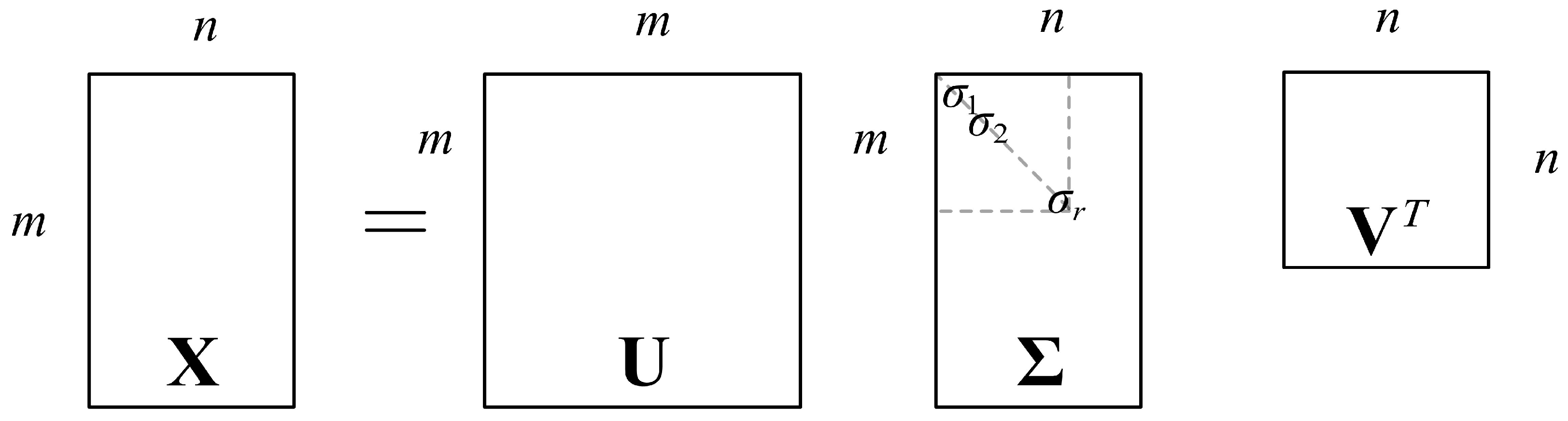
• SVD: perform SVD decomposition on the matrix ${\mathbf{X}}^{\prime }$ to obtain the matrix $\mathbf{U}$ and the singular value matrix $\Sigma$.
• Metric calculation: compute the normalized energy $p_i={\sigma }_i^2/\sum {\sigma }_j^2$ and total information entropy $H=-\sum p_{i}log\left(p_i\right)$.
• Iterative k-value search: determine the minimal k satisfying ${\sum }_{i=1}^k-p_{i}log\left(p_i\right)/H>0.9$ by cumulative entropy proportion analysis. Construct a $k\times k$ diagonal matrix ${\Sigma }_k$.
• Signal reconstruction: select the first k columns in the matrix $\mathbf{U}$ to construct a $m\times k$ matrix ${\mathbf{U}}_k$, the first k rows in the matrix $\mathbf{V}$ to construct a $k\times n$ matrix ${\mathbf{V}}_k$, and obtain the final denoised signal matrix ${\mathbf{X}}_k={\mathbf{U}}_k{\Sigma }_k{{\mathbf{V}}_k}^{\mathrm{T}}$.

The entropy-based singular value selection method establishes a theoretical foundation for singular value determination from an information-theoretic perspective. Compared to fixed threshold approaches, this method dynamically senses signal complexity and achieves SNR-adaptive correlation. Under high SNR conditions, the signal energy is highly concentrated and the information entropy is low, so only a few singular values need to be retained to capture the main features. In low SNR scenarios, the signal energy distribution is more dispersed and the entropy value increases, so more singular values are automatically selected for retention to enhance the signal structure recovery capability. Different k values are calculated under different SNR conditions, which reflects the dynamics and is more in line with the non-ideal conditions in real wireless communications.

4. Proposed Framework

Based on the SVD signal denoising process, a three-channel convolutional gated recurrent unit deep neural network (TCGDNN) is constructed. The framework fully integrates entropy-based SVD denoising, three-channel spatial feature extraction, temporal feature extraction, and fully connected classification modules. By extracting key signal features through three-channel input, the model’s discriminative ability and generalization performance are enhanced, achieving more accurate modulation classification. The structure of the proposed framework is illustrated in Figure 3.

4.1. Three-Channel Spatial Feature Extraction Module

The three-channel spatial feature extraction module consists of four 1D convolutional layers (Conv1, Conv2, Conv3, and Conv4), four 2D convolutional layers (Conv5, Conv6, Conv7, and Conv8), and an improved SE block. First, the signal matrix ${\mathbf{X}}_k$ obtained after SVD denoising is divided into three channels: Input I, Input Q, and Input A/P. I is input to Conv1 and Conv2, Q is input to Conv3 and Conv4, and A/P is input to Conv7. Conv1 and Conv3 both have 50 convolution kernels of size 1 × 5; Conv2 and Conv4 both have 50 convolution kernels of size 1 × 3. In particular, the four 1D convolutional layers all use “casual” padding to make sure the framework cannot violate the ordering in which we model the separated channel data. Later, Conv1 and Conv3 are fused into Concatenate1, Conv2 and Conv4 are fused into Concatenate2 and input into Conv5 and Conv6 to mine spatial correlation. The 1D convolutional layers process the temporal relationship between I and Q signals, extracting spatial features while deepening the feature fusion between signals [22]. The 2D convolutional layers extract the spatial features of amplitude and phase signals. Through serial splicing and parallel interaction, this multi-channel input and processing structure captures input representation features of different scales and makes full use of the complementary information of I, Q, and A/P multi-channel data.To strengthen the focus on feature information and improve network performance, a channel attention mechanism is added, namely the improved SE block.

The traditional SE block improves the feature expression capability of neural networks by modeling the relationship between channels, thereby improving the model performance [23], as shown in Figure 4. For the input feature map $\mathbf{U}=\left[{\mathbf{u}}_1,{\mathbf{u}}_2,\dots ,{\mathbf{u}}_c\right]$, H and W represent the height and width of a channel and C represents the number of channels. Its core consists of three modules: the Squeeze module ${\mathbf{F}}_{sq}\left(·\right)$, the Excitation module ${\mathbf{F}}_{ex}\left(·,\mathbf{W}\right)$, and the Scale module ${\mathbf{F}}_{scale}\left(·,·\right)$.

The Squeeze module compresses the $W\times H\times C$ feature map $\mathbf{U}$ containing global information into a $1\times 1\times C$ feature vector $\mathbf{z}$ through using global average pooling (GAP). This compresses the two-dimensional spatial features into a one-dimensional global description. By taking the average height and width dimensions of the feature map, the feature map is converted into a vector containing only channel information, increasing the expressive ability of the convolutional neural network. The c-th element of $\mathbf{z}$ is calculated by:

$$z_c={\mathbf{F}}_{sq}\left({\mathbf{u}}_c\right)={\displaystyle \frac{1}{H\times W}}\sum _{i=1}^H\sum _{j=1}^W{u}_c(i,j).$$

(11)

The Excitation module mainly includes FC layers and activation function layers. A gate mechanism consisting of two FC layers is adopted. The first FC layer compresses C channels into $C/r$ channels to achieve feature dimensionality reduction and then enhances the nonlinear expression capability through an ReLU activation function. The second FC layer restores the number of channels to C, and a Sigmoid activation function generates a $1\times 1\times C$ dynamic weight vector $\mathbf{s}$, which characterizes the weights of the C feature maps in $\mathbf{U}$, where r is the compression ratio.

$$\mathbf{s}={\mathbf{F}}_{ex}(\mathbf{z},\mathbf{W})=\sigma \left({\mathbf{W}}_2\delta \left({\mathbf{W}}_1\mathbf{z}\right)\right),$$

(12)

where ${\mathbf{W}}_1$ and ${\mathbf{W}}_2$ are the weight matrices of the FC layer, $\delta \left(·\right)$ is the ReLU activation function, and $\sigma \left(·\right)$ is the Sigmoid activation function.

In the Scale module, the previously obtained attention weights are applied to the features of each channel. The weights $s_c$ are multiplied one by one with each channel of the original feature map $\mathbf{U}$, achieving the redistribution of channel features and obtaining the final output $\tilde{\mathbf{X}}=\left[{\tilde{\mathbf{x}}}_{\mathbf{1}},{\tilde{\mathbf{x}}}_{\mathbf{2}},\dots ,{\tilde{\mathbf{x}}}_{\mathbf{c}}\right]$. The specific expression is:

$${\tilde{\mathbf{x}}}_c={\mathbf{F}}_{scale}({\mathbf{u}}_c,s_c)=s_c{\mathbf{u}}_c.$$

(13)

For the above traditional SE block, it extracts the global features of each channel through GAP and then learns the channel weights through the FC layers, thereby enhancing the model’s ability to focus on different channels. In order to further improve the performance of the SE block and reduce computational complexity, an improved version of the SE block is proposed. The main work is as follows:

• Propose a bimodal feature extraction strategy that combines global maximum pooling (GMP) and GAP to more comprehensively extract channel features.
• Introduce a batch normalization (BN) layer in the Excitation module to effectively alleviate parameter coupling issues in the FC layers, further improving training stability and efficiency.
• Reconstruct the network topology of the Excitation module to build a composite excitation structure containing multi-level nonlinear transformations, enabling refined modeling of high-order correlations between channels.

The channel attention mechanism dynamically adjusts the importance of channel features through three steps: Squeeze, Excitation, and Scale, as shown in Figure 5a. The improved SE block introduces GMP in the Squeeze module. GAP is mainly used to capture the average features of each channel, while GMP can extract the significant parts of the features in the channel. By fusing the results of GAP and GMP, a more comprehensive channel feature representation can be obtained. This fusion strategy not only enables the model to simultaneously utilize the average information and the most significant information of the channel but also improves the model’s flexibility and accuracy in capturing complex dependencies between channels. The traditional SE block only uses GAP, which may cause information loss when processing some complex input signals. The improved SE block effectively avoids this problem by fusing both pooling methods. After the FC layer of the Excitation module, the BN layer is introduced. The BN layer can mitigate potential gradient vanishing or exploding issues during training and accelerate the convergence process. By standardizing the output of each layer, the BN layer helps stabilize training and improve the training efficiency of the network. In addition, the BN layer can also reduce the risk of overfitting to a certain extent. Meanwhile, the improved block reconstructs the nonlinear link design of the excitation module. The Excitation module of the traditional SE block only generates channel weights through two FC layers, with limited linear expressive capability. The improved version extends the Excitation module into a multi-level composite structure, as shown in Figure 5b. By introducing additional nonlinear activation and normalization operations, the modeling ability of high-order dependencies between channels is enhanced.

4.2. Temporal Feature Extraction Module

This module has two GRU layers with 128 units each, which can effectively process sequential data to extract temporal correlations. GRU is a simplified recurrent neural network (RNN). Compared with long short-term memory networks (LSTMs), its structure is more concise, yet it can achieve similar performance in many tasks [24]. GRU controls information flow through the Update Gate ($z_t$) and Reset Gate ($r_t$), allowing the network to effectively learn long-term dependencies in time series.

The core of the GRU layer lies in its gating mechanism, which includes $r_t$ and $z_t$, as shown in Figure 6. These gates are used to adjust how to update the hidden state. It has only two gates; $r_t$ controls the influence between the current input and the past state, while $z_t$ determines how much old memory will be retained and how much new memory will be added. The execution steps are shown as follows:

1. Update Gate:

The update gate determines the update degree of the hidden state at the current moment. Its function is to control the proportion of past memories in the current hidden state. The closer the value $z_t$ is to 1, the more past information is retained; when $z_t$ approaches 0, it means that the current state will be determined by the new input $x_t$. The calculation formula is:

$$z_t=\sigma \left(W_z·[h_{t-1},x_t]\right),$$

(14)

where $x_t$ is the input of the current time step, $h_{t-1}$ is the hidden state of the previous time step, and $W_z$ is the weights of the update gate.

2. Reset Gate:

The reset gate controls how to integrate the previous state $h_{t-1}$ into the calculation of the current time step. Its function is to control how much information in the hidden state $h_{t-1}$ will be overwritten by the current input $x_t$. When $r_t$ is 0, it means that the past information is completely forgotten; when $r_t$ is 1, it means that the past memory is completely retained. The calculation formula is:

$$r_t=\sigma \left(W_r·\left[h_{t-1},x_t\right]\right),$$

(15)

where $x_t$ is the input of the current time step, $h_{t-1}$ is the hidden state of the previous time step, $W_r$ is the weights of the reset gate, and $\sigma$ is the sigmoid activation function, which outputs a value in the range [0, 1].

3. Candidate Hidden State:

Candidate hidden state represents the “candidate memory” of the current time step, but it will not directly become the final hidden state. It determines the final hidden state together with the hidden state of the previous moment. ${\tilde{h}}_t$ is the calculation of the candidate memory state at the current moment, which is jointly determined by the current input $x_t$ and the previous hidden state $h_{t-1}$:

$${\tilde{h}}_t=tanh\left(W_h·\left[r_t\odot h_{t-1},x_t\right]\right),$$

(16)

where $r_t$ is the reset gate calculated previously, ⊙ is the Hadamard product, which means element-wise multiplication, $W_h$ is the weights of the candidate hidden state, and tanh is the hyperbolic tangent function, which limits the value to the range [−1, 1].

4. Hidden state update:

The final hidden state $h_t$ is the output of the current time step. It decides whether or not to use the current candidate hidden state ${\tilde{h}}_t$ by updating the gate $z_t$:

$$h_t=\left(1-z_t\right)\odot h_{t-1}+z_t\odot {\tilde{h}}_t.$$

(17)

The formula shows that when $z_t$ approaches 1, the current hidden state $h_t$ depends more on the previous state $h_{t-1}$; when $z_t$ approaches 0, the current hidden state $h_t$ will completely depend on the candidate hidden state ${\tilde{h}}_t$, that is, the current input $x_t$ will have a greater update on the hidden state.

Figure 6. GRU unit structure.

Figure 6. GRU unit structure.

GRU is a more efficient recurrent neural network structure than the traditional LSTM and is particularly suitable for processing temporal data with long-term dependencies. Through this structure, the dynamic changes of the signal can be captured in the time domain. In the first half of the model, the improved SE block extracts the spatial features of each channel through channel weighting, while the GRU layers focus on extracting the dynamic features of the signal from the time domain. By combining the two, the model can extract information in both time and feature dimensions, thereby improving the representation ability of signals with temporal correlation and enhancing classification performance.

4.3. Fully Connected Classification and Recognition Module

For mapping features to a more separable space, two FC layers are added to the model, one with 256 neurons and the other with 128 neurons. This helps extract high-level features of the input data. Scaled exponential linear (SeLU) activation is used to avoid gradient disappearance and stabilize the training process. To prevent overfitting, 20% dropout layers are added after the FC layers. The layers randomly discard neurons, thereby enhancing the model’s generalization ability. The output layer uses Softmax and has 11 neurons to ensure that the output is a probability distribution, representing 11 modulation methods. The maximum probability value corresponds to the prediction result.

5. Simulation Experiment and Performance Analysis

5.1. Dataset

The dataset used in this paper is the RML2016.10a modulation dataset released by O’Shea in 2016 [4], which contains eight digital modulation schemes (8PSK, BPSK, CPFSK, GFSK, PAM4, 16QAM, 64QAM, QPSK) and three analog modulation schemes (AM-DSB, AM-SSB, WBFM). These signal samples are generated in a harsh simulated propagation environment, affected by factors such as additive white noise, multi-path fading, sampling rate offset, and center frequency offset. The SNR ranges from −20 to 18 dB, with 2 dB step size and a total of 220,000 samples. This dataset encompasses a variety of wireless communication modulation schemes and diverse channel conditions, simulating the real electromagnetic environment in

Table 1. Dataset Parameters.

Related Parameters	Parameter Settings
Data format	IQ data format; 2 × 128
Number of samples	220,000
Sampling frequency	1 MHz
Modulation schemes	11 classes: 8PSK, BPSK, CPFSK, GFSK, PAM4, 16QAM, 64QAM, QPSK, AM-DSB, AM-SSB, WBFM
SNR (dB)	$-20:2:18$
Channel environment	Additive Gaussian white noise, selective fading (Rice + Rayleigh)

. In order to improve the efficiency and performance of model training, all signal samples are normalized to ensure that the samples are compared at the same scale.

5.2. Experimental Environment

In the dataset, each modulation scheme is randomly divided into training, testing, and validation sets in an 8:1:1 ratio. The Adam optimizer with an initial learning rate of 0.001 is used in the training phase, and cross entropy is employed as the loss function. To optimize the training process, if the validation loss does not improve in 10 consecutive epochs, the learning rate is reduced to 0.5 times its original value; if no improvement is observed for 50 epochs, the training is terminated early to avoid overfitting. All experiments are conducted in TensorFlow using the Keras library, supported by NVIDIA CUDA, with a GeForce RTX 2050 GPU and an AMD Ryzen 7 6800H CPU.

5.3. Comparative Experiment

The experiment selected CNN [25], GRU2 [26], DAE [27], LSTM2 [28], ResNet, and CLDNN in [29] as comparative simulation models. The simulation results of different models on the dataset are shown in

Table 2. Simulation results of different models.

Network Model	Parameters	Training Epochs	Single Signal Test Time/ms	0–18 dB
				Average Classifica- tion Accuracy	Average Probability of 16QAM Being Confused with 64QAM	Average Probability of 64QAM Being Confused with 16QAM	Average Confusion Probability
TCGDNN	489,341	95	40.808	91.16%	3.80%	10.40%	7.10%
CLDNN	517,643	188	38.280	82.23%	55.60%	14.00%	34.80%
CNN	1,592,383	154	29.988	82.66%	56.90%	36.10%	46.50%
ResNet	3,098,283	125	44.333	82.55%	71.30%	16.60%	43.95%
GRU2	151,179	106	33.267	84.05%	48.10%	38.10%	43.10%
DAE	1,063,659	242	46.358	85.75%	35.50%	38.10%	36.80%
LSTM2	201,099	114	30.400	83.82%	62.90%	28.20%	45.55%

.

Compared with other existing models, the model proposed in this paper shows significant advantages in modulation recognition tasks. TCGDNN has 489,341 parameters, which is much less than CNN and DAE. In terms of accuracy, the average classification accuracy in the SNR range of 0 dB to 18 dB is 91.16%, showing strong performance, which is 5.41% to 8.93% higher than other models. In addition, by observing the number of training epochs and single signal inference time, it can be found that the TCGDNN has significantly fewer training epochs than other models, only 95 rounds, showing high training efficiency. Its single signal inference time is 40.808 ms, which is at a medium level compared with other models. Although the advantage of single signal inference time is not outstanding, its average classification accuracy and high-order signal discrimination are excellent, which can effectively make up for the disadvantages in time performance. Therefore, considering the training overhead, inference efficiency, and classification accuracy, TCGDNN still has strong practical value and promotion potential in practical applications.

Experimental results show that the signal recognition accuracy of CNN and CLDNN is significantly lower than that of the other networks. This is mainly due to the relatively simple network structures of these two networks. CNN only extracts the frequency domain features of the signal and lacks the acquisition of time-series-related features. The CLDNN network combines CNN, LSTM, and fully connected layers. It theoretically has a certain ability to extract spatiotemporal features. However, its convolutional layer design is shallow, and its feature extraction capability is limited, making it difficult to capture multi-scale feature changes in complex modulated signals. Both of them only use the original I/Q signal as input, lacking the modeling of key features such as amplitude and phase. Both GRU2 and LSTM2 convert the amplitude and phase of I/Q data and send them into the network model as input data. Although this improves the integrity of the input information to a certain extent, their network structure mainly relies on RNN units to extract the time-domain features of the signal and lacks an effective spatial feature extraction mechanism, resulting in limited modeling capabilities for short-term mutation features. In contrast, TCGDNN fuses multi-dimensional information such as I/Q and amplitude phase through multi-channel input and combines CNN with a two-layer GRU to enhance the extraction of key features and timing modeling. ResNet introduced residual connections based on CNN. However, reference [29] pointed out that the ResNet they designed only contained four convolutional layers and the network depth was shallow, which limited its ability to use the residual structure to improve the performance of the model, resulting in low recognition accuracy. The DAE structure proposed in [27] is similar to the basic autoencoder. Its training objective focuses on reconstructing the noisy signal and is more concerned with restoring the global signal structure. It often lacks the ability to extract subtle differences between modulation modes. Reference [20] points out that DAE is prone to fall into local optimality and suffers from performance degradation. When the SNR is high, the network is prone to overfitting the reconstruction characteristics and ignoring the discriminative information required to distinguish different modulation types. The model proposed in this paper achieves noise reduction through entropy-based SVD at the front end, avoiding the problem of reconstruction misleading in the end-to-end structure.

It is noteworthy that the proposed model exhibits obvious advantages in the distinction between 16QAM and 64QAM. According to the experimental results, within the 0–18 dB range, the average confusion probability between 16QAM and 64QAM in the proposed model is 7.10%, which is much lower than that of other models. Compared with the average confusion probability of other models, it is reduced by 27.70% to 39.40%.

These experimental results indicate that the proposed model is superior to other models in terms of accuracy, and also shows significant advantages in distinguishing high-order QAM signals. This further validates the robust performance of the proposed model in signal modulation recognition tasks, especially when processing high-order signals such as 16QAM and 64QAM, which can effectively reduce confusion and enhance signal recognition accuracy.

The recognition rate curves of CNN, GRU2, CLDNN, ResNet, DAE, LSTM2, and the proposed model TCGDNN for 11 types of signals at different SNR are shown in Figure 7.

As can be seen from Figure 7, when the SNR is lower than −4 dB, the recognition accuracy of the comparison model and the proposed model is not good; as the SNR increases, the noise and random error of the input data decreases, the quality of the signal is higher, and the network is easier to learn and recognize accurately, thereby improving the recognition rate. When the SNR is higher than −4 dB, the recognition accuracy of the TCGDNN model proposed in this paper is significantly better than that of other comparison models, and the recognition curve is stable at around 92%.

The recognition effect of CLDNN is weaker than that of other models, with the highest recognition rate of 85.36%, 83.81% for CNN, and 83.68% for ResNet. The three only perform two-dimensional convolution processing on I/Q data, and the network models are relatively shallow. The information obtained by the convolution layer is mainly limited to local spatial features, which makes it difficult to fully capture the temporal changes and complex feature distribution of the signal, resulting in weak feature extraction capabilities. Both GRU2 and LSTM2 models have strong time-series modeling capabilities but are still inferior to TCGDNN in terms of feature fusion and noise resistance. The highest recognition rates are 85.18% and 85.27%, respectively. Since the two structures are similar, the recognition results are also slightly different. DAE trains an autoencoder based on LSTM to reconstruct the original received signal, but it lacks the ability to extract subtle differences between modulation modes, so the maximum recognition rate is only increased to 87.72%. However, TCGDNN makes up for the shortcomings of other models. First, entropy-based SVD is introduced to the signal at the input end, and then three-channel convolutional layers are used to learn I, Q, and amplitude phase features, and the GRU module is introduced to realize time–frequency joint modeling. On this basis, the additional improved attention mechanism can learn the subtle differences between different signals, thus achieving a maximum recognition accuracy of 92.54%, which is the best performance among all compared models.

To provide a more detailed analysis of the model’s recognition performance for different modulation signals, the confusion matrices of CNN, ResNet, DenseNet, CLDNN, LSTM2, GRU2, and TCGDNN at an SNR of 4 dB are presented. The clarity of the diagonal in the confusion matrix is an important metric for evaluating the recognition effect of the algorithm. It reflects the algorithm’s ability to recognize each modulation signal in the dataset. A more obvious diagonal with darker grid colors indicates stronger recognition capability for each signal. The confusion matrices of each model when the SNR is 4dB are shown in Figure 8.

From the figures, it can be observed that, at an SNR of 4 dB, the confusion matrix of the proposed model has fewer clutter blocks and achieves a highest recognition accuracy. In contrast, the confusion matrices of other models have clutter blocks on the diagonal, indicating a gap in their recognition capabilities. The most notable issue is that traditional models perform poorly in distinguishing 16QAM and 64QAM. Since these two modulation schemes are based on amplitude and phase, some symbol characteristics are similar, which increases the difficulty of distinction. However, TCGDNN performs well in recognizing 16QAM and 64QAM, highlighting its ability to handle complex modulation schemes.

It can be seen that AM-DSB and WBFM are easily confused. The main reason for this is that the two are highly similar in spectral characteristics: both show symmetrical sideband structures and lack obvious carrier components. Especially when the frequency modulation index of WBFM is low, its spectral envelope is very close to AM-DSB. In addition, both types of signal in the dataset are derived from analog audio sampling and have silent segments, which further weakens their discriminative features. Due to the overlap in essential characteristics of the two, even under high SNR conditions, it is still difficult for the model to accurately distinguish them. This is also a common challenge faced by current deep-learning models in modulation recognition.

5.4. Ablation Experiment

In order to verify the impact of entropy-based SVD denoising and improved SE block on model performance, this section conducts ablation experiments. The experiments utilize TCGDNN-A (the improved SE block and SVD denoising is removed from TCGDNN), TCGDNN-B (the improved SE block is removed), TCGDNN-C (the improved SE block replaced by the CBAM attention block [30]), TCGDNN-D (the traditional SE block is used), and the complete model TCGDNN.

Table 3. Results of ablation experiments.

	0–18 dB
Network Model	Average Classification Accuracy	Average Probability of 16QAM Being Confused with 64QAM	Average Probability of 64QAM Being Confused with 16QAM	Average Confusion Probability
TCGDNN	91.25%	3.80%	10.40%	7.10%
TCGDNN-A	89.35%	13.90%	24.10%	19.00%
TCGDNN-B	89.95%	7.30%	27.60%	17.45%
TCGDNN-C	85.96%	11.90%	43.20%	27.55%
TCGDNN-D	89.88%	7.00%	24.90%	15.95%

shows the ablation experiment results of these five network models on the dataset.

The experimental results show that the average recognition rate and high-order signal discrimination of TCGDNN-B are better than those of TCGDNN-A. This indicates that SVD plays a critical role in noise reduction and feature extraction in the signal preprocessing stage and improves the model’s ability to distinguish complex modulation types.

Comparative analysis of TCGDNN-B, TCGDNN-C, and TCGDNN-D reveals the improved SE module’s contribution to higher-order signal differentiation. Although the CBAM attention module (TCGDNN-C) integrates GMP and spatial attention mechanisms, it exhibits the lowest average recognition accuracy in ablation experiments. This may stem from CBAM’s insensitivity to weakly represented time–frequency features in high-noise, small-sample scenarios, limiting critical feature enhancement. Additionally, CBAM’s structural complexity increases model parameters and computational overhead, diminishing practical deployment advantages. Consequently, this study is more suitable to introduce SE attention mechanism to make subtle distinctions.

The dual-pooling-enhanced SE module, leveraging multi-scale feature fusion and dynamic channel weighting, precisely focuses on symbol spacing and phase transitions in high-order signals. It achieves a 7.10% confusion probability between 64QAM and 16QAM, outperforming TCGDNN-C (27.55%) and TCGDNN-D (15.95%). These results confirm that the improved SE block effectively reduces confusion in high-order QAM signal classification.

In summary, the synergy of entropy-based SVD denoising and improved SE block significantly improves the model’s classification performance for complex modulated signals: SVD provides pure feature input for the model through front-end denoising, while the improved SE block further enhances the ability to distinguish high-order signals through back-end feature focusing. The combination of the two enables the complete model to maintain a high recognition accuracy and a low confusion probability in a high-noise environment, verifying its effectiveness in the task of high-order QAM signal classification.

Figure 9 shows the recognition accuracy curves of the five models on the dataset. When the SNR exceeds 8 dB, the recognition accuracy of the TCGDNN stabilizes around 92%.

6. Discussion

6.1. Technical Features and Contributions

The TCGDNN model is proposed in this study. Based on entropy-based SVD preprocessing, it integrates a three-channel convolutional GRU with an improved SE attention mechanism for automatic modulation recognition. This design enables accurate identification of modulation signals. Its core technical features are summarized as follows.

First, an entropy-based SVD method is employed for denoising the received signals. Unlike conventional SVD denoising approaches that rely on fixed singular value thresholds [31,32], this work introduces an adaptive singular value selection mechanism based on information entropy. The value of k is computed dynamically from entropy, enabling SNR adaptivity. This approach effectively suppresses channel noise and enhances principal signal components, providing a more robust input for subsequent feature extraction. Compared with the direct modeling of raw signals [33,34,35], it improves model discriminability.

Second, a three-channel input structure is designed to incorporate I, Q, and A/P information from the received signals. One-dimensional convolutional layers extract local temporal features from I and Q while preserving inter-channel complementarity. Two-dimensional convolutional layers are applied to the A/P channel to capture spatial correlations. Through serial and parallel fusion strategies, this module further expands feature dimensions. In serial fusion, multiple convolution outputs are concatenated to enhance multidimensional feature representation. In parallel fusion, convolution results from different branches interact, improving feature utilization across channels. Compared with prior models relying on single-channel inputs [36], this design offers structural and representational improvements, demonstrating enhanced robustness and recognition performance.

Third, an improved SE attention mechanism is integrated into the spatial feature extraction module to enhance key feature representation. Compared with the conventional SE module [37], GMP is added to jointly capture overall trends and abrupt features during channel weighting. This dual-pooling fusion enhances sensitivity to subtle variations in high-order modulation signals, improving their recognition and overall feature expressiveness. Furthermore, a GRU module is employed to model temporal dependencies, strengthening the extraction of modulation dynamics.

Compared with existing models, TCGDNN offers significant contribution across multiple dimensions. First, in terms of average recognition accuracy, it outperforms six conventional deep models by a margin of 5.41% to 8.93%. Second, and more importantly, it improves the distinguishability of high-order signals, reducing average confusion probability by 27.70% to 39.40%. These improvements mainly result from entropy-based SVD preprocessing, which enhances signal quality; the three-channel convolution structure, which effectively fuses time and frequency domain features; and the improved SE block, which strengthens key feature perception.

The proposed model achieves substantial progress in structural design and feature modeling, demonstrating strong robustness and recognition capability—especially in distinguishing high-order modulation types such as 16QAM and 64QAM.

6.2. Limitations and Prospects

Although achieving promising recognition performance, this study has inherent limitations. The proposed three-channel feature extraction architecture integrates 1D and 2D convolutional operations to effectively capture temporal, spectral, and time–frequency joint features, demonstrating robust performance under typical channel conditions. However, its lack of explicit modeling for inter-channel nonlinear dependencies may constrain feature interaction capability in complex high-order scenarios, particularly presenting recognition challenges in low SNR environments.

The model achieves strong differentiation for most signals, particularly excelling in high-order modulation recognition, but the persistent confusion between AM-DSB and WBFM signals remains notable. This phenomenon stems from their spectral morphology similarity, resulting in elevated confusion rates. Such AM-DSB and WBFM ambiguity constitutes an intrinsic challenge in current modulation classification research.

We employ the widely adopted RML2016.10a dataset, encompassing diverse modulation types and typical channel models (AWGN, Rayleigh fading) for comprehensive evaluation. However, it excludes practical non-ideal impairments like adjacent-channel interference, frequency offsets, and parasitic coupling, partially constraining adaptability assessment in complex real-world scenarios.

Future research could focus on the following aspects. First, introduce cross-channel feature interaction mechanisms, such as an attention-guided feature crossing network, to enhance the nonlinear interaction expression between features. Second, adopt more complex public datasets (such as RML2018.01a) or simulate the actual imperfections of the receiving track systems. Build a simulated communication environment with real interference, so as to comprehensively evaluate and improve the generalization ability of the model under complex conditions. Third, for hard-to-classify modulation types, we will focus on improving the discrimination of WBFM and AM-DSB signals through the combination of further signal preprocessing and feature extraction techniques, as well as possible deep-learning methods, thereby improving the accuracy and performance of signal classification.

7. Conclusions

In this paper, we propose an innovative modulation recognition algorithm based on deep learning, which combines entropy-based SVD denoising technology and an improved SE attention mechanism. It processes I and Q signals using 1D convolutional and A/P signals using 2D convolutional to extract more effective features. The model achieves a good balance between accuracy and efficiency. Under different SNR conditions, the proposed algorithm shows stronger robustness and adaptability than traditional methods, especially in the recognition accuracy of 16QAM and 64QAM modulated signals.

Our study achieves a good balance between accuracy and efficiency by introducing a lightweight, robust automatic modulation recognition model. The proposed algorithm demonstrates stronger adaptability and robustness under varying SNR conditions compared to traditional methods, particularly in distinguishing 16QAM and 64QAM. This research responds to the growing demand for models that combine high recognition performance with lightweight architecture in modulation classification. Furthermore, it provides theoretical support and methodological guidance for future wireless signal recognition tasks under complex communication environments, showing promising potential for practical engineering applications and further academic exploration.

References

1. Liu, X.; Li, C.J.; Jin, C.T.; Leong, P.H.W. Wireless Signal Representation Techniques for Automatic Modulation Classification. IEEE Access 2022, 10, 84166–84187. [Google Scholar] [CrossRef]
2. Jassim, S.A.; Khider, I. Comparison of Automatic Modulation Classification Techniques. J. Commun. 2022, 17, 574–580. [Google Scholar] [CrossRef]
3. Ding, R.; Zhang, H.; Zhou, F.; Wu, Q.; Han, Z. Data-and-knowledge dual-driven automatic modulation recognition for wireless communication networks. In Proceedings of the ICC 2022-IEEE International Conference on Communications, Seoul, Republic of Korea, 16–20 May 2022; IEEE: Piscataway, NJ, USA, 2022; pp. 1962–1967. [Google Scholar]
4. O’Shea, T.; West, N. Radio Machine Learning Dataset Generation with GNU Radio. In Proceedings of the GNU Radio Conference, Boulder, CO, USA, 12–16 September 2016; Volume 1. [Google Scholar]
5. O’Shea, T.J.; Roy, T.; Clancy, T.C. Over-the-air deep learning based radio signal classification. IEEE J. Sel. Top. Signal Process. 2018, 12, 168–179. [Google Scholar] [CrossRef]
6. Simonyan, K.; Zisserman, A. Very deep convolutional networks for large-scale image recognition. arXiv 2014, arXiv:1409.1556. [Google Scholar]
7. He, K.; Zhang, X.; Ren, S.; Sun, J. Deep residual learning for image recognition. In Proceedings of the IEEE Conference on Computer Vision and Pattern Recognition, Las Vegas, NV, USA, 27–30 June 2016; pp. 770–778. [Google Scholar]
8. Zeng, Y.; Zhang, M.; Han, F.; Gong, Y.; Zhang, J. Spectrum analysis and convolutional neural network for automatic modulation recognition. IEEE Wirel. Commun. Lett. 2019, 8, 929–932. [Google Scholar] [CrossRef]
9. Qi, P.; Zhou, X.; Zheng, S.; Li, Z. Automatic modulation classification based on deep residual networks with multimodal information. IEEE Trans. Cogn. Commun. Netw. 2020, 7, 21–33. [Google Scholar] [CrossRef]
10. Zhang, Z.; Luo, H.; Wang, C.; Gan, C.; Xiang, Y. Automatic modulation classification using CNN-LSTM based dual-stream structure. IEEE Trans. Veh. Technol. 2020, 69, 13521–13531. [Google Scholar] [CrossRef]
11. Kohler, M.; Ahlemann, P.; Bantle, A.; Rapp, M.; Weiß, M.; O’Hagan, D. Transfer learning based intra-modulation of pulse classification using the continuous Paul-wavelet transform. In Proceedings of the 2022 23rd International Radar Symposium (IRS), Gdansk, Poland, 12–14 September 2022; IEEE: Piscataway, NJ, USA, 2022; pp. 496–500. [Google Scholar]
12. Zheng, Y.; Ma, Y.; Tian, C. Tmrn-glu: A transformer-based automatic classification recognition network improved by gate linear unit. Electronics 2022, 11, 1554. [Google Scholar] [CrossRef]
13. Deng, W.; Wang, X.; Huang, Z.; Xu, Q. Modulation classifier: A few-shot learning semi-supervised method based on multimodal information and domain adversarial network. IEEE Commun. Lett. 2022, 27, 576–580. [Google Scholar] [CrossRef]
14. Parmar, A.; Divya, K.; Chouhan, A.; Captain, K. Dual-stream CNN-BiLSTM model with attention layer for automatic modulation classification. In Proceedings of the 2023 15th International Conference on COMmunication Systems & NETworkS (COMSNETS), Bangalore, India, 3–8 January 2023; IEEE: Piscataway, NJ, USA, 2023; pp. 603–608. [Google Scholar]
15. Xu, T.; Ma, Y. Signal automatic modulation classification and recognition in view of deep learning. IEEE Access 2023, 11, 114623–114637. [Google Scholar] [CrossRef]
16. Zheng, Q.; Tian, X.; Yu, Z.; Wang, H.; Elhanashi, A.; Saponara, S. DL-PR: Generalized automatic modulation classification method based on deep learning with priori regularization. Eng. Appl. Artif. Intell. 2023, 122, 106082. [Google Scholar] [CrossRef]
17. Jang, J.; Pyo, J.; Yoon, Y.I.; Choi, J. Meta-transformer: A meta-learning framework for scalable automatic modulation classification. IEEE Access 2024, 12, 9267–9276. [Google Scholar] [CrossRef]
18. An, Z.; Xu, Y.; Tahir, A.; Wang, J.; Ma, B.; Pedersen, G.F.; Shen, M. Physics-Informed Scattering Transform Network for Modulation Recognition in 5G Industrial Cognitive Communications Considering Nonlinear Impairments in Active Phased Arrays. IEEE Trans. Ind. Inform. 2024, 21, 425–434. [Google Scholar] [CrossRef]
19. Beard, J.K. Singular value decomposition of a matrix representation of the Costas condition for Costas array selection. IEEE Trans. Aerosp. Electron. Syst. 2020, 57, 1139–1161. [Google Scholar] [CrossRef]
20. Zhang, F.; Luo, C.; Xu, J.; Luo, Y.; Zheng, F.C. Deep learning based automatic modulation recognition: Models, datasets, and challenges. Digit. Signal Process. 2022, 129, 103650. [Google Scholar] [CrossRef]
21. Ba, Y.; Ping, Y.; Tianyao, Z. Radar emitter signal identification based on weighted normalized singular-value decomposition. J. Radars 2019, 8, 44–53. [Google Scholar]
22. Zhang, T.; Weng, H.; Yi, K.; Chen, C. OneDConv: Generalized convolution for transform-invariant representation. arXiv 2022, arXiv:2201.05781. [Google Scholar]
23. Hu, J.; Shen, L.; Sun, G. Squeeze-and-excitation networks. In Proceedings of the IEEE Conference on Computer Vision and Pattern Recognition, Salt Lake City, UT, USA, 18–22 June 2018; pp. 7132–7141. [Google Scholar]
24. Ballakur, A.A.; Arya, A. Empirical evaluation of gated recurrent neural network architectures in aviation delay prediction. In Proceedings of the 2020 5th International Conference on Computing, Communication and Security (ICCCS), Patna, India, 14–16 October 2020; IEEE: Piscataway, NJ, USA, 2020; pp. 1–7. [Google Scholar]
25. Tekbıyık, K.; Ekti, A.R.; Görçin, A.; Kurt, G.K.; Keçeci, C. Robust and fast automatic modulation classification with CNN under multipath fading channels. In Proceedings of the 2020 IEEE 91st Vehicular Technology Conference (VTC2020-Spring), Antwerp, Belgium, 25–28 May 2020; IEEE: Piscataway, NJ, USA, 2020; pp. 1–6. [Google Scholar]
26. Hong, D.; Zhang, Z.; Xu, X. Automatic modulation classification using recurrent neural networks. In Proceedings of the 2017 3rd IEEE International Conference on Computer and Communications (ICCC), Chengdu, China, 13–16 December 2017; IEEE: Piscataway, NJ, USA, 2017; pp. 695–700. [Google Scholar]
27. Ke, Z.; Vikalo, H. Real-time radio technology and modulation classification via an LSTM auto-encoder. IEEE Trans. Wirel. Commun. 2021, 21, 370–382. [Google Scholar] [CrossRef]
28. Rajendran, S.; Meert, W.; Giustiniano, D.; Lenders, V.; Pollin, S. Distributed deep learning models for wireless signal classification with low-cost spectrum sensors. arXiv 2017, arXiv:1707.08908. [Google Scholar] [CrossRef]
29. Liu, X.; Yang, D.; El Gamal, A. Deep neural network architectures for modulation classification. In Proceedings of the 2017 51st Asilomar Conference on Signals, Systems, and Computers, Pacific Grove, CA, USA, 29 October–1 November 2017; IEEE: Piscataway, NJ, USA, 2017; pp. 915–919. [Google Scholar]
30. Jin, X.; Ma, J.; Ye, F. Radar signal recognition based on deep residual network with attention mechanism. In Proceedings of the 2021 IEEE 4th International Conference on Electronic Information and Communication Technology (ICEICT), Xi’an, China, 18–20 August 2021; IEEE: Piscataway, NJ, USA, 2021; pp. 428–432. [Google Scholar]
31. Abdel-Galil, T.; El-Hag, A.H.; Gaouda, A.; Salama, M.; Bartnikas, R. De-noising of partial discharge signal using eigen-decomposition technique. IEEE Trans. Dielectr. Electr. Insul. 2008, 15, 1657–1662. [Google Scholar] [CrossRef]
32. Baglama, J.; Chávez-Casillas, J.A.; Perović, V. A hybrid algorithm for computing a partial singular value decomposition satisfying a given threshold. Numer. Algorithms 2024, 1–17. [Google Scholar] [CrossRef]
33. Hermawan, A.P.; Ginanjar, R.R.; Kim, D.S.; Lee, J.M. CNN-based automatic modulation classification for beyond 5G communications. IEEE Commun. Lett. 2020, 24, 1038–1041. [Google Scholar] [CrossRef]
34. West, N.E.; O’shea, T. Deep architectures for modulation recognition. In Proceedings of the 2017 IEEE International Symposium on Dynamic Spectrum Access Networks (DySPAN), Baltimore, MD, USA, 6–9 March 2017; pp. 1–6. [Google Scholar]
35. Perenda, E.; Rajendran, S.; Pollin, S. Automatic modulation classification using parallel fusion of convolutional neural networks. In Proceedings of the BalkanCom’19, Skopje, North Macedonia, 10–12 June 2019. [Google Scholar]
36. Zhang, F.; Luo, C.; Xu, J.; Luo, Y. An efficient deep learning model for automatic modulation recognition based on parameter estimation and transformation. IEEE Commun. Lett. 2021, 25, 3287–3290. [Google Scholar] [CrossRef]
37. Wu, X.; Wei, S.; Zhou, Y. Deep multi-scale representation learning with attention for automatic modulation classification. In Proceedings of the 2022 International Joint Conference on Neural Networks (IJCNN), Padua, Italy, 18–23 July 2022; IEEE: Piscataway, NJ, USA, 2022; pp. 1–8. [Google Scholar]
Figure 1. Singular value decomposition schematic.
Electronics 14 02233 g001
Figure 2. Entropy-based SVD denoising process.
Electronics 14 02233 g002
Figure 3. The structure of the proposed framework TCGDNN.
Electronics 14 02233 g003
Figure 4. Schematic diagram of the traditional SE block.
Electronics 14 02233 g004
Figure 5. Framework of original and improved SE Blocks: (a) traditional SE block. (b) the improved SE block.
Electronics 14 02233 g005
Figure 7. Recognition accuracy comparison between TCGDNN and other frameworks.
Electronics 14 02233 g007
Figure 8. Confusion matrices for different models: (a) CNN. (b) LSTM2. (c) CLDNN1. (d) DAE. (e) ResNet. (f) GRU2. (g) TCGDNN.
Electronics 14 02233 g008
Figure 9. Recognition accuracy comparison between five frameworks.
Electronics 14 02233 g009