Optimizing the Energy Efficiency of Electric Vehicles in Urban and Metropolitan Environments According to Various Driving Cycles and Behavioral Conditions

Abstract

Electric vehicles are transforming urban and metropolitan transportation, providing significant benefits to both the environment and society. However, the integration of electric vehicles necessitates a well-planned infrastructure, including a sufficient number of charging stations distributed at the local level, policies that encourage the purchase and operation of electric vehicles, and the active participation of local governments and the automotive industry. Investments in improved car technologies, as well as renewable energy sources, will be critical in the shift to more sustainable metropolitan regions that have reduced pollution. Computer simulation based on virtual models performs an important role in the optimization of urban and metropolitan traffic by allowing for the rapid prototyping of real vehicle models, as well as the implementation of a wide range of test scenarios in real time. Assisted driving functions are critical in adjusting optimal driving behaviors to each of the particular scenarios of urban and metropolitan traffic. The situations discussed in this study were derived from real-world traffic and implemented and simulated on virtual models in the CarMaker version 12 application. To calibrate electricity consumption in each of the metropolitan area’s sectors, driving cycles were embedded in the virtual model. These were allocated to component sectors based on the average travel speed and its variation.

1. Introduction

Electric vehicles are an innovative and environmentally friendly alternative for urban and metropolitan transportation, contributing to the reduction in pollution, noise, maintenance, and operating expenses while enhancing energy efficiency.

Electric vehicles are becoming increasingly prevalent in urban and metropolitan traffic because of their ecological, economic, and technological advantages, providing considerable benefits to congested urban areas while also posing issues that necessitate careful planning and management.

The advantages of incorporating electric vehicles into urban and metropolitan traffic are as follows [1,2,3]:

• Reduced atmospheric pollution because electric vehicles do not generate polluting contaminants: carbon monoxide (CO), nitrogen oxides (NO_x), particulate matter (PM), and greenhouse gases (GHGs);
• Noise pollution is reduced as a result of the quietness of electric motors and systems used in electric vehicles;
• Operating costs are reduced due to the excellent energy efficiency of the electric motors that equip electric vehicles and due to the low price of electricity (particularly energy from renewable sources) compared to the price of fossil fuels;
• Maintenance costs are lowered since the systems that equip electric vehicles are less complex;
• Access to restricted areas in historic urban centers, free parking, and public and/or private charging stations with preferential pricing for power;
• Reductions in taxes and assessments, as well as financial incentives to buy new electric vehicles.

The disadvantages of electric vehicles in urban and metropolitan traffic include the following [4,5]:

• Infrastructural development in the majority of major cities and a reduced number of public and private charging stations that may be insufficient to serve all electric vehicles;
• Increase in electricity consumption in national grids (at certain times of the day) as the number of electric vehicles grows;
• In comparison to vehicles equipped with conventional propulsion systems (internal combustion engines and hybrid propulsion systems), autonomy is limited;
• In comparison to vehicles powered by conventional or hydrogen fuel where refueling takes only a few minutes, fast charging in a short period of time for electric vehicles may be more expensive than an extended charge overnight;
• The initial cost was higher than conventional vehicles in similar categories;
• Environmental issues arising from the recycling of batteries, as well as the management of waste batteries.

The future of electric vehicles in urban and metropolitan traffic is dependent on the adoption and implementation of favorable government policies based on subsidies and fiscal incentives for the purchase of these vehicles, as well as restrictions and prohibitions imposed on polluting vehicles in metropolitan areas.

In addition, advanced and innovative technologies used in the automotive industry, such as battery production technologies, fuel cell systems, and so on, will have a significant impact on the transition from conventional to electric vehicles. This study’s relevance is highlighted by the rapid development of energy-oriented control systems in the electric vehicle domain, such as those discussed in [6,7], which focus on enhanced torque-vectoring for distributed drive architectures.

Adopting electric vehicles in urban and metropolitan traffic represents a critical step toward the development of sustainable metropolises, which require a mobility solution that, in addition to the benefits of environmentally friendly transportation with Zero Local Emissions (ZLEs), provides the possibility of traffic decongestion through the integration of mobility services such as car-sharing and/or ride-hailing.

The implementation of AI-based algorithms, such as the Tabu Search Algorithm, which employs Particle Swarm Optimization [8,9], has resulted in the efficient optimization of urban and metropolitan routes for electric vehicles, as demonstrated in real-world logistical scenarios.

Ran et al. [10] introduced an automated type of clustering algorithm, K-means, that incorporates the noise algorithm, Genetic Algorithm (GA), an Adaptive Fuzzy System (AFS), and the Ant Colony Optimization (ACO) algorithm, in addition to the algorithm for tracking global GPS (Global Positioning System) positions and optimizing urban vehicle traffic. The primary goal of the K-means algorithm is to identify economically feasible and spatially homogenous metropolitan areas for traffic routing. The optimal routes for vehicle movement are obtained by controlling traffic based on the GPS location information of a maximum number of vehicles in traffic, or by managing traffic in intersections [11].

Mirjalili et al. [12] proposed the metaheuristic Grey Wolf Optimizer (GWO) algorithm based on a dynamic mobility scenario inspired by nature, with floating options classified at the hierarchical level in making decisions about the fixed route, in order to provide quick and precise solutions to various traffic scenarios. The GWO is a hybrid optimization algorithm that uses machine learning (ML) methods based on the implementation of an Artificial Neuronal Network (ANN) [13], which uses information provided and shared by all participants in the traffic [14].

The Fast Firefly Algorithm (FFA) was introduced to address the difficult problem of solving Nondeterministic Polynomial (NP) time hardness using non-convex functions with equality and inequality constraints [15]. The algorithm employs a search based on a large number of solutions that provide base information, allowing for the algorithm’s mechanism to facilitate good learning for training the parameters required to make decisions in a distributed way to balance exploration and exploitation. Bazi et al. [16] proposed a fast FFA for reducing search space by randomly selecting a significant group of subjects in motion to cover the whole search space under consideration.

Artificial Bee Colony (ABC) [17] is an algorithm based on a solution to an optimization issue to identify resources where the number of subjects considered is equal to the number of solutions. Each topic under consideration is involved in the search process and ranks the best resources discovered. At the end of the search process, subjects share information on the position of memorated resources. In the field of mobility, the proposed algorithm provides routes that combine reduced travel time with the selection of optimal travel distances while managing participant interference through continuous communication [18].

In their work, the authors implemented the results of their studies based on some of the algorithms presented earlier in the virtual model developed in CarMaker using command and control tools such as IPGRoad, IPGDriver, traffic, environment, etc.

2. Materials and Methods

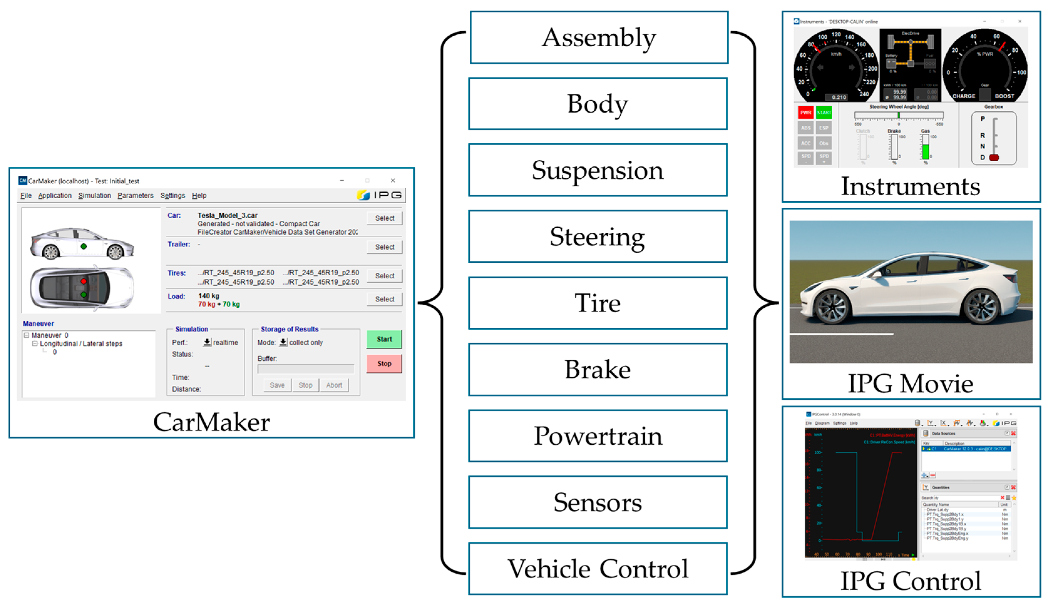
2.1. Simulation Platform

Computer simulation is used to simulate real-world studies in a virtual environment, using a theoretical model that represents a digital image of an existing physical model, and the process of computer simulation is used to develop and improve the quality of this model. The complexity of the virtual model must correspond to the reality of the evaluated model, as complicated as necessary but as simple as possible, so that the results obtained from computer simulations can be validated by experimental results [19].

CarMaker is a simulation platform used by a large number of automotive companies to create, test, and optimize virtual vehicle models in various architectural designs [20,21]. There are virtual vehicle models in the application library that contain predefined parameters of the real vehicle, such as dimensions, mass, aerodynamics, steering and suspension systems, engine characteristics, and driver assistance functions ADAS (Advanced Driver-Assistance System) (Figure 1).

According to [22], CarMaker is a versatile platform that allows for the development and real-time simulation of electric vehicles integrated into a virtual environment capable of simulating a variety of external factors such as meteorological conditions, various traffic scenarios, different driving behaviors for the virtual driver, the ability to define any type of vehicle, the digitization of any sector of Google Earth/Maps, etc. [23].

Realistic scenarios that may be defined in CarMaker allow for the assisted driving of virtual models using ADAS systems, which are connected via V2X (Vehicle-to-Everything) systems between vehicles and the intelligent environment.

Toth et al. [24] used measurements taken from real-world vehicle movements to create a simulation model that ensures compatibility with the real-world model for each driving scenario chosen.

Another advantage of CarMaker’s virtual models is that they allow for the real-time testing of sophisticated HiL (Hardware-in-the-Loop) systems [25], as well as the selection of simulated CAN (Controller Area Network) parameters.

The CarMaker platform has obtained ISO 26262 certification from TÜV Nord [26] for developing complex simulation solutions and validating virtual vehicle models, which is an important factor in the credibility of scientific research results based on simulation scenarios.

2.2. Selection of the Initial Data

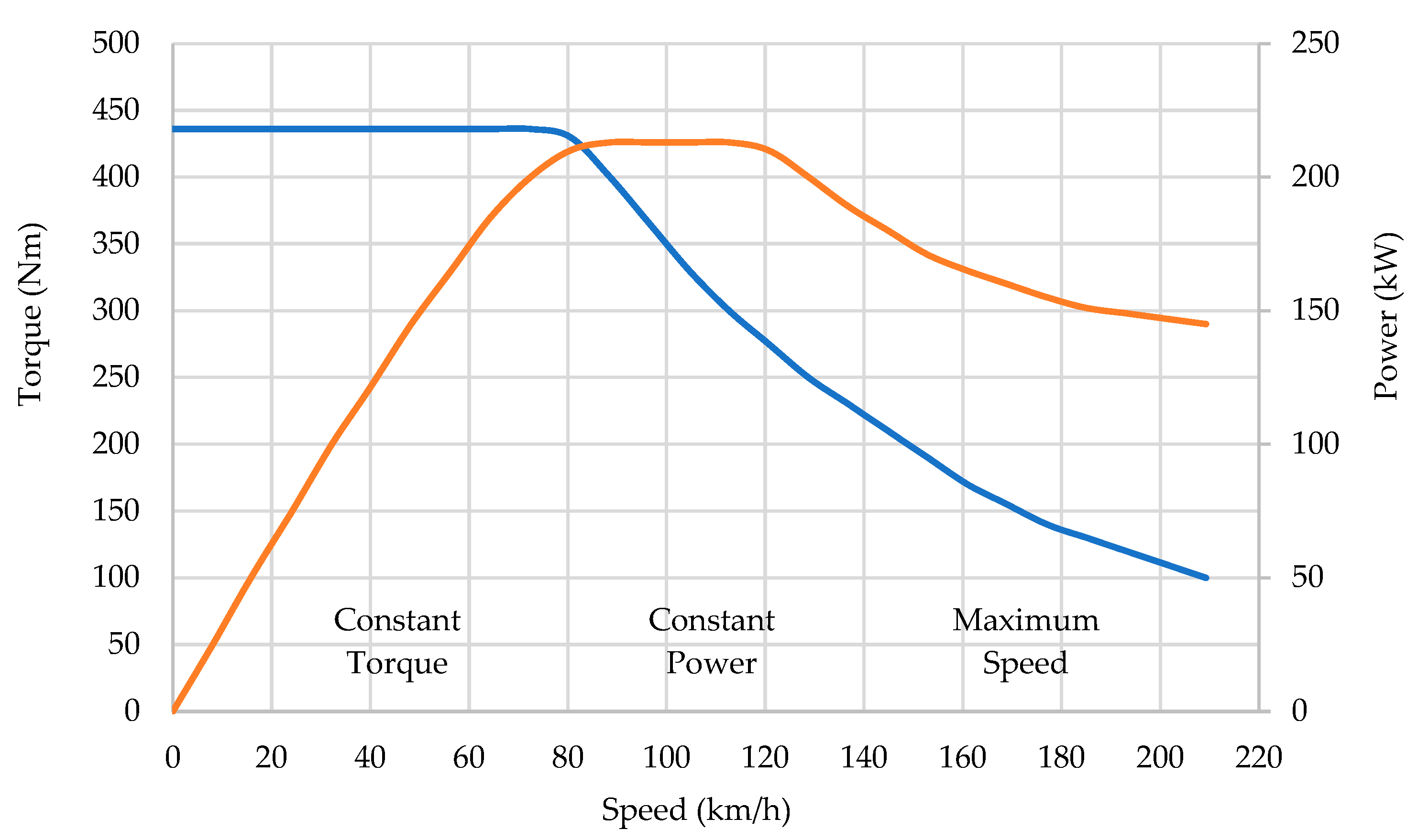
Electric Vehicle Characteristics and Performance

A Tesla Model 3 was used to perform tests and collect data on electric energy consumption and recovery in the metropolitan area under consideration. This vehicle model was used to create a virtual model, which is utilized in computer simulations.

The Tesla Model 3 is an electric vehicle that includes All-Wheel Drive (AWD) and two synchronous electric motors with permanent magnets. According to Tesla requirements [27],

Table 1. Tesla Model 3 operating performance was used to define the virtual vehicle model in CarMaker.

Parameters	Unit	Value
Maximum motor power (6000–9500 1/min)	kW	213
Maximum motor torque (0–5800 1/min)	Nm	436
Battery energy storage	kWh	78
Battery nominal voltage	VDC	357
Battery number of cells [28]	-	4416
Battery pack configuration (serial/parallel) [28]	-	96s46p
Rapid charging (supercharger V3 up to 282 km)	min	15
Energy consumption	kWh/km	0.14
Estimate range (EPA-FTP-75 range test [29])	km/kWh/km	488/0.16
Estimate range (WLTP range test [30])	km/kWh/km	528/0.15
Certified range (0 to 100 km/h)	s	5.2
Maximum speed	km/h	201

shows the main structural parameters of the powertrain group, and

Table 2. Tesla Model 3 dimensions and weights were used to define the virtual vehicle model in CarMaker.

Parameters	Unit	Value
Overall length	mm	4720
Overall width (including mirrors)	mm	2089
Overall height	mm	1442
Wheelbase	mm	2875
Overhang front/rear	mm	868/977
Ground clearance	mm	138
Track wheels front/rear	mm	1584/1584
Curb mass (no occupants and no cargo)	kg	1823
Technically permissible maximum laden mass	kg	2255
Maximum payload	kg	432

shows the vehicle’s dimensions and mass.

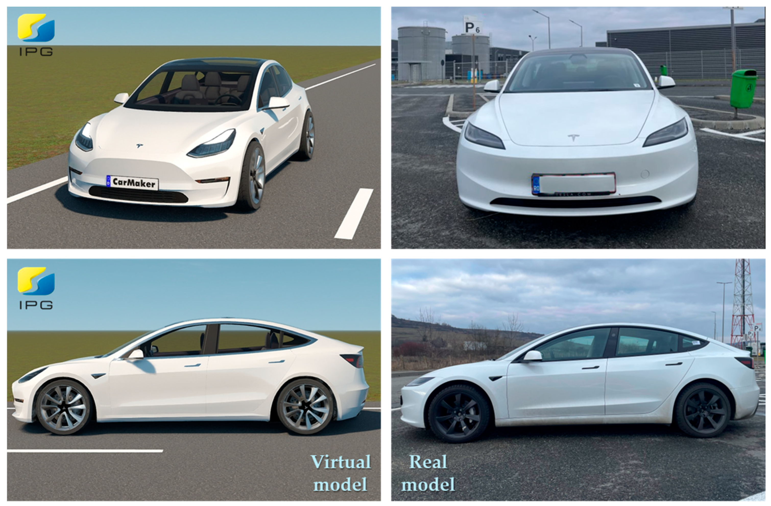
2.3. Virtual Model Development

2.3.1. Virtual Model for Electric Vehicle

The virtual model for the electric vehicle Tesla Model 3 was created in CarMaker (Figure 2) [31] using data extracted from the real model’s structural characteristics in addition to experimental determinations performed with the vehicle.

Computer simulations allow for high-precision results at a low cost, provided that the virtual model is validated through experimental determinations [32,33,34].

The torque/power characteristic (Figure 3) [35] indicates that the electric motors of the Tesla Model 3 operate at a constant torque, where the active power increases linearly as the torque increases, and at a constant power, where the torque changes in opposite relation to the torque of the motor. The power and moment characteristics of electric motors that will be determined in the development of a virtual vehicle model are constant torque, which indicates the maximum motor speed limited by the maximum current admissible, constant power, which indicates the maximum motor speed, and the maximum motor power, which decrease due to mechanical limitations [36].

The motor torque M_EM is calculated using the following equation [37,38]:

$$M_{EM}=M_{Max}\left(\omega \right)·{Load}_{EM}$$

(1)

where M_Max(ω) is the maximum motor torque for the electric motor/generator, and Load_EM is the electric motor’s load characteristic.

The power of an electric motor in the motor mode P_ElecMot and in the generator mode P_ElecGen is calculated using the following equations [37,38]:

$$P_{ElecMot}={\displaystyle \frac{M_{EM}·\omega }{{\eta }_{Mot}}}$$

(2)

$$P_{ElecGen}=M_{EM}·\omega ·{\eta }_{Gen}$$

(3)

where η_Mot represents motor efficiency and η^Gen represents generator efficiency.

The battery modeled in CarMaker represents the vehicle’s power supply (PS) and is part of the powertrain group. Batteries contain all low-voltage (LV) and high-voltage (HV) electric components (HV1 for the construction variant with one electric motor and HV1 + HV2 for the construction variation with two electric motors) as well as the corresponding electrical circuits (Figure 4).

The command and control of the powertrain group is performed by the PTControl module, which manages the characteristics of each Electronic Control Unit (ECU), which manages the vehicle’s operating regime (Figure 5), as follows [37]:

• Stabilizing the vehicle’s operational status by activating the start/stop button;
• Interpretation of load pedal position for determining desired torque for an electric motor;
• Mechanical energy management based on strategy mode selection;
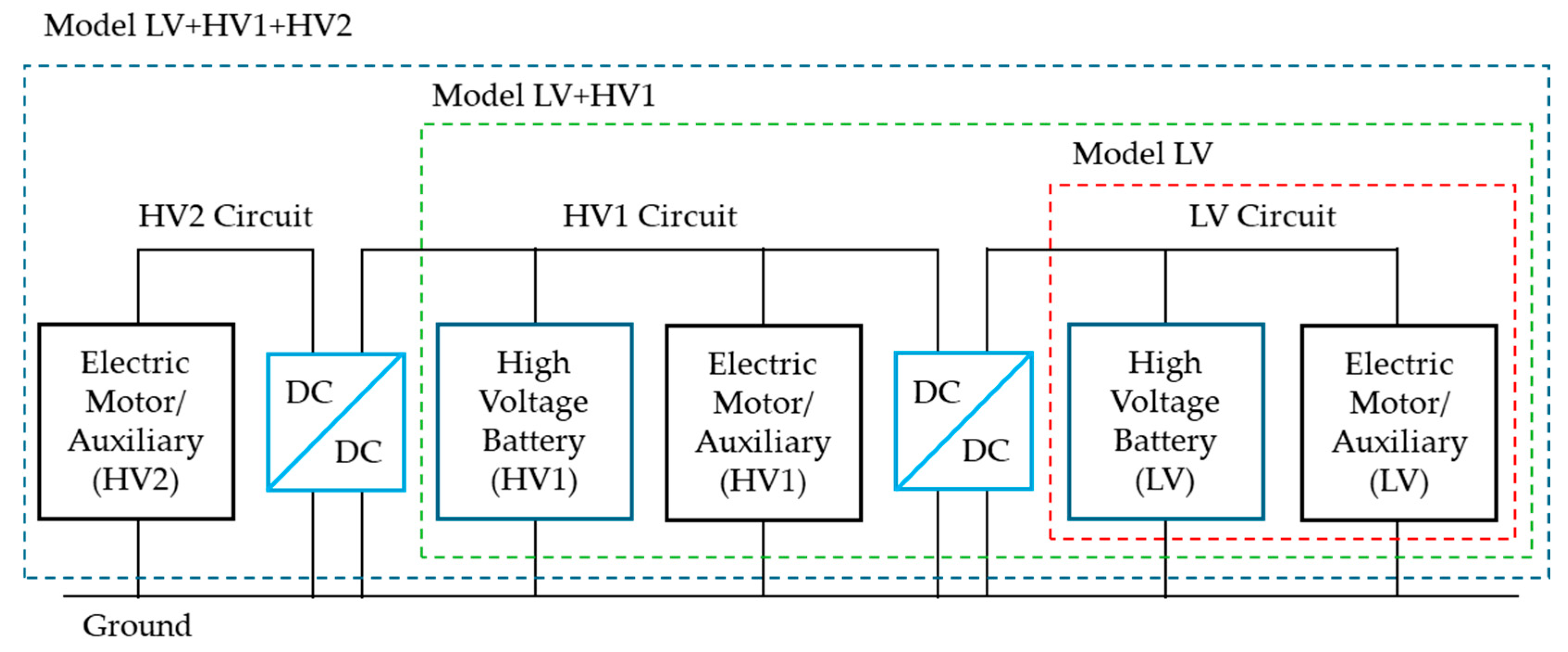
• Electric energy management for controlling battery State-of-Charge (SoC) and Depth-of-Discharge (DoD);
• Estimate the maximum torque of the electric generator at each rotation;
• Calculate the maximum quantity of energy used to power HV electric motors and other LV electric consumers in the vehicle’s system.

The electric energy flux from batteries to electric consumers is modeled using power consumption equations, which are generated by high-tension consumers P_HV and low-tension consumers P_LV [37,38].

$$P_{HV}=P_{AuxHV}+{\sum }_i{P}_{MotorHV}+{\displaystyle \frac{P_{HVtoLV}}{{\eta }_{DC-DC}}} \mathrm{for} P_{HVtoLV}\ge 0$$

(4)

$$P_{HV}=P_{AuxHV}+{\sum }_i{P}_{MotorHV}+P_{HVtoLV}·{\eta }_{DC-DC} \mathrm{for} P_{HVtoLV}<0$$

(5)

$$P_{LV}=P_{AuxLV}+\sum _i{P}_{MotorLV}-P_{HVtoLV}$$

(6)

where P_AuxHV and P_AuxLV represent the power consumed by electric auxiliary devices, P_MotorHV and P_MotorLV represent the power generated by each electric motor in the vehicle’s architecture, P_HVtoLV represents the power consumed by the DC-DC converter, and η_DC-DC represents the DC-DC converter’s voltage.

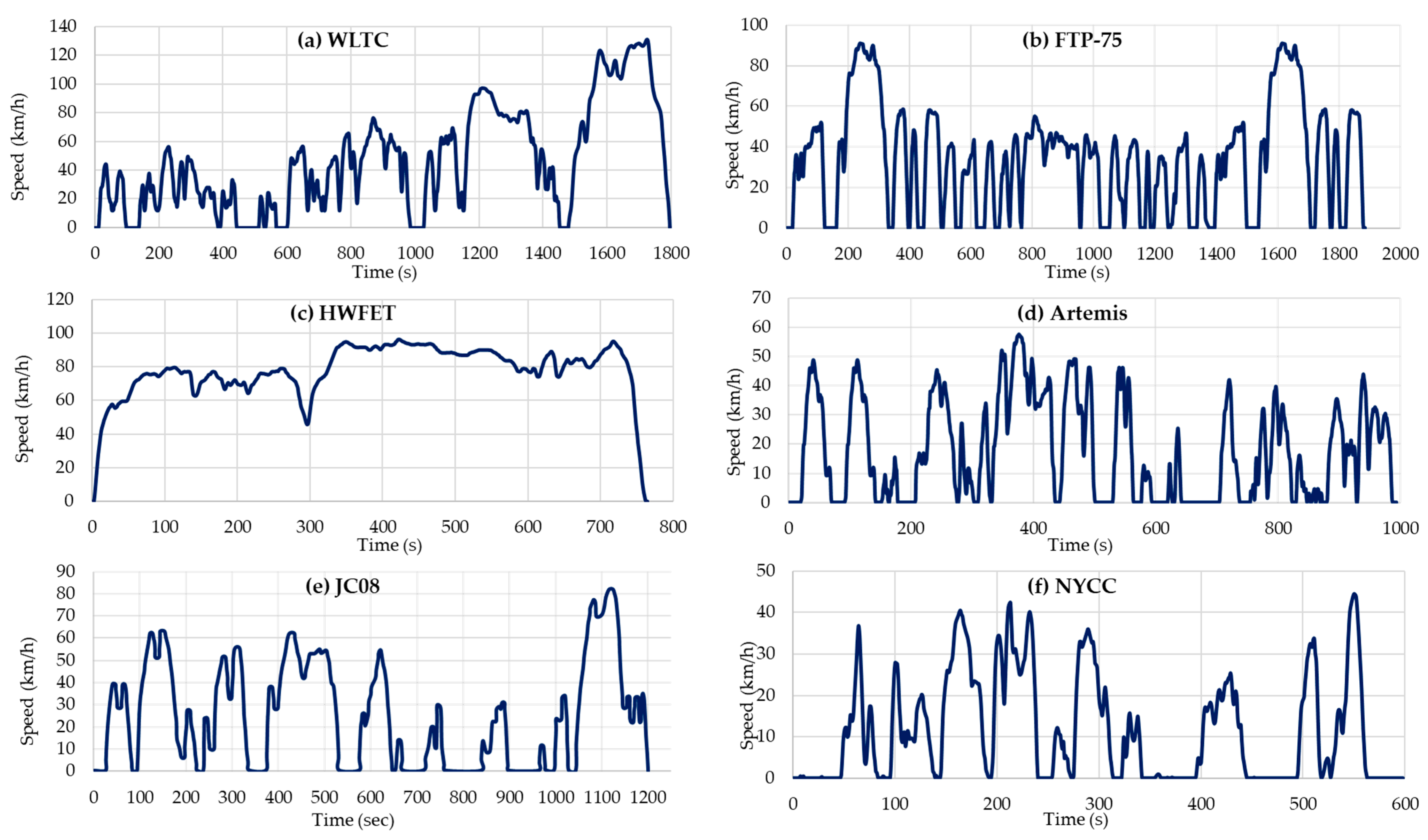
2.3.2. Virtual Model for Simulation Cycle

The driving cycles (Figure 6) that were selected for computer simulations were implemented and validated in the CarMaker (version 12) application developed by the company IPG Automotive (Karlsruhe, Germany) [38]. These are part of the manufacturer’s validated element library (IPG Automotive) and are available to licensed users.

The main characteristics of the driving cycles considered as they were implemented in driving scenarios from CarMaker/Scenario Editor/Maneuver are presented in

Table 3. Driving cycle characteristics as integrated into CarMaker/Scenario Editor/Maneuver.

Parameters	WLTC	FTP-75	HWFET	ARTEMIS	JC08	NYCC
Distance (m)	23,266	17,769	16,503	4874	8159	1902
Duration (s)	1800	1877	765	993	1204	598
Maximum speed (km/h)	131.30	91.25	96.32	57.32	81.60	44.45
Average cycle speed (km/h)	46.53	34.08	77.70	17.70	24.40	11.50
Average driving speed (km/h)	53.21	41.57	77.76	22.29	34.24	16.63
Driving time (s)	1574	1539	759	787	858	412
Maximum acceleration (m/s2)	1.67	1.48	1.43	2.86	1.69	2.68
Average acceleration (m/s2)	0.41	0.51	0.20	0.53	0.43	0.00
Minimum deceleration (m/s2)	−1.50	−1.48	−1.48	−1.48	−1.22	−1.50
Average deceleration (m/s2)	−0.45	−0.58	−0.22	−0.57	−0.46	−0.48
Standing time (s)	226	338	1	206	346	186
Number of stops (-)	8	19	1	14	11	7

[45].

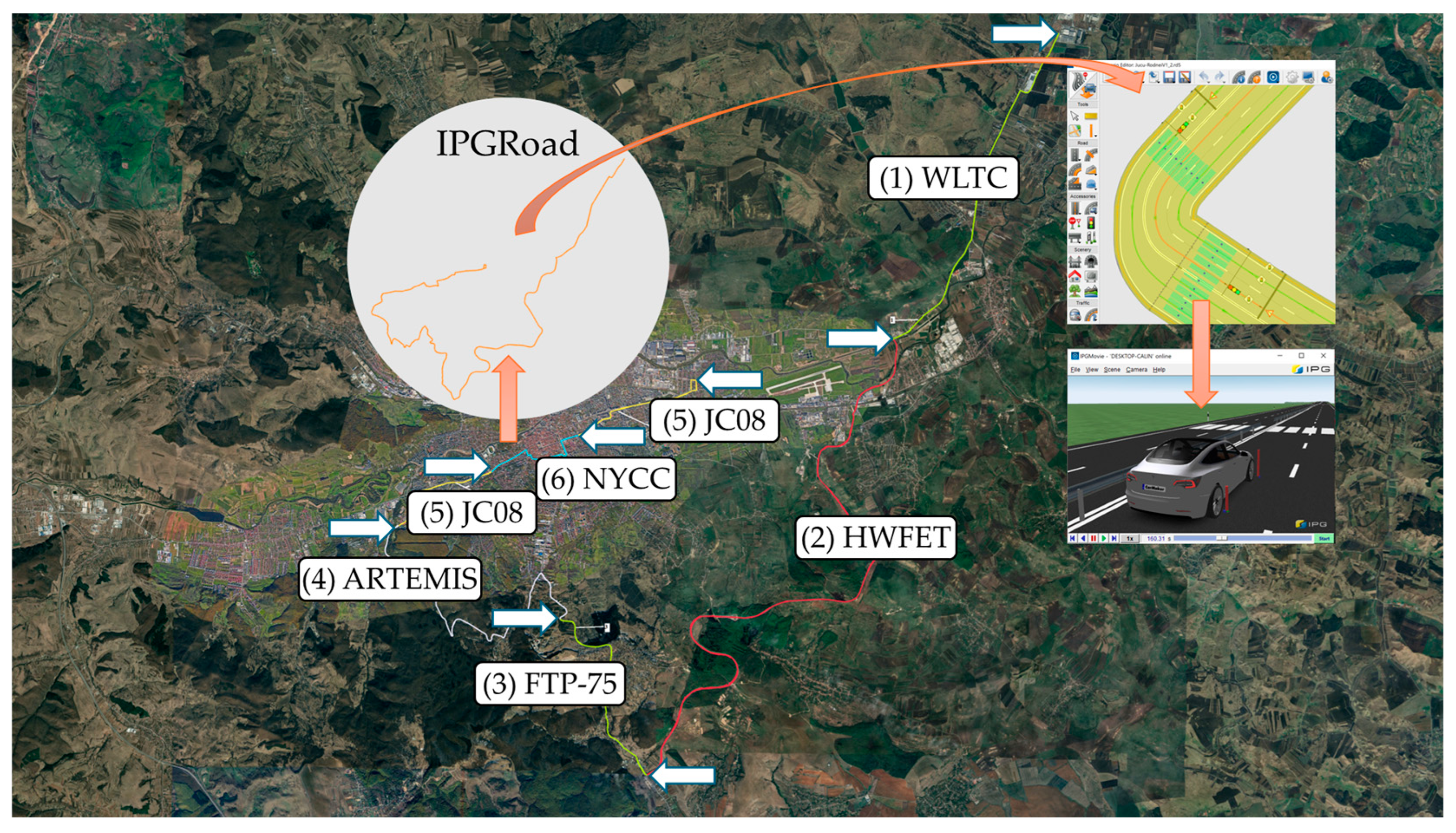
2.3.3. Virtual Road for Metropolitan Area

The selected route to perform computer simulations was created in CarMaker/IPGRoad (Figure 7), starting with the route used for experimental determinations with the Tesla Model 3. This route covers the metropolitan area of Cluj, Romania, on one of the most heavily trafficked sections of the main road, including the center area on the west axis and the ring road for accessing the industrial zone from the north to the south via the Transylvania Highway [46].

Similarly to the case presented, Magosi et al. in [47] developed virtual models for roads used in computer simulations, with an infrastructure consisting of the following elements: traffic lights, traffic lines, road markings, borders, barriers, traffic signs, public lighting, and more.

2.3.4. Virtual Environment

The detailed description of the environment allows for the smallest possible difference between the real scene and the virtual reality. Thorat et al. used the virtual environment model in [48], which was developed based on a virtual road model, an infrastructure model, and a weather model. The model in discussion is based on real-world road maps that have been digitized using geographic coordinates from Google Maps. For a photorealistic visualization of 3D scenes, the authors used CarMaker/Movie NX. This equipment uses physical rendering through 3D processing to ensure a combination of realistic illumination and meteorological effects appropriate for each simulation scenario [49].

Meteorological conditions were established in the CarMaker/Virtual Environment utility for computer simulations using data from the Raspisaniye Pogodi meteorological station [50], which provides real-time data, including a meteorological archive with complete data records from recent years. The extra time interval (date/time) from the meteorological archive was corresponding to the displacement in real traffic conditions with the Tesla Model 3 on the road considered for the acquisition of experimental data.

The mathematical model for the environment is defined based on equations that specify air temperature, air pressure, air density, and sound speed [37]. The air temperature in the ambient environment is calculated using the following equation [37,38]:

$$T=T_0+T_{elev}+T_{sRoad}+T_{time}$$

(7)

where T₀ is the temperature for height above mean sea level zero, T_elev is the temperature compensation factor based on elevation, T_sRoad is the temperature compensation factor based on road coordinates, and T_time is the temperature compensation factor based on time of day.

The temperature of the air as a function of elevation is calculated using the following equation [37,38]:

$$T_{elev}=∆h·C_{elev}$$

(8)

where Δh is the difference in height above the mean sea level and C_elev is the temperature decrease coefficient.

The ambient air pressure is calculated using the following equation [37,38]:

$$p=p_0{\left(1+{\displaystyle \frac{\Delta h·C_{elev}}{T_0}}\right)}^{5.255}$$

(9)

where p₀ is the pressure for height above the mean sea level zero.

The density of air in the ambient environment is calculated using the following equation [37,38]:

$$\rho ={\displaystyle \frac{\mathrm{p}}{R_s·T}}$$

(10)

where R_s is the specific gas constant.

The speed of sound in the air is calculated using the following equation [35,36]:

$$C_s=\sqrt{k·T·R_s}$$

(11)

where k is the air’s heat capacity ratio.

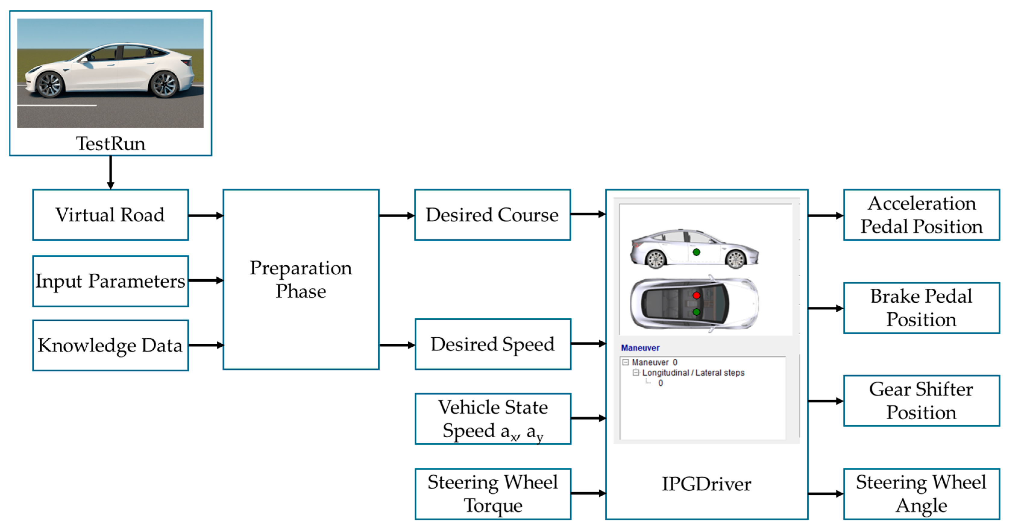
2.3.5. Virtual Driver Behavior

The ideal virtual driver behavior for computer simulations is based on Tesla’s Autopilot features [31].

The evaluated Tesla Model 3 is equipped with Autopilot hardware [27] that assists the driver and provides intuitive access to travel information, with the driver in charge of controlling the vehicle’s movement. According to SAE J3016™ [51], Tesla’s Autopilot system is classified as LEVEL 2^TM (partial automation) [52], with the driver’s role being to assist with Dynamic Driving Tasks (DDTs) during critical situations. Driving is continuously monitored, with the driver’s gaze fixed on the road (eyes on), and the driver’s hands can be temporarily removed from the wheel of the vehicle (hands temp off) [53].

The Autopilot system, based on the information provided by the video camera set, which is equipped with a real-world vehicle model and radar sensors to match up with the virtual vehicle model, provides the following ADAS driving assistance functions [54]:

• Traffic-Aware Cruise Control is a function that allows for adaptive cruise control in response to vehicles in front of it;
• Autosteer is a function that allows for the maintaining of traffic lanes and the direction of movement while steering;
• Auto Lane Change—a function that allows for a vehicle to change lanes automatically using a direction indicator (on turn signal);
• Navigate on Autopilot—a feature that allows for the following of a predetermined route based on GPS coordinates;
• Autopark—a function that allows for parking parallel or perpendicular to the roadside;
• Actually Smart Summon is a function that allows the vehicle to be moved from its parking spot to the location where the driver has summoned it by a maximum of 6 m.

All these functions were defined and configured throughout the virtual model’s development using the CarMaker/IPGDriver application [38].

Endsley [54] determined that after traveling over 4300 km during a six-month period in a Tesla vehicle with the mentioned assistance functions, at least one of these functions was activated in 84% of the trips.

Simulating command and control actions of a real-world driver in IPGDriver is accomplished by providing input parameter values, calculating a response based on the virtual model’s operating algorithm, and transmitting output parameter values to the virtual propulsion and direction system (Figure 8) [38].

CarMaker was used to replicate driving behavior, including both conventional and extended driver presets. These presets determine longitudinal and lateral accelerations, and they include three main driving styles:

(1)

“Normal” driver characterized by moderate acceleration and braking typical of daily driving;

(2)

“Defensive” driver characterized by constant, anticipatory driving with lower peak loads and potentially better energetic efficiency;

(3)

“Aggressive” driver characterized by fast acceleration and late breaking, resulting in increased energy consumption and reduced regeneration rate.

Camera sensors that incorporate both the virtual and real models for the Tesla Model 3 are positioned to provide a circular image of the surrounding environment and belong under the category of Hi-Fi (High Fidelity) virtual sensors. Camera sensors filter sent information and add data about physical effects that occur in the real world, particularly in terms of object detection and classification. Camera sensor characteristics include the ability to detect visible objects for the sensor, estimate distances to visible objects, and calculate the height of objects (occlusion calculation) [37].

The detection of objects in close proximity is dependent on the environment parameters RainRate and VisRangeInFog. The visibility α_Env camera sensor is calculated using the following equation [37,38]:

$${\propto }_{Env}=\mathrm{m}\mathrm{a}\mathrm{x}(1.0-{\displaystyle \frac{RainRate}{{RainRate}_{max}}},0)·\left({\displaystyle \frac{VisRangeInFog}{{VisRange}_{max}}},1\right)$$

(12)

where RainRate_max and VisRange_max are maximum values for environmental parameters.

Distance estimation Dist_Est to visible objects is calculated using the following equation [37,38]:

$${Dist}_{Est}={\displaystyle \frac{{Dist}^2}{f·b}}·{Dist}_{Err}$$

(13)

where Dist is the actual distance to the object, f is the camera’s focal length, b is the baseline, and Dist_Err is the disparity error.

The radar sensor that is equipped on the virtual model for the Tesla Model 3 corresponds to the RSI (Raw Signal Interface) sensor category, which provides raw information and functions similarly to real sensors. The CarMaker simulation application collects, filters, and interprets information transmitted by RSI Radar sensors, which complements the virtual model.

Radar sensor detection characteristics are based on the Signal-to-Noise Ratio (SNR), taking into account the following: detection threshold, antenna gain characteristics, transverse radar cross-sections (RCSs) of detected objects, propagation characteristics in relation to atmospheric conditions, and object occlusion [37].

The minimum detection threshold (SNR_min) is calculated using the following equation [37,38]:

$${SNR}_{min}=2{({erfc}^{-1}\left(2P_{FA}\right)-{erfc}^{-1}\left(2P_{Dmin}\right))}^2$$

(14)

where P_FA represents the probability of a false alarm, whereas PD_min is the least probability of detection.

The intensity of the received signal S_S is calculated using the following equation [37,38]:

$$S_s={\displaystyle \frac{P_{Radar}{G}_{Ant}^2{\lambda }^2\left(RCS\right)}{{\left(4\pi \right)}^3{r}^4}}·{\displaystyle \frac{1}{L_A{L}_{Atm}}}$$

(15)

where P_Radar is transmitted power, G_Ant is antenna gain, λ is wavelength, RCS is radar cross-section, r is the distance between the radar sensor and the monitored object, L_A denotes extra system losses, and L_Atm represents atmospheric losses.

The antenna gain is calculated based on the antenna direction (x, y, z) and the elevation θ and azimuth φ parameters, according to the following equation [37,38]:

$$f\left(\theta ,\phi \right)={\displaystyle \frac{\sin \left(\pi v_y\right)}{\left(\pi v_y\right)}}·{\displaystyle \frac{\sin \left(\pi v_z\right)}{\left(\pi v_z\right)}}={\displaystyle \frac{\sin \left(\pi \frac{a}{\lambda }\sin \theta \cos \phi \right)}{\left(\pi \frac{a}{\lambda }\sin \theta \cos \phi \right)}}·{\displaystyle \frac{\sin \left(\pi \frac{b}{\lambda }\sin \theta \cos \phi \right)}{\left(\pi \frac{b}{\lambda }\sin \theta \cos \phi \right)}}$$

(16)

where parameters a and b represent the primary lobe of the aperture dimensions.

Transversal RCS thresholds for objects within close proximity are determined by radar sensor resolution, object size, direction of incidence, object occlusion, and object merging (Figure 9).

The Autopilot functions that equip the Tesla Model 3 have been implemented in the virtual model via the Vehicle Control module, where there are two models of autonomous driving functions: GLxC (Generic Longitudinal Control) for vehicle movement (

Table 4. Model GLxC (Generic Longitudinal Control) for vehicle movement.

Parameters	Unit	Value
Autonomous emergency braking
Referenced object sensor	-	Front radar
Maximal deceleration	m/s2	6.0
Acceleration controller factor P (proportional)	-	0.001
Acceleration controller factor I (integral)	-	3.0
Minimal distance	m	5.0
Time braking after standstill	s	5.0
Time brake reacts	s	0.2
Forward collision warming
Time first warming level	s	2.0
Time second warming level	s	1.0

) and GLyC (Generic Lateral Control) for vehicle direction (

Table 5. Model GLyC (Generic Lateral Control) for vehicle direction.

Parameters	Unit	Value
Initial line detection mode	-	Line sensor
Line keeping assist system
Maximal velocity	km/h	55.0
Maximal assist torque	Nm	2.0
Time constant PT (powertrain) filter	s	0.003
Maximal lane width	m	7.0
Minimal line width	m	1.8
Curvature controller factor P (proportional)	-	2.0
Curvature controller factor I (integral)	-	0.2
Curvature controller factor D (derivative)	-	0.0
Maximal deviation distance	m	10.0
Assist torque coefficient	Ns2	2.0
Lane departure warning
Maximal velocity	km/h	55.0
Distance departure warning	m	0.2

).

Trajectory planner (TP) for virtual model movement has been implemented based on a set of established rules for planned routes with well-defined boundaries. The rule set can determine whether the vehicle remains on the current travel lane or should change lanes. A travel scenario assumes that the virtual vehicle model is placed in the middle of the right-hand lane. If a slower vehicle moves in front of the virtual model, preventing it from reaching stable cruising speed, and the lane on the left is free, a Bézier curve is planned to change the lane of circulation [55].

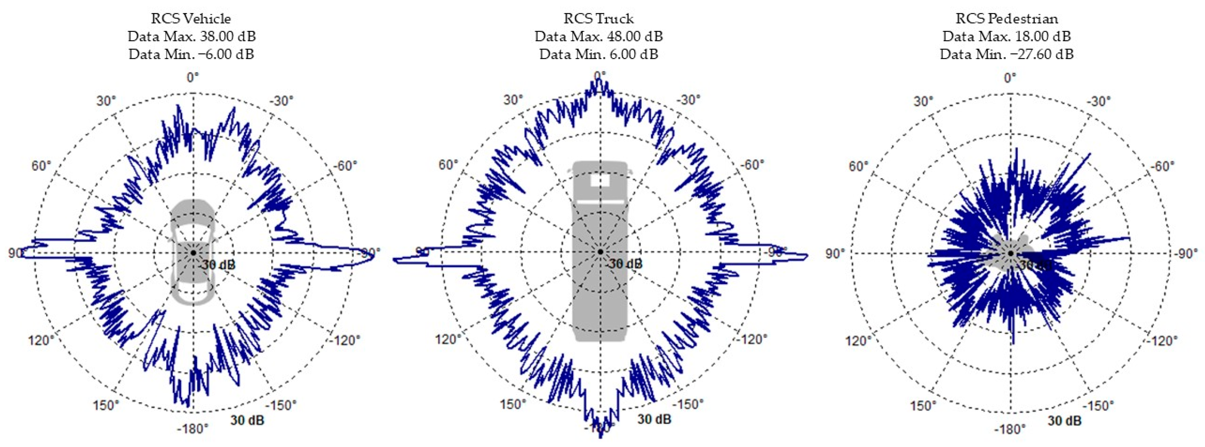
2.3.6. Virtual Traffic Model

The virtual traffic model includes a set of maneuvers to move traffic-related movable objects. Each maneuver consists of a longitudinal and a lateral component [31].

To simulate a random/stochastic traffic model for urban and metropolitan areas, the following scenarios were generated: static vehicles, slow-driving vehicles, fast-driving vehicles, vehicles that abruptly change lanes, vehicles that coincide at a crossing, bicycle riders, and pedestrians crossing the road [22].

Noei et al. [56] used CarMaker simulation tools to evaluate vehicle tracking behaviors, change driving lane, and adapt movement for the simulation of driving scenarios in a generated traffic environment. As a result, the virtual traffic model includes ten different types of drivers (from conservative to aggressive), ten different vehicle models, various driving scenarios, potentially dangerous interventions from other traffic participants, and other unknown situations.

The virtual traffic model was considered for governing computer-generated road simulations implemented in CarMaker/Road. In the computer simulations for which the cycles of movement described in Section 2.3.2 “Virtual Model for Simulation Cycle” were implemented, the virtual traffic model was not used; it was instead replaced by procedures for controlling the driving cycles (acceleration/deceleration).

2.4. Driver-in-the-Loop Simulator

2.4.1. Simulator Development

The existing literature has mainly utilized standardized driving cycles and simulation platforms like CarMaker to assess electric vehicle energy use. However, a few research studies have successfully merged virtual vehicle modeling, real-world driving data, and driver behavior variability in a validated simulation context. In particular, the ability of Driver-in-the-Loop systems to bridge the gap between theoretical models and actual driving behavior has been undervalued.

Driving simulators based on virtual vehicle models have been used in studies and by other research groups. As a result, Kwon et al. [57] used a compact driving simulator that included real-world vehicle components to assess driving behaviors for different drivers in laboratory conditions.

Aparow et al. [58] used a driver-in-the-simulation platform to verify and validate the simulation model developed in Matlab Simulink and CarMaker based on various test scenarios, defined with real traffic data.

The virtual scenarios described in previous chapters have been implemented in a simulator built on the Driver-in-the-Loop simulator concept (Figure 10) [59,60,61], which is used to run computerized simulations based on real-world scenarios traveled by the Tesla Model 3 on the selected road.

CarMaker/CockpitPackage extension permits controlling the movement of a virtual vehicle using an external control device, which in our case is a Logitech G Driving Force G920 Wheel [22].

The CockpitPackage software (version 12) architecture is based on a multiplatform development library called SDL2 (Simple Direct-media Layer), and simulator input signals are divided into the following two categories:

• Axis events indicate the evolution of movement on coordinate axis, which are analogic values generated by the steering wheel and/or pedal actions;
• Button events are actions that correspond to “true” or “false” values for certain predetermined selections, like light blocks, signalization, and sound alerts.

2.4.2. Simulation Task

Using the virtual Tesla Model 3 model, computer simulations were run for the following tasks under similar environmental and traffic conditions to those used for experimental data collection in the considered metropolitan area:

• In CarMaker with the plug-in Cockpit Package Standard, a human driver used a virtual Tesla Model 3 to simulate real-world driving conditions using a Driver-in-the-Loop simulator. The following parameters were monitored and recorded using CarMaker/IPGControl: Car.Distance (m), speed (km/h), consumption, respective recovery of electric energy PT.BattHV.Energy (kWh), and the key parameters of SoC battery charging PT.BCU.BattHV.SOC (%).
• ADAS functions (according to Level 2 SAE 3016^TM) [51] ran computer simulations using a virtual Tesla Model 3 model similar to real driving conditions, ensuring movement control through the CarMaker/IPGDriver utility in standard driver mode in accordance with the values of the parameters corresponding to the behavioral profile of the virtual driver presented in

  Table 6. Characteristic parameters for standard driving mode.

  Standard Driving Mode	Longitudinal Acceleration (m/s2)	Longitudinal Deceleration (m/s2)	Lateral Acceleration (m/s2)
  Driver presets standard “Normal”	3.00	−4.00	4.00
  Driver presets standard “Defensive”	2.00	−2.00	3.00
  Driver presets standard “Aggressive”	4.00	−6.00	5.00

  in extended driver mode in accordance with the values of the parameters corresponding to the behavioral profile of the virtual driver presented in

  Table 7. Characteristic parameters for extended driver driving mode.

  Extended Driver Driving Mode	Dynamics	Energy Efficiency	Nervousness
  Energy-efficient driver	0.20	0.10	0.00
  Stressed driver	0.70	0.00	0.50

  . These profiles have been created to represent realistic behavioral differences and to evaluate fuel economy under a variety of scenarios. The “Normal” driver profile represents most drivers’ average daily driving and achieves a balance trade-off, with the maximum regeneration rates found during WLTC and FTP-75 driving cycles. The “Defensive” driver profile illustrates careful driving with smoother acceleration–braking transitions, which decreases energy consumption while simultaneously reducing regeneration events due to smoother deceleration. The “Aggressive” driver profile illustrates impulsive behavior with rapid acceleration and late braking, which repeatedly results in increased energy consumption and low regeneration caused by abrupt braking.

The integration of real-world driving scenarios into a digital world of computer simulations is a critical step in the research and development of modern vehicles. To implement these scenarios as accurately as possible, various vehicle driving cycles have been used, which reflect the behavior of a driver in a variety of driving situations, such as variable traffic, urban, and extra-urban [62].

The workflow for the calibration–validation of the virtual model and computer simulations included the following steps:

(1) Vehicle data acquisition: Experimental data (energy consumption, energy recovery rates, and speed profiles) were collected while driving in real-world situations in predefined metropolitan sectors.

(2) Virtual vehicle modeling: The structural and behavioral parameters of the Tesla Model 3 were implemented in CarMaker using manufacturer-provided data.

(3) Reference simulation: The following driving cycles (WLTC, FTP-75, HWFET, ARTEMIS, JC08, and NYCC) were performed initially without behavioral calibration.

(3a) Simulation calibration requires iterative adjustments to simulation parameters like the driver behavioral profile (“Normal”, “Defensive”, and “Aggressive”), the environment conditions, and the powertrain settings.

(3b) To validate the simulation, we compared the derived findings to the experimental data using RMSE (Root Mean Square Error), MAPE (Mean Absolute Percentage Error), and 95% confidence intervals.

(4) A stopping criterion for calibration iterations was used when the MAE (Mean Absolute Error) between simulated and experimentally confirmed total energy consumption in all sectors traveled was <5%.

3. Results

3.1. Experimental Results

The route selected for a journey with a Tesla Model 3 in the Cluj metropolitan area has been divided into sections based on the city of Cluj-Napoca’s zonal boundaries. The route is divided into five main segments, with each sector considered in the order in which the vehicle was driven for experimental data collection.

The experimental results were derived from real-world consumption graphs of the Tesla Model 3 and include information on the length of the road, the average speed of movement in each sector, the amount of energy consumed by the vehicle, and the amount of energy recovered through energy recovery (

Table 8. Experimental results in metropolitan area (real vehicle Testa Model 3).

Area	Length (m)	Average Speed (km/h)	Energy Consumption (kWh/km)	Recovered Energy (kWh/km)	Total Energy (kWh/km)
Extra-urban metropolitan 1	10,030	54.99	0.177	0.031	0.146
Metropolitan ring	20,020	81.30	0.269	0.023	0.269
Extra-urban metropolitan 2	5970	54.40	0.187	0.009	0.178
Urban metropolitan	10,240	42.00	0.172	0.029	0.143
Urban peripheral 1	3330	17.48	0.130	0.011	0.119
Urban central	3290	15.70	0.173	0.010	0.163
Urban peripheral 2	4460	21.00	0.179	0.016	0.163

). The energy values are calculated per kilometer. Energy recovery is based on regenerative braking events recorded in the vehicle’s ECU records.

The experimental results obtained after completing a selected real-world route in the metropolitan area have been utilized as a reference value in validating computer simulations with a virtual model for Tesla Model 3.

CarMaker/Environment and CarMaker/Load utilities were used to configure the medium and load parameters of the virtual model to make them similar to real-world conditions.

3.2. Simulation Results

All experimental data collected after completing the selected route in the Cluj metropolitan area were compared to the results obtained with the virtual Tesla Model 3 after running simulations in CarMaker on the Driver-in-the-Loop simulator for the metropolitan route (

Table 9. Simulation results in metropolitan area (virtual model Tesla Model 3 on Driver-in-the-Loop simulator).

Area	Length (m)	Average Speed (km/h)	Energy Consumption (kWh/km)	Recovered Energy (kWh/km)	Total Energy (kWh/km)
Extra-urban metropolitan 1	10,035	54.99	0.170	0.020	0.150
Metropolitan ring	20,020	81.30	0.220	0.025	0.195
Extra-urban metropolitan 2	5970	54.40	0.180	0.010	0.170
Urban metropolitan	10,240	42.00	0.165	0.030	0.135
Urban peripheral 1	3330	17.48	0.125	0.015	0.110
Urban central	3290	15.70	0.160	0.010	0.150
Urban peripheral 2	4460	21.00	0.170	0.020	0.150

), respectively, for selected and implemented driving cycles on the corresponding sectors based on driving cycle characteristics (

Table 10. Simulation results in Metropolitan area (virtual model Tesla Model 3 on driving cycles).

Driving Cycle	Cycle Length (m)	“Normal” Driving Behavior			“Aggressive” Driving Behavior			“Defensive” Driving Behavior
		Average Speed (km/h)	Energy Consumption (kWh/km)	Energy Recovered (kWh/km)	Average Speed (km/h)	Energy Consumption (kWh/km)	Energy Recovered (kWh/km)	Average Speed (km/h)	Energy Consumption (kWh/km)	Energy Recovered (kWh/km)
(1) WLTC	23,266	46.13	0.188	0.040	46.07	0.201	0.000	40.32	0.173	0.005
(2) HWFET	16,503	77.67	0.166	0.023	77.54	0.173	0.000	72.38	0.155	0.018
(3) FTP-75	17,769	34.11	0.162	0.014	34.07	0.169	0.000	30.99	0.150	0.006
(4) ARTEMIS	51,687	17.63	0.183	0.003	17.60	0.256	0.000	15.66	0.163	0.002
(5) JC08	8159	24.42	0.174	0.003	24.39	0.194	0.000	21.93	0.145	0.002
(6) NYCC	1902	11.38	0.216	0.002	11.34	0.235	0.000	9.57	0.198	0.002

).

The average speed (km/h) was calculated based on the distance traveled on each road sector and the time needed to complete these sectors.

The energy consumption (kWh/km) in each sector is influenced by travel speed, the structure of the road, and traffic conditions. Because real traffic could not be implemented identically in the simulating process, in the initial conditions for defining simulating tasks, speed was maintained constantly for each sector and considered to be the medium speed required to complete the sector.

The recovered energy (km/h) from regenerative braking was determined from the graphic recorded in the ECU of the Tesla Model 3 and was taken into consideration in computerized simulations of each road sector by defining some braking actions in the CarMaker/Maneuver tool.

As mentioned in Section 2.3.6 “Virtual traffic model” for each of the sectors considered, one of the driving cycles available in the CarMaker library was chosen and implemented. The association of selected driving cycles to road sectors was accomplished by considering the vehicle’s operational model and travel regime in relation to traffic characteristics and by considering the respective speed limits for the sectors under consideration.

For virtual traffic model simulation in urban zones (urban center, urban peripheral 1, urban peripheral 2), driving cycles like JC08, NYCC, and ARTEMIS were considered, which assume a low average travel speed with frequent acceleration and deceleration.

On routes from urban metropolitan zones (urban metropolitan, extra-urban metropolitan 1, and extra-urban metropolitan 2), which are generally located adjacent to major urban agglomerations and are crossed by national road with speed restrictions, universal driving cycles WLTC and FTP-75 have been selected.

The highway driving cycle (HWFET) has been chosen for sections of the metropolitan ring where traffic moves at a high speed in a relatively steady flow of vehicles.

To cover all types of driver behavior, computer simulations for each sector were evaluated with core sets in CarMaker/Driver for three characteristics of the driver behavior: “Normal” driver behavior, “Aggressive” driver behavior, and “Defensive” driver behavior (Table 10).

The virtual model was evaluated using six globally recognized driving cycles. To validate the virtual model and the results, the simulation’s accuracy was verified using RMSE, MAPE, and set confidence intervals (

Table 11. Evaluating simulation accuracy with statistical error metrics.

Area	RMSE (kWh/km)	MAPE (%)	Confidence Interval (kWh/km)
Extra-urban metropolitan 1	0.019	3.45	0.130–0.150
Extra-urban metropolitan 2
Metropolitan ring	0.015	3.87	0.138–0.155
Urban metropolitan	0.017	4.21	0.149–0.167
Urban central	0.013	7.98	0.140–0.160
Urban peripheral 1	0.011	4.61	0.124–0.140
Urban peripheral 2
Average for all sectors	0.016	4.52	-

). The results provide both theoretical insights and useful recommendations for enhancing the energy efficiency of electric vehicles in a variety of driving scenarios.

Figure 11a–f display the graphs for energy consumed and energy recovered for each of the driving cycles selected for the sectors under consideration.

The operating conditions for driving cycles (see Table 3) involve frequent and significant acceleration, which determines the consumption of additional electric energy from the electric motor to generate the necessary power for motion. The energy balance for total electric energy consumption E includes the quantity of energy consumed C during acceleration and the quantity of energy recovered R during deceleration.

$$E\left(x\right)=\sum _{i=1}^n{C}_i\left(x\right)+\sum _{j=1}^m{R}_j\left(x\right)$$

(17)

where x represents the driving cycles $x\in (a-f)$, n represents the number of accelerations that determine the energy consumption, and m represents the number of decelerations that determine the energy recovery.

The recovery of energy in the graphs in Figure 11 is highlighted by a constant level, which can represent a growing trend in the evolution of energy consumption in the graph sections that follow a significant deceleration.

In circumstances in which the deceleration is excessive, mechanical braking is activated without the recovery of energy. Similarly, excessive acceleration increases the instantaneous power demand of the electric motor, resulting in a significant increase in electric energy consumption and a decrease in autonomy. Similarly, strong braking sequences reduce energy recovery efficiency, resulting in increased energy consumption and decreased autonomy [63].

4. Discussions

To evaluate electric energy consumption in the driving scenarios considered in metropolitan areas, evaluations have been implemented in a virtual model simulating the six variants of driving cycles assimilated to sectors that have travel conditions similar to these driving cycles’ characteristics (Figure 12).

Extra-urban metropolitan 1 (17.49% of total route) and extra-urban metropolitan 2 (10.41% of total travel) have been integrated into the WLTC driving cycle, which tests the performance of vehicles in circulation under all conditions. Under WLTC, moderate and repetitive decelerations maximize regenerative braking during “Normal” driving, whereas the same cycle under defensive driving requires sufficient kinetic energy dissipation to trigger effective regeneration.

The metropolitan ring (34.91% of the total route) that provides rapid transportation on the ring road with a medium to high speed (up to 80 km/h) has been integrated into the HWFET driving cycle, which tests the performance of vehicles on highway driving conditions. The HWFET allows for more stable operation, which reduces total energy consumption due to fewer transient intervals while simultaneously reducing regenerative braking due to shorter breaking or deceleration intervals.

The FTP-75 cycle, which tests the performance of vehicles in circulation in all conditions of travel in the United States, has been incorporated into the urban metropolitan area (17.85% of the total route), which ensures constant travel at a medium speed of up to 42 km/h. By implementing this driving cycle in an area near an extra-urban metropolitan area, a comparison of the WLTC and FTP-75 results was performed.

Urban peripheral 1 (5.83% of the total route) allows for travel in variable traffic conditions to the periphery of the main city with a travel speed of up to 18 km/h. The ARTEMIS driving cycle, which investigates vehicle behavior in realistic urban traffic circumstances, has been incorporated into the simulation framework to improve energy efficiency predictions. This driving cycle produces abrupt kinetic changes, boosting the potential for energy recovery, as long as the deceleration happens within the regenerative braking window.

Urban central (5.73% of total route) provides urban mobility in the central areas of the settlement with a medium speed of up to 15 km/h. The NYCC driving cycle has been simulated, which tests the performance of vehicles in heavy traffic from urban agglomerations. Under NYCC, high stop frequency contributes to energy spikes, with aggressive behavior sharply penalizing efficiency. Regeneration efficiency correlates strongly with motor efficiency zones and the frequency/strength of deceleration events.

Urban peripheral 2 (7.78% of the total route) allows for variable traffic conditions at the local perimeter with a maximum travel speed of 21 km/h. The JC08 driving cycle is used to evaluate the performance of vehicles in urban traffic. During the implementation of this driving cycle in a nearby urban peripheral zone, a comparison of the results obtained with ARTEMIS and JC08 was performed.

Table 12. Energy consumption for the considered driving cycles.

Area	Total Energy Consumed						Total Energy Recovered
	(kWh/km)			(%) of Total			(kWh/km)			(%) of Total
	N	D	A	N	D	A	N	D	A	N	D	A
Extra-urban metropolitan 1, 2 (WLTC)	3.008	2.768	3.216	32.27	30.47	29.50	0.640	0.080	0.000	50.29	15.26	0.00
Metropolitan ring (HWFET)	3.320	3.100	3.460	35.62	34.16	31.77	0.460	0.360	0.000	36.18	68.77	0.00
Urban metropolitan (FTP-75)	1.650	1.530	1.730	17.79	16.90	15.87	0.143	0.060	0.000	11.28	11.72	0.00
Urban peripheral 1 (ARTEMIS)	0.400	0.540	0.850	4.39	5.97	7.82	0.009	0.006	0.000	0.78	1.27	0.00
Urban central (NYCC)	0.140	0.480	0.780	1.55	5.36	7.09	0.009	0.006	0.000	0.77	1.25	0.00
Urban peripheral 2 (JC08)	0.770	0.640	0.860	8.32	7.14	7.95	0.008	0.008	0.000	0.70	1.73	0.00

Note: N—“Normal”; D—“Defensive”; A—“Aggressive”.

shows the total quantity of energy consumed and recovered in the investigated areas for the three driver behavioral types evaluated (“Normal”, “Defensive”, and “Aggressive”).

The simulation results indicate that “Normal” driving behavior frequently results in higher energy regeneration than the “Defensive” or “Aggressive” profiles. This is because “Normal” driving requires more modest decelerations at speeds when the regenerative braking system is most effective. In contrast, “Aggressive” driving depends more on mechanical breaking (due to fast stops), but “Defensive” driving avoids deceleration rates that are sufficient to result in significant energy recovery.

The torque–speed efficiency curve (see Figure 3) of electric motors indicates that optimal regeneration occurs in a specific range of engine torque. “Aggressive” driving frequently exits this efficiency range prematurely, but “Defensive” driving rarely achieves it with sufficient intensity.

We compared our findings to previous research benchmarks, including the US Department of Energy baseline for EV urban consumption [29,30] (~0.18–0.22 kWh/km). Our results were within the expected limitations, supporting the simulation framework.

5. Conclusions

Electric vehicles have become an essential component of sustainable urban mobility. Their adoption has numerous advantages, including lower GHG emissions, lower noise pollution, and less reliance on fossil fuels. Beyond environmental benefits, electric vehicles have less expensive long-term operating costs due to enhanced drivetrain efficiency and simplified maintenance requirements.

However, the significant integration of electric vehicles into metropolitan infrastructure creates new issues, such as the requirement for sustainable charging networks, increased grid demand, and vehicle performance optimization under changing driving conditions. Understanding and predicting electric vehicle energy efficiency in real-world situations becomes increasingly important as cities transition to smart and sustainable ecosystems.

This study developed and evaluated a comprehensive simulation framework for evaluating the energy efficiency of electric vehicles in urban and metropolitan areas. Using CarMaker, a detailed virtual model of the Tesla Model 3 was calibrated using real-world driving data acquired in Cluj-Napoca, Romania, and tested during six standardized driving cycles. This work differentiates itself from previous studies that depend only on idealized cycle testing by using Driver-in-the-Loop simulation, multiple driver behavior profiles (“Normal”, “Defensive”, and “Aggressive”), and real-world traffic scenarios.

Environmental factors, virtual routes, driver behavior, and traffic scenarios were all considered when developing and validating the virtual model for the considered electric vehicle. These parameters reflect the technical and empirical distinctions that exist in real-world settings. The results from the simulations were extensively analyzed, and iterative optimization of the virtual models was performed until the simulation results exceeded those obtained from the experiments.

The final validated virtual model contributed to the certification of energy efficiency indicators by incorporating real-world driving data and behavior parameters. The virtual model was specifically calibrated for the Tesla Model 3 electric vehicle throughout a variety of urban and metropolitan traffic scenarios. These simulations were run under environmental and traffic circumstances similar to those discovered during empirical data collecting in the selected metropolitan area.

The merging of real-world driving scenarios into virtual simulation settings represents a significant step forward in the research and development of modern vehicles.

Our work provides significant contributions in the following areas:

(1)

A validated simulation workflow with quantitative calibration metrics (RMSE, MAPE, confidence intervals) achieved an average MAPE of 4.52% compared to experimental data.

(2)

A detailed analysis of how driving behavior affects energy consumption and regenerative efficiency, revealing nonlinear and sometimes unexpected trends.

(3)

Integrating real-world environmental and behavioral characteristics into a controlled simulation environment to improve the virtual model’s realism and reproducibility.

The main limitations of the current study include the following:

(1)

The structural architecture of the virtual model and the electric battery model cannot be generalized and are difficult to modify for other vehicle models;

(2)

While various driving scenarios were modeled, completely stochastic traffic environments and random vehicle interactions were simplified in the simulation process or replaced with mobility scenarios controlled by driving cycles;

(3)

The analysis of energy regeneration following regenerative braking focused on deceleration dynamics; the simulation process did not take into account thermal effects, the battery degradation process, and long-term performance deviation.

Future work will include the following studies:

(1)

Expanding the virtual modeling and simulation methods to include multiple electric vehicle platforms and enabling comparisons between them.

(2)

Using machine learning models to replicate real-time versatility and customization of driver behavior and vehicle settings.

(3)

Using simulation results to simulate the appropriate placement of urban charging stations using consumption–recovery models to achieve optimal Vehicle-to-Grid (V2G) interaction planning.

References

1. Alanazi, F. Electric Vehicles: Benefits, Challenges, and Potential Solutions for Widespread Adaptation. Appl. Sci. 2023, 13, 6016. [Google Scholar] [CrossRef]
2. Tsoi, K.H.; Loo, B.P.; Li, X.; Zhang, K. The co-benefits of electric mobility in reducing traffic noise and chemical air pollution: Insights from a transit-oriented city. Environ. Int. 2023, 178, 108–116. [Google Scholar] [CrossRef] [PubMed]
3. The Role of Electric Mobility for Low Carbon and Sustainable Cities. Available online: https://unhabitat.org/sites/default/files/2022/05/the_role_of_electric_mobility_for_low-carbon_and_sustainable_cities_1.pdf (accessed on 11 December 2024).
4. García-Vázquez, C.; Llorens-Iborra, F.; Fernández-Ramírez, L.; Sánchez-Sainz, H.; Jurado, F. Comparative study of dynamic wireless charging of electric vehicles in motorway, highway and urban stretches. Energy 2017, 137, 42–57. [Google Scholar] [CrossRef]
5. Muñoz-Villamizar, A.; Montoya-Torres, J.R.; Faulin, J. Impact of the use of electric vehicles in collaborative urban transport networks: A case study. Transp. Res. Part D Transp. Environ. 2017, 50, 40–54. [Google Scholar] [CrossRef]
6. Liang, J.; Feng, J.; Fang, Z.; Lu, Y.; Yin, G.; Mao, X. An Energy-Oriented Torque-Vector Control Framework for Distributed Drive Electric Vehicles. IEEE Trans. Transp. Electrif. J. 2023, 9, 4014–4031. [Google Scholar] [CrossRef]
7. Cavus, M.; Dissanayake, D.; Bell, M. Next Generation of Electric Vehicles: AI-Driven Approaches for Predictive Maintenance and Battery Management. Energies 2025, 18, 1041. [Google Scholar] [CrossRef]
8. Daouda, A.S.M.; Atila, Ü. A Hybrid Particle Swarm Optimization with Tabu Search for Optimizing Aid Distribution Route. Artif. Intell. Stud. (AIS) 2024, 7, 10–27. [Google Scholar] [CrossRef]
9. Aldossary, M. Enhancing Urban Electric Vehicle (EV) Fleet Management Efficiency in Smart Cities: A Predictive Hybrid Deep Learning Framework. Smart Cities 2024, 7, 3678–3704. [Google Scholar] [CrossRef]
10. Ran, X.; Suyaroj, N.; Tepsan, W.; Ma, J.; Zhou, X.; Deng, W. A hybrid genetic-fuzzy ant colony optimization algorithm for automatic K-means clustering in urban global positioning system. Eng. Appl. Artif. Intell. 2024, 137, 109237. [Google Scholar] [CrossRef]
11. Nguyen, T.H.; Jung, J.J. Ant colony optimization-based traffic routing with intersection negotiation for connected vehicles. Appl. Soft Comput. 2021, 112, 107828. [Google Scholar] [CrossRef]
12. Mirjalili, S.; Mirjalili, S.M.; Lewis, A. Grey Wolf Optimizer. Adv. Eng. Softw. 2014, 69, 46–61. [Google Scholar] [CrossRef]
13. Astarita, V.; Haghshenas, S.S.; Guido, G.; Vitale, A. Developing new hybrid grey wolf optimization-based artificial neural network for predicting road crash severity. Transp. Eng. 2023, 12, 100164. [Google Scholar] [CrossRef]
14. Nadimi-Shahraki, M.H.; Taghian, S.; Mirjalili, S. An improved grey wolf optimizer for solving engineering problems. Expert Syst. Appl. 2021, 166, 113917. [Google Scholar] [CrossRef]
15. Kar, A.K. Bio inspired computing—A review of algorithms and scope of applications. Expert Syst. Appl. 2024, 59, 20–32. [Google Scholar] [CrossRef]
16. Bazi, S.; Benzid, R.; Bazi, Y.; Al Rahhal, M.M. A Fast Firefly Algorithm for Function Optimization: Application to the Control of BLDC Motor. Sensors 2021, 21, 5267. [Google Scholar] [CrossRef]
17. Alshammari, N.F.; Samy, M.M.; Barakat, S. Comprehensive Analysis of Multi-Objective Optimization Algorithms for Sustainable Hybrid Electric Vehicle Charging Systems. Mathematics 2023, 11, 1741. [Google Scholar] [CrossRef]
18. Forcael, E.; Carriel, I.; Opazo-Vega, A.; Moreno, F.; Orozco, F.; Romo, R.; Agdas, D. Artificial Bee Colony Algorithm to Optimize the Safety Distance of Workers in Construction Projects. Mathematics 2024, 12, 2087. [Google Scholar] [CrossRef]
19. Iclodean, C.; Varga, B.O.; Cordos, N. Virtual Model. In Autonomous Vehicles for Public Transportation; Springer: Cham, Switzerland, 2022; pp. 195–335. [Google Scholar]
20. Release 14.0 CarMaker Product Family. Feature Highlights. Available online: https://www.ipg-automotive.com/en/products-solutions/software/highlights-carmaker-product-family (accessed on 17 December 2024).
21. Ricciardi, V.; Ivanov, V.; Dhaens, M.; Vandersmissen, V.; Geraerts, M.; Savitski, D.; Augsburg, K. Ride Blending Control for Electric Vehicles. World Electr. Veh. J. 2019, 10, 36. [Google Scholar] [CrossRef]
22. IPG Automotive. User’s Guide Version 12.0.3 CarMaker. In Solutions for Virtual Test Driving; IPG Automotive Group: Karlsruhe, Germany, 2024. [Google Scholar]
23. IPG Automotive. InfoFile Description Version 12.0.3 IPGRoad. In Solutions for Virtual Test Driving; IPG Automotive Group: Karlsruhe, Germany, 2024. [Google Scholar]
24. Toth, B.; Szalay, Z. Development and Functional Validation Method of the Scenario-in-the-Loop Simulation Control Model Using Co-Simulation Techniques. Machines 2023, 11, 1028. [Google Scholar] [CrossRef]
25. Jiang, B.; Sharma, N.; Liu, Y.; Li, C.; Huang, X. Real-Time FPGA/CPU-Based Simulation of a Full-Electric Vehicle Integrated with a High-Fidelity Electric Drive Model. Energies 2022, 15, 1824. [Google Scholar] [CrossRef]
26. ISO 26262 Tool Certification for CarMaker. Available online: https://www.ipg-automotive.com/en/press/iso-26262-tool-certification-for-carmaker/ (accessed on 19 December 2024).
27. Tesla Model S Owner’s Manual 2021+. Software Version 2024.38. Available online: https://www.tesla.com/ownersmanual/models/en_cn/ (accessed on 19 December 2024).
28. Electric Vehicle Database—All Vehicles—Tesla Model 3 Long Range RWD (2024–2025). Available online: https://ev-database.org/car/3034/Tesla-Model-3-Long-Range-RWD (accessed on 18 March 2025).
29. U.S. EPA EV Range Testing. Available online: https://www.epa.gov/greenvehicles/fuel-economy-and-ev-range-testing (accessed on 19 December 2024).
30. Tesla Model 3 (Electricity) WLTP Fuel Consumption and Noise Level Guide. Available online: https://www.wltpinfo.com/model/tesla/model_3/Electricity.html (accessed on 18 March 2025).
31. Iclodean, C. Introducere în Sistemele Autovehiculelor; Editura Risoprint, Colecția Scientia: Cluj-Napoca, Romania, 2023. [Google Scholar]
32. Iqbal, M.; Han, J.C.; Zhou, Z.Q.; Towey, D.; Chen, T.Y. Metamorphic testing of Advanced Driver-Assistance System (ADAS) simulation platforms: Lane Keeping Assist System (LKAS) case studies. Inf. Softw. Technol. 2023, 155, 107104. [Google Scholar] [CrossRef]
33. Indu, K.; Kumar, M.A. Design and performance analysis of braking system in an electric vehicle using adaptive neural networks. Sustain. Energy 2023, 36, 101215. [Google Scholar] [CrossRef]
34. Šabanovic, E.; Kojis, P.; Šukevicius, Š.; Shyrokau, B.; Ivanov, V.; Dhaens, M.; Skrickij, V. Feasibility of a Neural Network-Based Virtual Sensor for Vehicle Unsprung Mass Relative Velocity Estimation. Sensors 2021, 21, 7139. [Google Scholar] [CrossRef] [PubMed]
35. Sieklucki, G. Optimization of Powertrain in EV. Energies 2021, 14, 725. [Google Scholar] [CrossRef]
36. de Carvalho Pinheiro, H. PerfECT Design Tool: Electric Vehicle Modelling and Experimental Validation. World Electr. Veh. J. 2023, 14, 337. [Google Scholar] [CrossRef]
37. IPG Automotive. Reference Manual Version 12.0.3 CarMaker. In Solutions for Virtual Test Driving; IPG Automotive Group: Karlsruhe, Germany, 2024. [Google Scholar]
38. IPG Automotive. User Manual Version 12.0.3 IPGDriver. In Solutions for Virtual Test Driving; IPG Automotive Group: Karlsruhe, Germany, 2024. [Google Scholar]
39. Worldwide Harmonized Light Vehicles Test Cycle (WLTC). Available online: https://dieselnet.com/standards/cycles/wltp.php (accessed on 1 April 2025).
40. FTP-75. Available online: https://dieselnet.com/standards/cycles/ftp75.php (accessed on 1 April 2025).
41. EPA Highway Fuel Economy Test Cycle (HWFET). Available online: https://dieselnet.com/standards/cycles/hwfet.php (accessed on 1 April 2025).
42. Common Artemis Driving Cycles (CADC). Available online: https://dieselnet.com/standards/cycles/artemis.php (accessed on 1 April 2025).
43. Japanese JC08 Cycle. Available online: https://dieselnet.com/standards/cycles/jp_jc08.php (accessed on 1 April 2025).
44. EPA New York City Cycle (NYCC). Available online: https://dieselnet.com/standards/cycles/nycc.php (accessed on 1 April 2025).
45. Cimerdean, D.; Burnete, N.; Iclodean, C. Assessment of Life Cycle Cost for a Plug-in Hybrid Electric Vehicle. In Proceedings of the 4th International Congress of Automotive and Transport Engineering (AMMA 2018), Cluj-Napoca, Romania, 17–19 October 2018. [Google Scholar]
46. Intercommunity Development Association Cluj Metropolitan Area. Available online: https://www.clujmet.ro/about-cluj-metropolitan-area-association (accessed on 20 December 2024).
47. Magosi, Z.F.; Wellershaus, C.; Tihanyi, V.R.; Luley, P.; Eichberger, A. Evaluation Methodology for Physical Radar Perception Sensor Models Based on On-Road Measurements for the Testing and Validation of Automated Driving. Energies 2022, 15, 2545. [Google Scholar] [CrossRef]
48. Thorat, S.; Pawase, R.; Agarkar, B. Modelling and Simulation-based Design Approach to Assisted and Automated Driving Systems Development. In Proceedings of the International Conference on Emerging Smart Computing and Informatics (ESCI), Pune, India, 5–7 March 2024. [Google Scholar]
49. Movie NX. Real Physics. Strong Graphics. IPG Automotive GmbH. Available online: https://www.ipg-automotive.com/en/products-solutions/software/movienx (accessed on 26 December 2024).
50. Reliable Prognosis Weather for 241 Countries of the World. Available online: https://rp5.ru/Weather_in_Cluj-Napoca (accessed on 20 December 2024).
51. Taxonomy and Definitions for Terms Related to Driving Automation Systems for On-Road Motor Vehicles. SAE International. Available online: https://www.sae.org/standards/content/j3016_202104/ (accessed on 28 December 2024).
52. Uluğhan, E. One of the First Fatalities of a Self-Driving Car: Root Cause Analysis of the 2016 Tesla Model S 70D Crash. J. Traffic Transp. Res. 2022, 5, 83–97. [Google Scholar]
53. Iclodean, C.; Varga, B.O.; Cordos, N. Autonomous Driving Technical Characteristics. In Autonomous Vehicles for Public Transportation; Springer: Cham, Switzerland, 2022; pp. 15–68. [Google Scholar]
54. Endsley, M.R. Autonomous Driving Systems: A Preliminary Naturalistic Study of the Tesla Model S. J. Cogn. Eng. Decis. Mak. 2017, 11, 225–238. [Google Scholar] [CrossRef]
55. Rudigier, M.; Nestlinger, G.; Tong, K.; Solmaz, S. Development and Verification of Infrastructure-Assisted Automated Driving Functions. Electronics 2021, 10, 2161. [Google Scholar] [CrossRef]
56. Noei, S.; Parvizimosaed, M.; Noei, M. Longitudinal Control for Connected and Automated Vehicles in Contested Environments. Electronics 2021, 10, 1994. [Google Scholar] [CrossRef]
57. Kwon, S.K.; Seo, J.H.; Yun, J.Y.; Kim, K.D. Driving Behavior Classification and Sharing System Using CNN-LSTM Approaches and V2X Communication. Appl. Sci. 2021, 11, 10420. [Google Scholar] [CrossRef]
58. Aparow, V.R.; Hong, C.J.; Onn, L.K.; Jawi, Z.M.; Jamaluddin, H. Scenario-Based Simulation Testing of Autonomous Vehicle using Driver-in-the-loop Simulation: Verification and Validation Framework. In Proceedings of the International Conference on Vehicular Technology and Transportation Systems (ICVTTS), Singapore, 27–28 September 2024. [Google Scholar]
59. Driver-in-the-Loop. IPG Automotive. Available online: https://www.ipg-automotive.com/en/products-solutions/test-systems/driver-in-the-loop/ (accessed on 30 March 2025).
60. Covaci, C. SiL/HiL Testbed for Electric Vehicles. Dissertation Thesis, Technical University of Cluj-Napoca, Cluj-Napoca, Romania, 2023. [Google Scholar]
61. Hong, C.J.; Aparow, V.R. System configuration of Human-in-the-loop Simulation for Level 3 Autonomous Vehicle using IPG CarMaker. In Proceedings of the IEEE International Conference on Internet of Things and Intelligence Systems (IoTaIS), Virtually, 23–24 November 2021. [Google Scholar]
62. Lee, S.; Eom, I.; Lee, B.; Won, J. Driving Characteristics Analysis Method Based on Real-World Driving Data. Energies 2024, 17, 185. [Google Scholar] [CrossRef]
63. Cheng, R.; Zhang, W.; Yang, J.; Wang, S.; Li, L. Analysis of the Effects of Different Driving Cycles on the Driving Range and Energy Consumption of BEVs. World Electr. Veh. J. 2025, 16, 124. [Google Scholar] [CrossRef]
Figure 1. Block diagram of CarMaker simulation platform.
Electronics 14 02224 g001
Figure 2. Virtual vs. real vehicle model for Tesla Model 3.
Electronics 14 02224 g002
Figure 3. Torque/power characteristics for electric motors of Tesla Model 3. Torque (Nm) with blue color and Power (kWh) with orange color.
Electronics 14 02224 g003
Figure 4. Power supply model (LV; LV + HV1; LV + HV1 + HV2).
Electronics 14 02224 g004
Figure 5. Structure of PTControl module.
Electronics 14 02224 g005
Figure 6. Virtual road for simulation cycle: (a) WLTCs (Worldwide harmonized Light vehicles Test Cycles) [39]; (b) FTP-75 (Federal Test Procedure) [40]; (c) HWFET (Highway Fuel Economy Test) [41]; (d) ARTEMIS (Assessment and Reliability of Transport Emission Models and Inventory Systems) urban [42]; (e) JC08 (Japanese Cycle) [43]; (f) NYCC (New York City Cycle) [44].
Electronics 14 02224 g006
Figure 7. Virtual road for metropolitan area in IPGRoad: (1) extra-urban metropolitan area 1; (2) metropolitan ring; (3) extra-urban metropolitan area 2; (4) urban metropolitan area; (5) urban peripheral area 1; (6) urban central area; (7) urban peripheral area 2.
Electronics 14 02224 g007
Figure 8. IPGDriver input and output parameters.
Electronics 14 02224 g008
Figure 9. Radar cross-section of the various objects from traffic (vehicle, truck, pedestrian).
Electronics 14 02224 g009
Figure 10. Driver-in-the-Loop simulator with Tesla Model 3 virtual model in CarMaker.
Electronics 14 02224 g010
Figure 11. Energy consumption for the considered driving cycles: (a) WLTCs (Worldwide harmonized Light vehicles Test Cycles); (b) HWFET (Highway Fuel Economy Test); (c) FTP-75 (Federal Test Procedure); (d) ARTEMIS Urban; (e) JC08 (Japanese Cycle); (f) NYCC (New York City Cycle).
Electronics 14 02224 g011aElectronics 14 02224 g011bElectronics 14 02224 g011c
Figure 12. Evaluation of energy consumption in driving scenarios considered in the metropolitan area.
Electronics 14 02224 g012