KlyH: 1D Disk Model-Based Large-Signal Simulation Software for Klystrons

Abstract

This paper presents KlyH, a new 1D (one-dimensional) large-signal simulation software for klystrons, designed to deliver efficient and accurate simulation and optimization tools. KlyH integrates a Fortran-based dynamic link library (DLL) as its computational core, which employs high-performance numerical algorithms to rapidly compute critical parameters such as efficiency, gain, and bandwidth. Compared with traditional 1D simulation tools, which often lack open interfaces and extensibility, KlyH is built with a modular and open architecture that supports seamless integration with advanced optimization and intelligent design algorithms. KlyH incorporates multi-objective optimization frameworks, notably the Non-Dominated Sorting Genetic Algorithm II (NSGA-II) and Optimized Multi-Objective Particle Swarm Optimization (OMOPSO), enabling automated parameter tuning for efficiency maximization and interaction length optimization. Its bandwidth-of-klystron-analysis module predicts gain and output power across operational bandwidths, with optimization algorithms further enhancing bandwidth performance. A Java-based graphical user interface (GUI) provides an intuitive workflow for parameter configuration and real-time visualization of simulation results. The open architecture also lays the foundation for future integration of artificial intelligence algorithms, promoting intelligent and automated klystron design workflows. The accuracy of KlyH and its potential for parameter optimization are confirmed by a case study on an X-band relativistic klystron amplifier. Discrepancies observed between 1D simulations and 3D PIC (three-dimensional particle-in-cell) simulation results are analyzed to identify model limitations, providing critical insights for advancing high-performance klystron designs.

1. Introduction

The relativistic klystron amplifier (RKA) exhibits advantages including a high peak power, high efficiency, high gain, and stable output microwave frequency/phase, making it critically significant for advancing practical applications of high-power microwave (HPM) systems [1,2,3,4,5,6,7]. As an O-type vacuum microwave device that utilizes beam–wave interaction for radio frequency (RF) amplification, RKA holds broad application prospects in industrial microwave energy systems, wireless power transmission, high-power radar, and high-energy physics [7,8,9,10]. Current RKAs have achieved output powers ranging from 100 MW to several GW across L-band to Ka-band [5,11,12,13,14,15,16,17,18].

To optimize klystron performance, previous researchers have adopted both 1D and 3D simulation strategies. For example, some studies combined the 1D simulation tool AJDISK with multi-objective optimization algorithms to tune structural and beam parameters, achieving faster yet reasonably accurate design iteration [19,20]. Meanwhile, recent progress in computational intelligence has accelerated microwave device optimization based on 3D simulation frameworks: Bingchuan Xie et al. developed a machine learning-enhanced extended interaction oscillator (EIO) using CST-MATLAB co-simulation, achieving 19.3% efficiency [21]; Gongao Xia improved the collector efficiency of a TWT to 88.17% via a BP neural network [22]; and Yujie Xiang applied a segmented optimization strategy using OMOPSO-RSEA to reach 46% conversion efficiency in a relativistic backward wave oscillator (RBWO) [10]. However, conventional optimization approaches—particularly those dependent on 3D PIC simulations—often suffer from a high computational cost, long iteration cycles, and vulnerability to local optima. These limitations make them unsuitable for fast and iterative design tasks. Consequently, developing efficient and extensible 1D large-signal simulation tools is essential to enable rapid optimization and intelligent algorithm integration for advanced klystron design.

To address the need for high-performance klystron optimization, this work developed the KlyH (high-performance 1D simulation software for klystron) large-signal simulation software, providing an efficient and accurate 1D simulation and optimization tool. KlyH employs a Fortran-based dynamic link library (DLL) with high-performance algorithms to rapidly compute the klystron’s physical performance metrics. The software integrates two multi-objective optimization algorithms—Non-Dominated Sorting Genetic Algorithm II (NSGA-II) and Optimized Multi-objective Particle Swarm Optimization (OMOPSO)—to optimize efficiency and interaction length, while also incorporating bandwidth simulation capabilities. The Java-based graphical user interface (GUI) offers intuitive parameter configuration and result visualization. This design satisfies the multifaceted requirements for parameter flexibility, result clarity, and data processing convenience in a klystron design and optimization tool.

2. One-Dimensional Large-Signal Disk Model Theory

This part outlines the fundamental theory of the 1D electron disk model, describes the simulation approach derived from this model, and presents the calculation methods for both the cavity gap voltage and output power.

2.1. One-Dimensional Electron Disk Model

In 1995, Tien and Walker [23] introduced the electron disk model, a kinematic framework for analyzing nonlinear effects in electron beam dynamics. This model balances physical clarity with computational feasibility. The present study focuses on the 1D electron disk model, which adopts the following assumptions.

• Rigid disk approximation: A solid electron beam is discretized into concentric infinitesimally thin disks. Transverse motion and disk deformation are neglected, with uniform electron behavior within each disk.
• Disk transparency: Inter-disk interactions permit mutual penetration without collision constraints.
• Uniform field limit: The electric field between adjacent disks is treated as homogeneous at infinitesimal separations, yielding constant electrostatic forces.
• Magnetic confinement: An idealized infinite focusing magnetic field enforces space-charge-limited flow conditions.

The model defines one electron wavelength ($\lambda =c/f$, where c is the velocity of light and f the operating frequency) as the characteristic length, with N disks spanning this interval. Figure 1 illustrates the geometric configuration, where b denotes the disk radius and a the drift tube radius.

Figure 2 illustrates the 1D simulation flow of KlyH based on the core algorithm of the 1D disk model.

The main steps are as follows:

• Start and input data: Input parameters include the DC electron beam parameters, high-frequency parameters of cavities, number of cavities, power and frequency of the input microwave, number of disks, maximum iteration count, and initial value for the number of disk pushes.
• Initialization: Assign initial values to the $V_{gap,n}$ (gap voltage) and $I_{ind,n}$ (induced current) of each cavity.
• Calculate $G_{b,n}$ (beam-loading conductance) and $Z_{L,n}$ (gap impedance): Compute the electron load conductance and gap impedance for each cavity to prepare for subsequent gap voltage calculations.
• Iterative gap voltage and current calculation: In a loop, calculate the gap voltage and induced current for each cavity. Check if the gap voltage converges. If not, push the disk to recalculate the induced current and gap voltage until convergence is achieved.
• Output cavity check: Determine whether it is the output cavity. If true, calculate the efficiency and output the results; otherwise, return to step 4.

2.2. Calculation of Electron Disk Motion Parameters

The position and velocity of the electron disk can be calculated based on kinematic theory. Its relativistic equation of motion is given by [24]

$${\displaystyle \frac{d\left(p{v}_z\right)}{dt}}=-\left|{\displaystyle \frac{q}{m}}\right|(E_{sc}+E_{cz})$$

(1)

$$p={\left[1-{\left({\displaystyle \frac{v_z}{c}}\right)}^2\right]}^{-{\displaystyle \frac{1}{2}}}$$

(2)

$$q={\displaystyle \frac{-I_0}{f_{op}{N}_d}}$$

(3)

In Equation (1), p is the relativistic momentum factor; q denotes the charge of the electron disk; and m is the rest mass of the electron disk, given by $m=q/\eta$, where $\eta =e/m_0$ is the charge-to-mass ratio of the electron. $E_{sc}$ represents the space-charge electric field acting on the electron disk, and $E_{cz}$ denotes the RF gap electric field. In Equation (3), $I_0$ is the DC beam current, $f_{op}$ is the operating frequency, and $N_d$ is the number of electron disks within one RF cycle. The time and axial distance are normalized as follows:

$$\tau ={\displaystyle \frac{\omega t}{2\pi }}$$

(4)

$$y={\displaystyle \frac{\omega z}{v_0}}{\displaystyle \frac{1}{2\pi }}$$

(5)

In the above expressions, $\omega =2\pi f$ is the angular operating frequency, and $v_0=\sqrt{2e{U}_0/m_0}=\sqrt{2\eta U_0}$ is the DC velocity of the electron beam. By substituting Equations (4) and (5) into Equation (1) and integrating, we obtain

$${\displaystyle \frac{dy[i,j]}{d\tau }}={\left({\displaystyle \frac{dy[i,j]}{d\tau }}\right)}_0-{\displaystyle \frac{2\pi }{\omega v_0{p}^3}}\eta (E_{sc}+E_{cz})\Delta \tau$$

(6)

$$y[i,j]={\left(y[i,j]\right)}_0+{\left({\displaystyle \frac{dy[i,j]}{d\tau }}\right)}_0\Delta \tau$$

(7)

In Equation (7), i denotes the integration step index, and j represents the index of the electron disk. To compute $E_{sc}$ and $E_{cz}$, the total space-charge force acting on the electron disk can be obtained using the Green’s function method:

$$-\eta E_{sc}={\displaystyle \frac{{\omega }_p^2}{{\beta }_e}}{\displaystyle \frac{4\pi }{N_d}}\sum _{\begin{array}{c}k=1\\ k\ne j\end{array}}^{N_d}\left(\sum _{p=1}^{\infty }{e}^{-{\mu }_{p0}{\displaystyle \frac{\left|z\right|}{a}}}{\left[{\displaystyle \frac{J_1({\mu }_{p0}b/a)}{{\mu }_{p0}{J}_1\left({\mu }_{p0}\right)}}\right]}^2\right)sign(z^{\prime }-z)$$

(8)

In Equation (8), ${\beta }_e=\omega /v_0$ is the electron wavenumber, and ${\mu }_{p0}$ denotes the p-th root of the zeroth-order Bessel function. After normalization, the total space-charge force is given by

$$-\eta E_{sc}={\displaystyle \frac{{\omega }_p^2}{{\beta }_e}}{\displaystyle \frac{4\pi }{N_d}}\sum _{\begin{array}{c}k=1\\ k\ne j\end{array}}^{N_d}{F}_{1z}(y[i,k]-y[i,j])sign(y[i,k]-y[i,j])$$

(9)

In Equation (9),

$$sign(y[i,k]-y[i,j])=\left\{\begin{array}{cc}1,\hfill & y[i,k]-y[i,j]>0\hfill \\ 0,\hfill & y[i,k]-y[i,j]=0\hfill \\ -1,\hfill & y[i,k]-y[i,j]x<0\hfill \end{array}\right.$$

(10)

$$F_{1z}(y[i,k]-y[i,j])=\sum _{p=1}^{\infty }{e}^{-{\mu }_{p0}{\displaystyle \frac{2\pi \left|y\right[i,k]-y[i,j\left]\right|}{{\beta }_{e}a}}}{\left[{\displaystyle \frac{J_1\left({\mu }_{p0}\frac{b}{a}\right)}{{\mu }_{p0}{J}_1\left({\mu }_{p0}\right)}}\right]}^2$$

(11)

The electric field distribution at the gap is given by

$$E_{cz}=Re\left(V_{gap,n}{f}_n\left(z\right)e^{j(\omega t+\theta )}\right)=V_{gap,n}{f}_n\left(z\right)cos(\omega t+\theta )$$

(12)

In Equation (12), $V_{gap,n}$ is the gap voltage of the n-th cavity, $f_n\left(z\right)$ is the mode function of the RF electric field in the n-th cavity, and $\omega$ and $\theta$ represent the angular frequency and phase of the gap electric field, respectively. The function $f_n\left(z\right)$ is approximated by a Gaussian distribution:

$$f_n\left(z\right)={\displaystyle \frac{1}{\pi }}k{e}^{-k^2{(z-z_n)}^2}$$

(13)

In Equation (13), $z_n$ is the position of the gap in the n-th cavity, and k is defined as

$$k^2={(a^2-b^2+4{\delta }^2{l}_g^2)}^{-1}$$

(14)

In Equation (14), $l_g=d_n/2$, where $d_n$ is the gap width of the n-th cavity. The parameter $\delta$ represents the shape of the gap field distribution related to the gap nose cone, generally ranging from $1/6$ to $1/4$; in this study, $\delta$ is taken as $1/6$. Substituting Equations (8) and (12) into Equation (6) and applying the Runge–Kutta method, the disk velocity v and axial position z at time t can be solved. The Runge–Kutta formula is given by

$$\left\{\begin{array}{c}{y}_{i+1}=y_i+{\displaystyle \frac{h}{6}}\left[k_1+(2-\sqrt{2})k_2+(2+\sqrt{2})k_3+k_4\right]\hfill \\ k_1=f(x_i,y_i)\hfill \\ k_2=f\left(x_i+{\displaystyle \frac{h}{2}},y_i+{\displaystyle \frac{h}{2}}{k}_1\right)\hfill \\ k_3=f\left(x_i+{\displaystyle \frac{h}{2}},y_i+\left({\displaystyle \frac{\sqrt{2}-1}{2}}h{k}_1\right)+\left(1-{\displaystyle \frac{\sqrt{2}}{2}}\right)h{k}_2\right)\hfill \\ k_4=f\left(x_i+{\displaystyle \frac{h}{2}},y_i-\left({\displaystyle \frac{\sqrt{2}}{2}}h{k}_2\right)+\left(1+{\displaystyle \frac{\sqrt{2}}{2}}\right)h{k}_3\right)\hfill \end{array}\right.$$

(15)

2.3. Calculation of Induced Current

At time t, the induced current at the n-th gap is expressed as follows:

$$I_{ind,n}\left(t\right)=\sum _{j=1}^{N_n}{q}_{j}v(j,t)f_i\left(z\right)$$

(16)

In Equation (16), $N_n$ is the number of electron disks inside the n-th cavity at time t. By performing a Fourier expansion of $I_{ind,n}$, the induced current components of each harmonic can be obtained.

$$I_{ind,n}={\displaystyle \frac{a_0}{2}}+\sum _{m=1}^{\infty }\sqrt{a_m^2+b_m^2}cos(m\omega t+{\phi }_m),m=(1,2,3\dots )$$

(17)

In Equation (17), $a_0/2$ represents the DC component of the induced current, and $\sqrt{a_m^2+b_m^2}cos(m\omega t+{\phi }_m)$ represents the induced current component of the m-th harmonic, where $a_m$, $b_m$, and ${\phi }_m$ are defined as

$$\begin{array}{cc}\hfill a_m={\displaystyle \frac{T}{2}}{\int }_{-{\displaystyle \frac{T}{2}}}^{{\displaystyle \frac{T}{2}}}{I}_{ind,n}cos\left(m\omega t\right)dt,& m=(0,1,2,3\dots )\hfill \\ \hfill b_m={\displaystyle \frac{T}{2}}{\int }_{-{\displaystyle \frac{T}{2}}}^{{\displaystyle \frac{T}{2}}}{I}_{ind,n}sin\left(m\omega t\right)dt,& m=(1,2,3\dots )\hfill \\ \hfill {\phi }_m=-arctan{\displaystyle \frac{b_m}{a_m}},& m=(1,2,3\dots )\hfill \end{array}$$

(18)

2.4. Gap Voltages of Individual Cavities

The input cavity is defined as follows:

$${\displaystyle \frac{1}{Q_{L,1}}}={\displaystyle \frac{1}{Q_{ext,1}}}+{\displaystyle \frac{1}{Q_{0,1}}}+{\displaystyle \frac{1}{Q_{b,1}}}$$

(19)

The bunching cavities are defined as follows:

$${\displaystyle \frac{1}{Q_{L,n}}}={\displaystyle \frac{1}{Q_{0,n}}}+{\displaystyle \frac{1}{Q_{b,n}}}$$

(20)

The output cavity is defined as follows:

$${\displaystyle \frac{1}{Q_{L,n}}}={\displaystyle \frac{1}{Q_{ext,n}}}+{\displaystyle \frac{1}{Q_{0,n}}}$$

(21)

In Equations (19)–(21), $Q_{L,n}$ denotes the loaded quality factor of the n-th cavity, $Q_{ext,n}$ the external quality factor, $Q_{0,n}$ the unloaded (intrinsic) quality factor, and $Q_{b,n}$ the beam-loading quality factor of the n-th cavity. The relationship can be expressed as follows:

$${\displaystyle \frac{1}{Q_{b,n}}}=G_{b,n}{\left({\displaystyle \frac{R}{Q}}\right)}_n$$

(22)

where $G_{b,n}$ represents the beam conductance of the n-th cavity, ${(R/Q)}_n$ denotes the characteristic impedance of the n-th cavity, and Q is the unloaded (intrinsic) quality factor.

The gap impedance $Z_{L,n}$ of the cavity can be expressed as

$$Z_{L,n}={\displaystyle \frac{{\left(\frac{R}{Q}\right)}_n{Q}_{L,n}}{1+j{Q}_{L,n}\left(\frac{f}{f_n}-\frac{f_n}{f}\right)}}$$

(23)

In Equation (23), $Q_{L,n}$ denotes the loaded quality factor of the n-th cavity, j is the imaginary unit, f is the operating frequency, and $f_n$ is the frequency of the n-th cavity. Considering the input power, the gap voltage of the input cavity can be expressed as

$$V_{gap,1}=\sqrt{{\displaystyle \frac{8P_{in}}{Q_{L,1}{\left(\frac{R}{Q}\right)}_1}}{Z}_{L,1}{Z}_{L,1}^{\ast }}$$

(24)

where $P_{in}$ is the input power. For the gap voltage of other cavities,

$$V_{gap,n}=I_{ind,n}{Z}_{L,n}$$

(25)

In Equation (25), $I_{ind,n}$ represents the n-th harmonic component of the Fourier expansion of the induced current in the cavity.

2.5. Output Power Calculation

The output power of the output cavity can be expressed as

$$P_{out}={\displaystyle \frac{{\left|V_{gap,n}\right|}^2}{2Q_{ext,n}{\left(\frac{R}{Q}\right)}_n}}$$

(26)

In Equation (26), $V_{gap,n}$ represents the gap voltage of the output cavity, and $Q_{ext,n}$ the external quality factor of the output cavity.

2.6. Calculation of Electromagnetic Efficiency

The calculation of electromagnetic efficiency is given by

$$\eta ={\displaystyle \frac{{\left|V_{gap,n}\right|}^2}{2Q_{ext,n}{\left(\frac{R}{Q}\right)}_n{V}_0{I}_0}}$$

(27)

In Equation (27), $V_0$ and $I_0$ represent the DC electron beam voltage and beam current, respectively.

2.7. Gain Calculation

The calculation of gain is given by

$$G=10log{\displaystyle \frac{P_{out}}{P_{in}}}$$

(28)

In Equation (28), $P_{out}$ denotes the output power, and $P_{in}$ denotes the input power.

3. Introduction to the KlyH Software

The KlyH software consists of three main functional modules: the 1D simulation module, the multi-objective optimization module, and the bandwidth simulation module. The modules work in collaboration to improve the computational efficiency and optimization accuracy of klystron design.

3.1. Existing 1D Klystron Simulation Tools

Several 1D simulation tools have been developed over the past decades to model the large-signal behavior of klystrons with reduced computational cost. Some of the widely used software includes AJDISK, KLYC, JPDISK, KLY6, etc.

• AJDISK is a classical 1D large-signal simulation tool that solves the beam–wave interaction using disk model representation and space-charge wave equations. It has been used extensively in the design of conventional klystrons, but its adaptability to relativistic regimes is limited [25].
• KLYC was developed to incorporate improved accuracy in field representation and electron phase dynamics, providing enhanced predictions of output power and efficiency compared to earlier tools [26].
• JPDISK is a 1D code used primarily in Japanese research institutions, capable of simulating the nonlinear beam-bunching process and energy modulation along the drift tube [27].
• DISKLY, developed by AIST (Japan), is a 1D large-signal simulation tool used in the design of various klystron types, especially in Japan’s linear collider programs [28].
• KLY6, developed by the Institute of Electronics, Chinese Academy of Sciences, is a 1D large-signal simulation software based on JPNDISK. It is tailored for the design of broadband and multi-beam klystrons, and has been applied in a number of engineering projects in China.

These 1D tools simplify the complex beam–wave interaction to a single spatial dimension, resulting in high computational efficiency. However, most of them are implemented as closed systems with limited extensibility. They typically rely on empirical tuning or precomputed 3D data to achieve acceptable accuracy and often lack built-in capabilities for multi-objective optimization or integration with intelligent design algorithms. Such limitations hinder their application to the automated design and optimization of advanced relativistic klystrons.

3.2. One-Dimensional Simulation Module of KlyH

The 1D simulation module of KlyH is built upon the relativistic klystron 1D disk model and utilizes efficient numerical algorithms to resolve large-signal interaction processes. This module computes electron beam modulation dynamics and power conversion mechanisms within klystron cavities. As shown in Figure 3, the KlyH 1D simulation interface allows users to input three categories of parameters: computational parameters (e.g., maximum iterations), electron beam parameters (including operating frequency, input power, beam voltage, beam current, drift tube radius, electron beam radius, number of disks, steps per period, and iteration count), and modulation parameters for each cavity (such as cavity index, harmonic order, quality factor (Q), characteristic impedance, coupling coefficient, unloaded quality factor, gap width, cavity position, and cavity frequency). Prior to execution, the system automatically performs validity checks on all input parameters to ensure data accuracy and physical consistency. Upon validation, the software invokes its Fortran-based DLL to conduct numerical simulations of beam modulation and energy conversion processes. After the simulation, KlyH provides a multidimensional visualization of key results, including the following:

• Modulation electron beam current’s change with axial distance (Cn vs. Z).
• Electron velocity/phase change with axial distance (V vs. Z/phase vs. Z, etc.).
• Cavity characteristics (cavity index, harmonic order, quality factor (Q), characteristic impedance, coupling coefficient, unloaded quality factor, gap width, etc.).
• Global performance metrics (output power, efficiency, gain, gap impedance, loaded quality factor, gap voltage amplitude, and phase).

These outputs, illustrated in Figure 3 enable comprehensive analysis of beam–wave interaction physics and device optimization potential.

3.3. Multi-Objective Optimization Module of KlyH

The multi-objective optimization module integrates the NSGA-II and OMOPSO algorithms to optimize key parameters of klystrons. This module performs trade-offs between multiple objective functions (e.g., efficiency and interaction length), automatically searches for Pareto-optimal solution sets (i.e., sets of non-dominated solutions where no objective can be improved without degrading another), and achieves optimal klystron performance. During optimization, the system iteratively adjusts the cavity parameters and electron beam parameters based on results from the 1D simulation module to enhance overall performance. Compared to traditional empirical tuning methods, this module significantly reduces design cycles while improving global optimization accuracy, providing theoretical guidance for high-performance klystron design.

NSGA-II [29] is one of the most widely used multi-objective evolutionary algorithms, known for its elitist strategy and fast non-dominated sorting, which provide excellent convergence and solution diversity. OMOPSO [30], on the other hand, is based on the particle swarm optimization framework and offers strong global search capabilities. It employs external archives and guiding mechanisms to mitigate the risk of premature convergence. Compared to other popular algorithms such as SPEA2 [31] and MOEA/D [32], NSGA-II is particularly well suited for solving discontinuous or constrained engineering optimization problems, while OMOPSO demonstrates faster convergence when dealing with high-dimensional objective spaces. These two algorithms were selected due to their complementary strengths: NSGA-II enhances the diversity of the solution set, and OMOPSO improves convergence efficiency, making both highly suitable for addressing the trade-off between efficiency and tube length in klystron design optimization.

The multi-objective optimization interface (Figure 4) allows users to optimize the simulated klystron with selectable objectives and parameters. The adjustable parameters include basic parameters (e.g., beam voltage) and cavity-specific parameters (e.g., gap dimensions), with customizable variation ranges relative to baseline values. Algorithm configurations include NSGA-II/OMOPSO selection and hyperparameter tuning (population size, maximum iterations, mutation/crossover probabilities). Figure 5 displays detailed optimization results, including Pareto frontiers (the Pareto front, named after Italian economist Vilfredo Pareto, defines the set of optimal solutions in multi-objective optimization where no objective can be improved without degrading at least one other objective) and parametric convergence histories.

Based on the results of the multi-objective optimization and bandwidth simulations, the data reveal the inherent trade-offs in klystron design, particularly between efficiency and interaction length. The obtained Pareto-optimal solution set offers a range of balanced design options, enabling users to select the most suitable parameter configurations according to specific application requirements and constraints. This multidimensional decision-making framework significantly enhances design flexibility and adaptability, facilitating the development of high-performance klystrons tailored to diverse operational scenarios.

3.4. Bandwidth Simulation Module of KlyH

The bandwidth simulation module is designed to analyze the gain, output power, and efficiency of klystrons across different frequencies, addressing the simulation requirements for broadband klystron design. Compared to single-frequency optimization, this module offers a more comprehensive analysis of the klystron’s frequency response characteristics, significantly improving design reliability and adaptability. The bandwidth simulation interface is shown in Figure 6. The left panel includes input parameters (sweep frequency range and step size) and output data. Users configure the simulation parameters according to their requirements, initiate the bandwidth simulation, and obtain the results upon completion. The output results include the −3 dB bandwidth, −1 dB bandwidth, and frequency-dependent plots of output power, efficiency, and gain displayed on the right panel.

The bandwidth simulations further confirm that the optimized parameters not only improve efficiency but also broaden the operational frequency ranges, highlighting the practical value of this optimization approach in achieving high-performance and versatile klystron designs. These insights advance the theoretical understanding of electron beam–wave interactions and guide efficient, targeted device improvements.

4. KlyH-Based Design and Optimization of RKA

This part employs an X-band seven-cavity coaxial multi-beam relativistic klystron amplifier (CMB-RKA) as an optimization case to enhance efficiency and optimize beam–wave interaction parameters. The workflow comprises the following: initial parameter acquisition, optimization objective formulation, design variable selection, design variable selection, multi-objective optimization solving, and optimization result analysis.

4.1. Initial Parameter Extraction

Before optimization, initial structural parameters must be acquired from a 3D klystron model. The CMB-RKA structure (Figure 7) contains 32 electron beams. Critical parameters—frequencies, external quality factors, characteristic impedances, and coupling coefficients—are extracted using 3D PIC simulations. These parameters initialize the 1D cavity model in the optimization algorithm, ensuring the design space remains physically reasonable.

The high-frequency parameters of each cavity, such as characteristic impedance and external quality factor, are extracted once from the 3D model, as presented in

Table 1. Initial parameters of each cavity.

Cavity ID	$(\mathit{R}/\mathit{Q})/\mathbf{\Omega }$	M	${\mathit{Q}}_{\mathbf{ext}}$	${\mathit{Q}}_0$	$\mathit{f}/\mathbf{MHz}$	$\mathit{d}/\mathbf{mm}$
Input cavity	172.1	0.71	192	2235	10,000.9	5.0
Buncher cavity I	171.8	0.71	95,000	4869	10,023.4	5.0
Buncher cavity II	195.5	0.33	95,000	4209	19,873.0	1.8
Buncher cavity III	158.0	0.71	95,000	4585	10,189.2	4.5
Buncher cavity IV	188.6	0.32	95,000	4380	19,843.4	2.2
Buncher cavity V	169.8	0.68	95,000	4809	10,576.5	4.8
Output cavity	185.5	0.70	28	5138	9903.00	5.5

. During the optimization process, these parameters remain fixed to ensure physical consistency, while cavity frequencies are allowed to vary within a constrained range.

In Table 1, $R/Q$ represents the characteristic impedance of the cavity, M denotes the gap coupling coefficient, Qext is the external quality factor, $Q_0$ is the unloaded quality factor, f is the frequency of the cavity, and d is the gap width of the cavity. To meet engineering design requirements, the Qext for the buncher cavities is 95,000, and cavities II and IV are second-harmonic cavities.

Based on Table 1, the simulation parameters in KlyH and AJDISK are configured as follows:

• Electron beam parameters: Voltage $V_0$ = 372 kV, current $I_0$ = 115 A, beam radius $R_b$ = 2.24 mm, drift tube radius $R_t$ = 3.6 mm.
• Numerical settings: Electron disks: 64 (the electron beam within one RF wavelength is divided into 64 electron disks), disk pushes per RF cycle: 32 (number of steps per RF cycle), maximum iterations: 45 (this value allows convergence without excessive computation).
• Input microwave parameters: Power $P_0$ = 173.6 W, frequency $f_0$ = 10 GHz.

4.2. Multi-Objective Optimization Based on KlyH

For the seven-cavity klystron case study, the optimization objectives are set to the electron drift tube length and output efficiency, aiming to enhance overall performance while minimizing device size. The tunable parameters include the following:

• Drift tube lengths (six variables): Adjusting these lengths optimizes electron bunching dynamics and phase synchronization to improve interaction efficiency.
• Buncher cavity frequencies (five variables): Tuning these frequencies enhances cavity-field coupling and beam energy exchange, thereby boosting gain and output power.

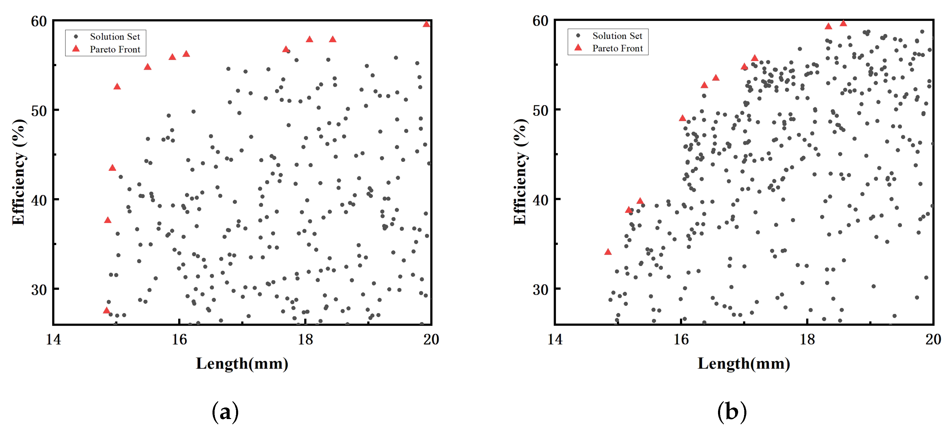
The parameter variation ranges are constrained by baseline design values to ensure physical feasibility. Multi-objective optimization is performed in KlyH using the NSGA-II and OMOPSO algorithms with the following settings: population size of 1000, maximum number of iterations set to 10, mutation probability of 0.07, and crossover probability of 0.9. The resulting Pareto fronts for each algorithm are shown in Figure 8, demonstrating trade-offs between compactness and efficiency.

4.3. Post-Processing of Optimization Results

Upon completion of the optimization process, a set of engineering-compliant solutions is selected from the two Pareto-optimal sets, balancing performance objectives with practical feasibility. The corresponding cavity parameters are summarized in

Table 2. Optimized parameters of each cavity.

Cavity ID	$(\mathit{R}/\mathit{Q})/\mathbf{\Omega }$	M	${\mathit{Q}}_{\mathit{ext}}$	${\mathit{Q}}_0$	$\mathit{f}/$MHz	$\mathit{Z}/$cm	$\mathit{d}/$mm
Input cavity	172.1	0.71	192	2235	10,000.9	0	5.0
Buncher cavity I	171.8	0.71	95,000	4870	10,004.6	4.18	5.0
Buncher cavity II	195.5	0.33	95,000	4199	19,835.8	5.61	1.8
Buncher cavity III	158.0	0.72	95,000	4580	10,103.3	7.90	4.5
Buncher cavity IV	188.6	0.33	95,000	4372	19,802.7	10.61	2.2
Buncher cavity V	169.8	0.70	95,000	4783	10,363.3	14.37	4.8
Output cavity	185.5	0.70	28	5138	9903	17	5.5

.

Using the predefined computational parameters, the 1D simulation validations in KlyH and AJDISK yield the following results:

• KlyH: $P_{out}$ = 749.12 MW, $\eta$ = 55%, $Gain$ = 53 dB;
• AJDISK: $P_{out}$ = 786.24 MW, $\eta$ = 53%, $Gain$ = 57 dB.

In KlyH, the cavity parameters—gap impedance ($Z_{L,n}$), loaded quality factor ($Q_{L,n}$), gap voltage magnitude ($V_{gap,n}$), and gap voltage phase (${\phi }_{gap,n}$)—are tabulated in

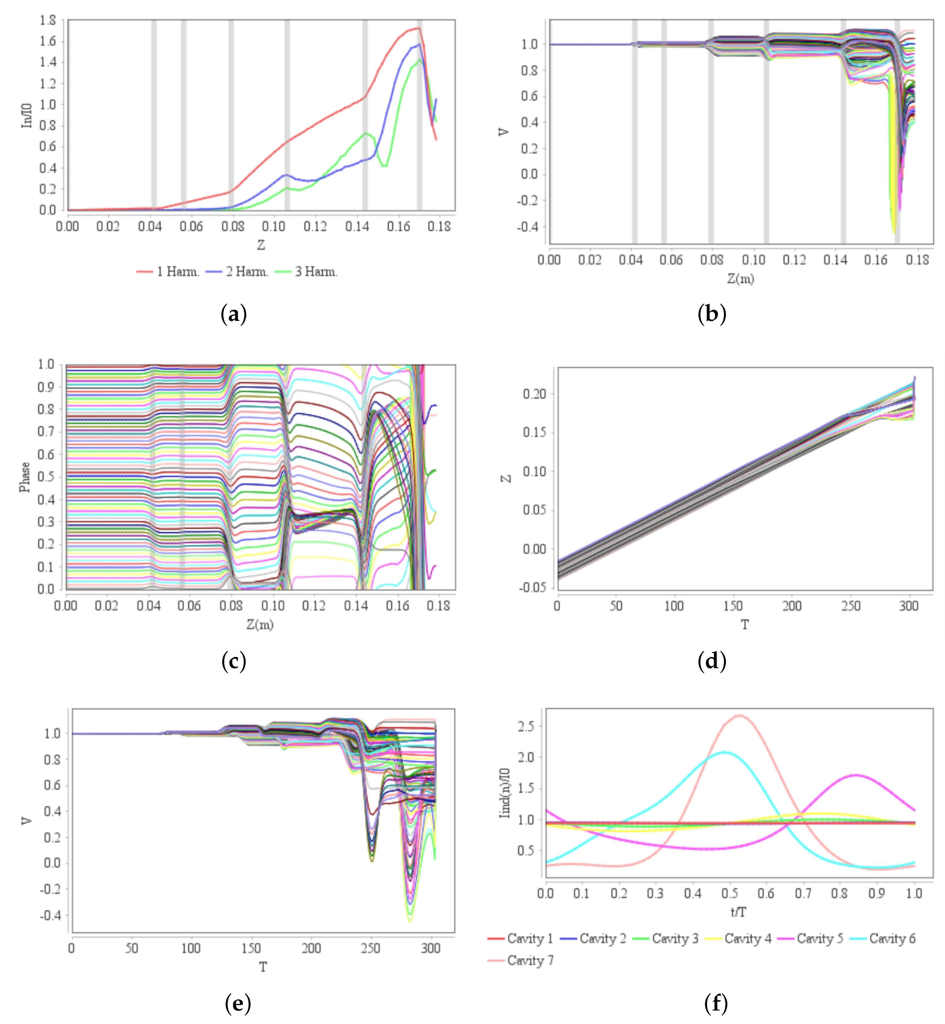
Table 3. Output Parameters of Each Cavity Generated by KlyH.

Cavity ID	${\mathit{Z}}_{\mathit{L}}/\mathbf{\Omega }$	${\mathit{Q}}_{\mathit{L}}$	${\mathit{V}}_{\mathit{gap}}/$kV	${\mathit{\phi }}_{\mathit{gap}}/$rad
Input cavity	18	103	4109	0.0
Buncher cavity I	38	224	41,280	0.2
Buncher cavity II	11	221	4186	2.3
Buncher cavity III	8	253	121,793	3.0
Buncher cavity IV	9	214	190,077	0.7
Buncher cavity V	2	230	228,816	−1.2
Output cavity	4	25	494,648	2.5

.

Figure 9 illustrates the key physical distributions.

5. Three-Dimensional PIC Simulation Validation with Optimized Parameters

To validate the accuracy of KlyH’s optimization results, 3D PIC simulations were conducted using the optimized structural parameters. These simulations comprehensively model beam–field interactions and evaluate klystron performance under realistic operating conditions. A comparative analysis with the 1D results from both KlyH and AJDISK was conducted to validate the effectiveness of the proposed 1D optimization design.

5.1. Three-Dimensional PIC Simulation

The 3D klystron model was re-adjusted with optimized drift tube lengths and buncher cavity frequencies. CST Particle Studio was employed for the simulations, extracting key metrics including efficiency, output power, gain, and cavity gap voltage distributions. To ensure computational accuracy and solution convergence, refined meshing and adaptive time-stepping strategies were implemented. The critical CST simulation parameters are listed in

Table 4. Beam parameters.

Parameter Name	Value
$U_{\mathrm{beam}}$/kV	375
$I_{\mathrm{beam}}$/kA (total)	3.380
$I_{\mathrm{beam}}$/A (single)	115
$R_{\mathrm{beam}}$/$\Omega$	102
$N_{\mathrm{beam}}$	32
$r_{\mathrm{center}}$/mm	45
$r_{\mathrm{tube}}$/mm	3.6
$r_{\mathrm{beam}}$/mm	2.24
${\mu }_k/{\mu }_{\mathrm{perv}}$ (single beam)	0.5008
${\mu }_k/{\mu }_{\mathrm{perv}}$ (total)	16.0256
Brillouin/G	1487.08
$N_{\mathrm{cavity}}$	7

.

Figure 10a shows the output microwave power versus time, yielding 726 MW of output power with 53% efficiency. Figure 10b displays the axial electron velocity distribution, confirming no electron reflux phenomenon.

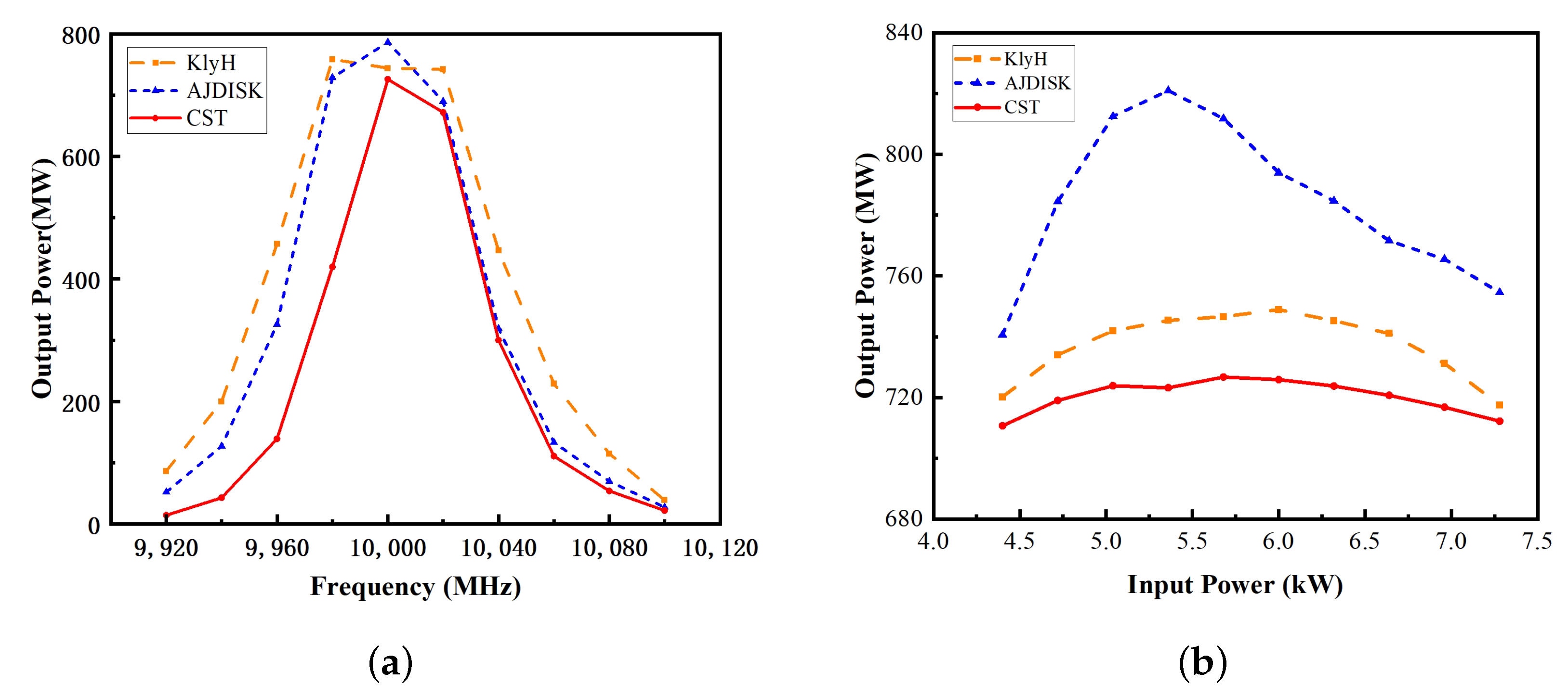
Figure 11a presents a comparison of output power versus frequency among the KlyH, AJDISK, and CST simulations. All three methods exhibit consistent overall trends, showing pronounced power peaks near the central frequency and rapid power decline with frequency deviation, which validates the strong predictive capability of the 1D simulation for 3D results. In terms of numerical accuracy, KlyH and AJDISK yield closely aligned computational results, while both demonstrate acceptable deviations from the 3D CST simulations, meeting engineering application requirements.

Figure 11b compares output power versus input power characteristics simulated using KlyH, AJDISK, and CST. All three tools show consistent output power trends, with the KlyH results exhibiting close agreement with the CST data (both deviations fall within an acceptable range.). KlyH achieves 2.7× faster computation than AJDISK in large-signal simulations (3 s/run vs. 8 s/run), effectively accelerating klystron optimization iterations.

5.2. Comparative Analysis of Key Parameters

Table 5. Comparative analysis of simulation results.

Software	Cavity ${\mathit{V}}_{\mathit{gap},\mathit{n}}$/kV							${\mathit{P}}_{\mathit{out}}/$MW	$\mathit{Gain}/$dB	$\mathit{\eta }/\%$
	Input	I	II	III	IV	V	Output
KlyH	4.1	41.3	4.2	121.8	190.1	228.8	494.6	749.1	53	55
AJDISK	4.1	59.9	6.1	150.9	204.3	243.3	512.4	786.2	53	57
CST	4.1	51.4	7.2	130.5	181.1	211.7	472.1	726.4	51	53

presents a comparison between the 3D simulation results and the results calculated by the 1D software KlyH and AJDISK.

The comparative analysis of cavity gap voltages reveals the following trends:

• Buncher cavity 1: The AJDISK results exceed the 3D simulation values, while the KlyH predictions are lower.
• Buncher cavity 2: Both AJDISK and KlyH yield lower values than the 3D simulations.
• Buncher cavities 3–5: The AJDISK and KlyH results are higher than the 3D simulations.
• Output cavity: Both tools overestimate compared to the 3D results.

The overall performance metrics (efficiency, gain, electronic efficiency) show strong consistency across all three tools.

6. Conclusions

This paper presents a detailed introduction to the development and application of KlyH, a new large-signal simulation software for klystrons. Through the optimization design of an X-band seven-cavity klystron, the application of KlyH in 1D simulation and optimization is demonstrated. This process involves acquiring initial parameters from a 3D structure, defining optimization objectives and variables, applying multi-objective optimization algorithms to obtain Pareto-optimal solutions, and validating the results via 1D simulations using KlyH. Based on optimized parameters, a reconstructed 3D model is subjected to 3D simulation, with its results compared against 1D simulations from both KlyH and AJDISK. Key analyses focus on the gap voltage distributions across cavities and overall performance metrics. The results indicate that KlyH can accurately predict critical performance parameters of klystrons, with the optimized klystron exhibiting high efficiency and output power in 3D simulations. However, KlyH currently has several limitations that need to be addressed in future work. It lacks a self-consistent space-charge field computation, which may reduce accuracy under strong space-charge conditions. The high-frequency cavity parameters such as $R/Q$ and Q are assumed constant during optimization, potentially limiting accuracy when cavity geometry changes significantly. The beam dynamics model is based on the disk-beam approximation and does not account for transverse or edge effects, which can be significant for large-radius or multi-beam structures. Furthermore, although KlyH has been validated against 3D PIC simulations for a typical seven-cavity RKA, its applicability to unconventional designs such as multi-gap cavities requires further investigation. Future improvements will focus on enhancing space-charge modeling, enabling geometry-dependent cavity parameter updates, and incorporating more detailed beam dynamics. The applicability of KlyH to non-standard structures will be extended and systematically validated. Moreover, integrating artificial intelligence algorithms, including deep learning and reinforcement learning, is planned to improve optimization efficiency, accelerate convergence, and enhance the robustness of the design process. Additionally, the software will be calibrated with experimental data to strengthen its practical utility, thereby establishing a robust theoretical and practical foundation for high-performance klystron optimization.

References

- Xiao, R.Z.; Deng, Y.Q.; Wang, Y.; Song, Z.; Li, J.; Sun, J.; Chen, C. Power combiner with high power capacity and high combination efficiency for two phase-locked relativistic backward wave oscillators. Appl. Phys. Lett. 2015, 107, 133502. [Google Scholar] [CrossRef]
- Varian, K.R. Power combining in a single multiple-diode cavity. In Proceedings of the 1978 IEEE-MTT-S International Microwave Symposium Digest, Ottawa, ON, Canada, 27–29 June 1978; pp. 344–345. [Google Scholar]
- Friedman, M.; Krall, J.; Lau, Y.Y.; Serlin, V. Externally modulated intense relativistic electron beams. J. Appl. Phys. 1988, 64, 3353–3379. [Google Scholar] [CrossRef]
- Friedman, M.; Serlin, V.; Lampe, M.; Hubbard, R. Applications of relativistic klystron amplifier technology. In Proceedings of the AGARD Conference Proceedings, Seville, Spain, 2–5 October 1995. [Google Scholar]
- Friedman, M.; Krall, J.; Lau, Y.Y.; Serlin, V. Relativistic Klystron Amplifier. In Proceedings of the Microwave and Particle Beam Sources and Propagation, Los Angeles, CA, USA, 13–15 January 1988; SPIE: Cergy-Pontoise, France, 1988; Volume 873, pp. 2–9. [Google Scholar]
- Wu, Y.; Li, Z.H.; Xu, Z.; Ma, Q.S.; Xie, H.Q. An S-band high gain relativistic klystron amplifier with high phase stability. Phys. Plasmas 2014, 21, 113107. [Google Scholar] [CrossRef]
- Sun, L.; Huang, H.; Li, S.; Liu, Z.; He, H.; Xiang, Q.; He, K.; Fang, X. Investigation on high-efficiency beam-wave interaction for coaxial multi-beam relativistic klystron amplifier. Electronics 2022, 11, 281. [Google Scholar] [CrossRef]
- Bao, B.Y. Research on Ku-Band Overmoded Relativistic Klystron Amplifier. Ph.D. Thesis, National University of Defense Technology, Changsha, China, 2017. [Google Scholar] [CrossRef]
- Liu, Z.; Song, F.; Jin, H.; Jin, X.; Huang, H.; Li, S. Coherent Combination of Power in Space with Two X-Band Gigawatt Coaxial Multi-Beam Relativistic Klystron Amplifiers. IEEE Electron Device Lett. 2022, 43, 284–287. [Google Scholar] [CrossRef]
- Xiang, Y.; Jin, Z.; Zhang, D.; Zhang, J.; Yang, K.; Zhou, F. A C-band relativistic backward wave oscillator optimized by multiobjective algorithms. IEEE Trans. Electron Devices 2025, 72, 2561–2567. [Google Scholar] [CrossRef]
- Haynes, W.B.; Fazio, M.V.; Carlsten, B.E.; Stringfield, R.M. Experimental and theoretical development towards a 500 MW, one-microsecond, L-band relativistic klystron amplifier. AIP Conf. Proc. 1995, 337, 2042–2049. [Google Scholar] [CrossRef]
- Behtouei, M.; Spataro, B.; Di Paolo, F.; Leggieri, A. The Ka-Band High Power Klystron Amplifier Design Program of INFN. arXiv 2020, arXiv:2011.12809. [Google Scholar] [CrossRef]
- Ju, J.; Zhang, J.; Qi, Z.; Yang, J.; Shu, T.; Zhang, J.; Zhong, H. Towards coherent combining of X-band high power microwaves: Phase-locked long pulse radiations by a relativistic triaxial klystron amplifier. Sci. Rep. 2016, 6, 30657. [Google Scholar] [CrossRef]
- Yang, W.; Xie, H.; Zhou, X. Mode control in a high gain relativistic klystron amplifier with 3 GW output power. Chin. Phys. C 2014, 38, 017001. [Google Scholar] [CrossRef]
- Fazio, M.; Carlsten, B.; Faehl, R.; Kwan, T.; Rickel, D.; Stringfield, R.; Tallerico, P. High-Current Relativistic Klystron Amplifier Development for Microsecond Pulse Lengths; Los Alamos National Laboratory Report; Los Alamos National Laboratory: Los Alamos, NM, USA, 1995. [Google Scholar]
- Fuks, M.; Schamiloglu, E.; Benford, J. Operation of a multigigawatt relativistic klystron amplifier. Proc. SPIE 1989, 1061, 34–41. [Google Scholar] [CrossRef]
- Behtouei, M.; Spataro, B.; Faillace, L.; Carillo, M.; Leggieri, A.; Palumbo, L.; Migliorati, M. Relativistic approach to a low perveance high quality matched beam for a high efficiency Ka-Band klystron. arXiv 2021, arXiv:2109.03520. [Google Scholar]
- Behtouei, M.; Spataro, B.; Di Paolo, F.; Leggieri, A. Simulations for a low-perveance high-quality beam matching of a high efficiency Ka-band klystron. arXiv 2020, arXiv:2012.03737. [Google Scholar]
- Meng, C.; Xiao, O.Z.; Pei, S.L.; Wang, S.C.; Zhou, Z.S.; He, X. Optimization of Klystron Efficiency with MOGA. In Proceedings of the IPAC, Vancouver, BC, Canada, 4 April 2018; pp. 2936–2939. [Google Scholar] [CrossRef]
- Sun, L.; Huang, H.; Li, S.; Liu, Z.; Tan, J.; Wang, P.; Basu, B.N.; He, H.; He, K.; Duan, Z. Short-Length, High-Efficiency S-Band Coaxial Cavity Relativistic Multibeam Klystron Amplifier for Potential High Power Microwave Application. IEEE Electron Device Lett. 2022, 43, 1760–1763. [Google Scholar] [CrossRef]
- Xie, B.; Zhang, R.; Tian, L.; Li, H.; Wang, Y.; Liu, K. Auto-machine learning-based W-band high-efficiency oscillator design. IEEE Trans. Electron Devices 2024, 71, 6350–6356. [Google Scholar] [CrossRef]
- Xia, G.; Liu, X.; He, Y.; Zhong, J.; Jin, Z.; Zhu, F.; Zhang, Z.; Liu, W. GA-BP neural networks for optimal design of multistage depressed collector for 340-GHz traveling wave tubes. IEEE Trans. Electron Devices 2024, 71, 7066–7073. [Google Scholar] [CrossRef]
- Tien, P.K.; Walker, L.R.; Wolontis, V.M. A large signal theory of traveling-wave amplifiers. Proc. IRE 1955, 43, 260–277. [Google Scholar] [CrossRef]
- Ding, Y. Theory and Computational Simulation of High-Power Klystrons; National Defense Industry Press: Beijing, China, 2008. [Google Scholar]
- Lingwood, C.; Kowalcyzk, R.; Constable, D.; Burt, G. Developing Sheet Beam Klystron Simulation Capability in AJDISK. IEEE Trans. Electron Devices 2017, 64, 1701–1707. [Google Scholar] [CrossRef]
- Cai, J.; Syratchev, I. KlyC: 1.5-D Large-Signal Simulation Code for Klystrons. IEEE Trans. Plasma Sci. 2019, 47, 1734–1741. [Google Scholar] [CrossRef]
- Yonezawa, H.; Okazaki, Y. One-Dimensional Disk Model Simulation for Klystron Design. Technical Report SLAC-TN-84-5, Stanford Linear Accelerator Center. 1984. Available online: https://www.osti.gov/biblio/6751246 (accessed on 23 May 2025).
- Sakanaka, S.; Kamitani, T.; Oguri, Y.; Saito, S.; Furukawa, K.; Hasegawa, K.; Yoshida, M.; Oide, K.; Funahashi, Y.; Kuriki, M.; et al. Development of DISKLY for High-Power Klystron Design. In Proceedings of the 8th Linear Accelerator Conference (LINAC), Geneva, Switzerland, 26–30 August 1996; pp. 465–467. [Google Scholar]
- Seshadri, A. A fast elitist multiobjective genetic algorithm: NSGA-II. MATLAB Cent. 2006, 182, 182–197. [Google Scholar]
- Jiang, H. Study on Multi-Objective Optimization Particle Swarm Algorithm. Ph.D. Thesis, Xiangtan University, Xiangtan, China, 2006. [Google Scholar]
- Zitzler, E.; Laumanns, M.; Thiele, L. SPEA2: Improving the Strength Pareto Evolutionary Algorithm; TIK-Report 103; Computer Engineering and Networks Laboratory (TIK), ETH Zurich: Zurich, Switzerland, 2001. [Google Scholar]
- Zhang, Q.; Li, H. MOEA/D: A multiobjective evolutionary algorithm based on decomposition. IEEE Trans. Evol. Comput. 2007, 11, 712–731. [Google Scholar] [CrossRef]