Design of a Comprehensive Intelligent Traffic Network Model for Baltimore with Consideration of Multiple Factors

Abstract

The collapse of Baltimore’s Francis Scott Key Bridge in March 2024 has stressed the need for urban traffic network optimization within smart city initiatives. This paper utilizes the ARIMA model to forecast what traffic would have been like if the bridge had not collapsed, giving us a benchmark to assess the impact. It then identifies the roads most affected by comparing these forecasts with the actual post-collapse traffic data. To address the increased demand for efficient public transport, we propose an intelligent bus network model. This model uses principal component analysis and grid segmentation to inform decisions on increasing bus stations and adjusting bus frequencies on key routes. It aims to satisfy stakeholders by enhancing service coverage and reliability. The research also presents a comprehensive traffic model that leverages principal component analysis, genetic algorithms, and KD-tree to evaluate overall and directional traffic flow, providing strategic insights into congestion mitigation. Furthermore, it examines traffic safety issues, including accident-prone areas and traffic signal intersections, to offer recommendations. Finally, the study evaluates the effectiveness, stability, and benefits of the proposed intelligent traffic network model, aiming to improve the city’s traffic infrastructure and safety.

1. Introduction

The transportation system is the lifeblood of a city, playing a crucial role in various essential functions, including daily commuting for residents, travel for visitors, and the passage of tourists. For a metropolis with a population of millions, the design of an efficient transportation system is undoubtedly a key factor in showcasing the city’s character and facilitating the convenience of its residents [1]. The tourism industry, transportation sector, and even local industries are all significantly influenced by how well the transportation system is designed. A factory located in an area with poor transportation access and frequent congestion is unlikely to operate at high efficiency [2]. Unfortunately, many aging cities are grappling with increasingly severe traffic problems due to outdated infrastructure and planning [3]. Meanwhile, with the continuous development of technology, many traditional cities are gradually transforming towards smart cities, which has also led to more regulation and research on intelligent transportation networks [4,5].

Baltimore boasts a busy port and a strong shipping industry, but this has been severely impacted by the collapse of the Francis Scott Key Bridge, which connects the port, caused by a cargo ship collision in March 2024 [6,7]. As a key port of the United States, the failure of Baltimore port has caused great loss to the global shipping market, as well as the traffic situation of Baltimore city. The daily commuting of residents working in shipping has been disrupted, goods waiting to be transported and exported to the port are delayed or forced to take longer routes, and traffic congestion in the city center has worsened. Thanks to a newly implemented infrastructure development plan, the Baltimore government aimed to address these issues and take the opportunity to improve the past unwise planning that had divided communities with highways. In light of this, it is essential to build a model that describes the current state of Baltimore’s transportation system in order to explore the impacts caused by these problems and find the best solutions to resolve them. At the same time, in view of this phenomenon, the design of a smart city network model for different stakeholders is also crucial for the future urban development.

2. Related Work

In terms of the construction of smart cities, Albino et al. [8] provided a detailed explanation and introduction of the definition, dimensions, and corresponding measures of smart cities in 2015. Hollands et al. [9] and Chourabi et al. [10] also analyzed and looked forward to the possible future development and framework of smart cities. An intelligent transportation network is an indispensable part of realizing smart cities.

Smart transportation networks are integral to the development of smart cities, aiming to enhance urban mobility, safety, and efficiency through advanced technologies. These networks leverage sensors, data analytics, and AI to collect and analyze vehicle movement and traffic patterns, optimizing transport systems to reduce emissions, improve safety, alleviate traffic congestion, and boost quality of life [11]. The integration of intelligent transportation systems (ITS) with traditional transportation frameworks is crucial for achieving sustainable urban mobility [11,12].

The construction of smart transportation networks is closely linked to the broader development of smart cities. Smart transportation systems are foundational to smart cities, addressing critical issues like traffic congestion, safety, and environmental impact [13,14]. By optimizing transportation networks, smart cities can achieve higher efficiency in mobility, which is essential for the overall quality of urban life [13,14]. Moreover, smart transportation networks contribute to the sustainability goals of smart cities by reducing emissions and improving energy efficiency [13].

Traffic flow prediction is a critical component of ITS, enabling the forecasting of vehicular movement patterns based on historical and real-time data. Accurate traffic flow prediction helps in reducing congestion, optimizing road capacity, and improving travel planning [15,16,17,18]. Various machine learning and deep learning techniques, such as Long Short-Term Memory (LSTM), Convolutional Neural Networks (CNNs), and Vision Transformers (VTs), have been employed to enhance prediction accuracy [19,20,21,22]. These models consider spatial and temporal dependencies, weather conditions, and social events to provide reliable traffic forecasts [20,21,22].

As an important indicator for evaluating and optimizing transportation networks, Guo et al. [23] have designed a unified spatiotemporal and frequency attention method for traffic flow prediction. Zhou et al. [24] proposed a multi-variate partial gray prediction model based on second-order traffic flow kinematic equations. Li et al. [25] conducted a systematic evaluation of the generative adversarial network used for traffic state prediction. In the research of intelligent transportation networks, Parsa et al. [26] used XGBoost and SHAP for real-time accident detection and feature analysis, while Yang et al. [27] designed a micro traffic simulator for evaluating dynamic traffic management systems. Zhu et al. [28] proposed a multi-agent deep reinforcement learning method for large-scale traffic signal control, and research on multi-level and multi-dimensional intelligent transportation networks is constantly being valued and implemented.

This paper began with the collapse of the Francis Scott Key Bridge. Initially, the ARIMA algorithm was utilized to forecast the Average Annual Daily Traffic (AADT) and Average Annual Weekly Day Traffic (AAWDT) volumes had the bridge not collapsed, and these projections were compared with the actual post-collapse values to identify the roads most severely impacted by the event. Building on this foundation, we took Baltimore city as a case study and proposed two distinct urban traffic network optimization models for different travel demographics. We introduced an intelligent public transportation network model aimed at the daily life of urban residents, while also applying genetic algorithms and KD-tree designs to the existing traffic congestion and flow distribution in Baltimore to develop an intelligent road traffic network model. The paper conducted a detailed analysis on the stability of the current model and the accident safety of existing roads, and provided a perspective on the future development of intelligent transportation networks.

Considering the current state of research, we have identified the following issues that warrant attention. First, there is insufficient focus on the traffic changes in Baltimore following the collapse of the Francis Scott Key Bridge. Second, there is still a certain gap in the construction of interdisciplinary, multi-factor integrated models for public transportation and road traffic.

This paper begins with the collapse of the Francis Scott Key Bridge, utilizing the ARIMA algorithm to predict the Annual Average Daily Traffic (AADT) and Annual Average Weekday Traffic (AAWDT) under the assumption that the bridge had not collapsed. These predictions were then compared with the actual post-collapse data to identify the roads most affected by the event. Building on this analysis, we took Baltimore city as our case study and proposed two urban traffic network optimization models tailored to the different travel characteristics of city residents. Not only did we use PCA and grid segmentation to construct an intelligent public transportation network model for city residents’ daily lives, but we also innovatively integrated mature technologies such as statistical dimension reduction, topological redundancy measurement, spatial indexing, and genetic algorithms to build a brand-new, interdisciplinary intelligent road analysis model. Specifically, we used Principal Component Analysis (PCA) to automatically extract the weights of multiple traffic indicators, incorporated network redundancy into congestion assessment, and utilized KD-tree to quickly generate candidate connections, ultimately achieving optimal path selection through genetic algorithms. This end-to-end process design effectively compensates for the limitations of single methods in road network congestion mitigation applications. Moreover, our research focuses not only on the traffic pressure of individual road segments but, more importantly, on the overall robustness of the network, with “alternative path availability” as the core optimization goal. This approach breaks through traditional congestion-alleviation strategies that are mainly based on shortest paths or capacity enhancement. By reorganizing and adapting various classic algorithms to specific scenarios, we have proposed at the theoretical framework level an “integrated optimization oriented by network topological redundancy,” which is itself an innovative paradigm that can be generalized to other network systems (such as electricity, communication, etc.). This paper provides a detailed analysis of the stability of the current model and the accident safety of existing roads, conducts model validity analysis and simulation verification, and offers prospects for the future development of intelligent transportation networks.

3. Materials and Methods

3.1. Data Preprocessing

The data [29,30,31,32,33] provided by an official government website include the codes, start and end points and routes of the major and secondary roads in Baltimore city, and information about bridges and channels. It also contains the locations of intersections for various transportation modes (including general roads, highways, railways, and sidewalks), as well as the stations and passenger flow for major public transportation modes. Additionally, the dataset includes traffic flow data for each road segment from 2014 onward, including the annual average daily traffic (AADT), annual average weekday traffic (AAWDT), proportion of peak-hour traffic, and the distribution of traffic flow in different directions.

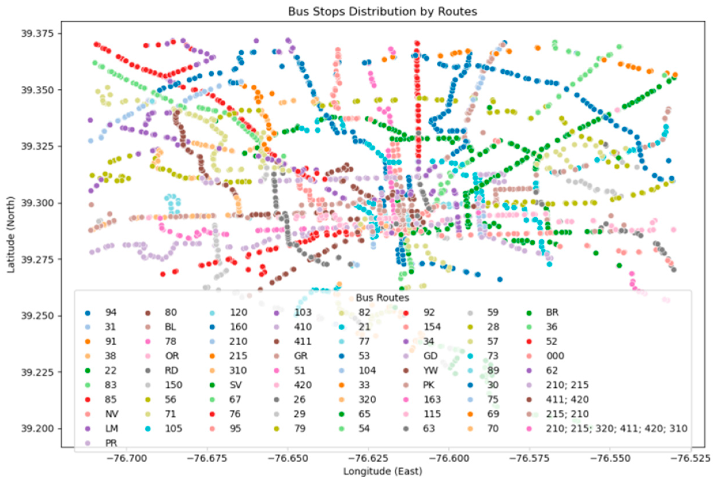
The data provided are large but not in order. To ensure the uniformity of the data, we made a series of procession. We used the search algorithm to replace the whole name of the roads with their abbreviation. We constructed maps of the bus routes and AADT to visually figure out the change of the traffic, as is shown in Figure 1.

We can observe from the figure that the southern part of Baltimore is the downtown, in which the bus routes and important roads concentrate, and we can see that the distribution of traffic is relatively uneven. The distribution of bus stations is denser in urban areas and sparser in suburban areas, with bus stations being particularly concentrated near the port.

3.2. The Impact of Emergencies on Urban Transport Networks: The Case of the Collapse of the Francis Scott Key Bridge

We handled this problem following the steps in Figure 2.

We found the relative position of Francis Scott Key Bridge in the chart (Figure 3).

The collapsed bridge is marked in the middle of the map. From the map we can discover that there are not many bridges to connect the two parts next to the bay. We can guess that due to the collapse of Francis Scott Key Bridge, other passages crossing the bay would have larger traffic flow.

We employed the ARIMA algorithm to finish the first step of Section 3.2. The ARIMA algorithm is a statistical method used for time series analysis and forecasting, consisting of three main components: Autoregression (AR), Integration (I), and Moving Average (MA). The autoregressive (AR) part represents the linear relationship between the current value and a number of past values [34]. The AR(p) model is represented as follows:

$$y_t=c+{\varphi }_1{y}_{t-1}+{\varphi }_2{y}_{t-2}+\cdots +{\varphi }_p{y}_{t-p}+{\epsilon }_t$$

(1)

where c is a constant, ${\varphi }_1, {\varphi }_2, \dots , {\varphi }_n$ are the regression coefficients, and ${\epsilon }_t$ is the random error term. In this case, we use the data from the first eight years to predict the current AADT and AAWDT in Baltimore city assuming that the bridge had not collapsed.

The integration(I) component is used to handle the non-stationarity of time series data, converting non-stationary series into stationary series. First-order differencing is represented as follows:

$$y_t^{\prime }=y_t-y_{t-1}$$

(2)

where $y_t^{\prime }$ is the first-order integrated series. Higher-order differencing can be achieved by repeatedly applying first-order integrating. For example, second-order integrating is represented as follows:

$$y_t^{″}=y_t^{\prime }-y_{t-1}^{\prime }=(y_t-y_{t-1})-(y_{t-1}-y_{t-2})=y_t-2y_{t-1}+y_{t-2}$$

(3)

where $y_t^{″}$ is the second-order integrated series. After multiple integrating steps, the traffic data will have a certain degree of stationarity.

Lastly, in the Moving Average (MA) model, the current value (the predicted AADT and AAWDT before the bridge collapse) is related to past q random error terms as follows:

$$y_t=\mu +{\epsilon }_t+{\theta }_1{\epsilon }_{t-1}+{\theta }_2{\epsilon }_{t-2}+\cdots +{\theta }_{\mathrm{q}}{\epsilon }_{t-q}$$

(4)

where $\mu$ is the mean, and ${\theta }_1$, ${\theta }_2$,…,${\theta }_{\mathrm{q}}$ are the moving average coefficients.

Combining these three models, the $ARIMA(p, d, q)$ model can be represented as follows:

$$\varphi \left(B\right)\left(1-B\right)d{y}_t=\theta \left(B\right){\epsilon }_t$$

(5)

where B is the backshift operator,

$$\varphi \left(B\right)=1-{\varphi }_1{B}_1-{\varphi }_2{B}_2-\cdots -{\varphi }_p{B}_p$$

(6)

$$\theta \left(B\right)=1+{\theta }_1{B}_1-{\theta }_2{B}_2-\cdots -{\theta }_q{B}_q$$

(7)

The values of p and q are initially determined by examining the ACF and PACF plots, and the optimal model parameters are selected using information criteria like AIC and BIC.

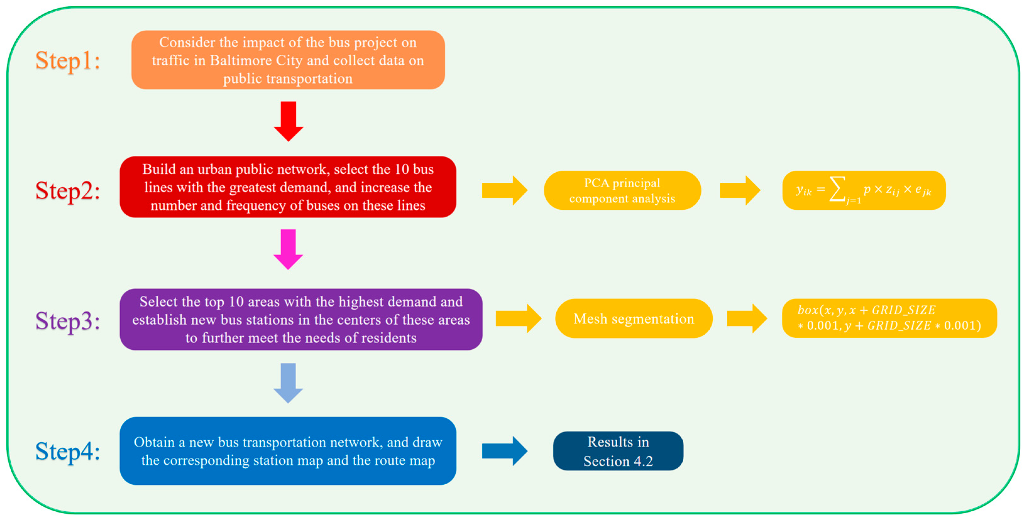
3.3. Scenario 1: Public Transport Improvement Strategies for Urban Residents: Optimization of the Network of Urban Public Transport Systems

We handled this problem following the steps in Figure 4.

3.3.1. Principal Component Analysis

Principal Component Analysis (PCA) is a statistical method used to transform a set of possibly correlated variables into a set of linearly uncorrelated variables, principal components. We chose to use PCA because the dataset contains multiple correlated indicators with differences in scales and ranges. PCA can reduce dimensionality, eliminate redundancy, equalize the importance of each indicator, enhance the interpretability and stability of the model, and optimize computational efficiency, thereby providing support for subsequent analyses.

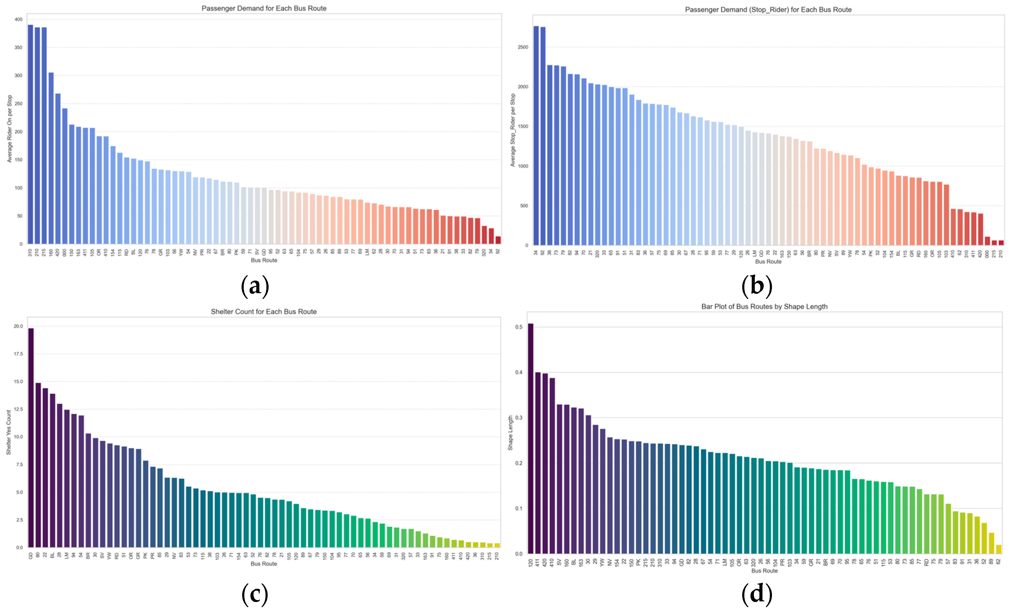
Before performing PCA, we calculated the mean values of the $Rider\_On$ and $Stop\_Rider$ (denoted as $Average\_Rider\_on$ and $Average\_Stop\_Rider$), the total number of stops for each route, the total count of stops with shelter, and the total length of each route recorded in the Shape_Length. Thus we selected four key indicators for the PCA: $Average\_Rider\_on$, $Average\_Stop\_Rider$, $Shelter\_Yes\_Count$, and Shape_Length. The situation of these four indicators is shown in Figure 5.

The specific formulas of the four indicators above are as follows:

• $Average\_Rider\_on:$

$$Average\_Rider\_on=\sum {\displaystyle \frac{{Rider\_on}_{i\mathrm{ }}}{m_i}}$$

(8)

${Rider\_on}_i$ represents the number of riders boarding at stop i, and $m_i$ represents the number of bus lanes stopping at this stop.

b.

$Average\_Stop\_Rider$:

$$Average\_Stop\_Rider=\sum {\displaystyle \frac{{Stop\_Rider}_j}{n_j}}$$

(9)

${Stop\_Rider}_j$ represents the number of riders at stop i, and $n_j$ represents the number of bus lanes stopping at this stop.

c.

$Shelter\_Yes\_Count$:

$$Shelter\_Yes\_Count=\sum p_k$$

(10)

$p_k$ takes the value of 1 if there is a shelter at this stop, otherwise it takes the value of 0.

We first standardize the original data to eliminate the effects of different units and the range differences between variables. The standardization formula is as follows:

$$z_{ij}={\sigma }_j{x}_{ij}-{\mu }_j$$

(11)

where $x_{ij}$ is the value of the j-th variable for the i-th sample, ${\mu }_j$ is the mean of the j-th variable, and ${\sigma }_j$ is the standard deviation of the j-th variable.

Next, we select the principal components from the aforementioned indicators. We begin by performing eigenvalue decomposition on the covariance matrix C to obtain the eigenvalues ${\lambda }_1,{\lambda }_2,\cdots ,{\lambda }_p$ and their corresponding eigenvectors e₁,e₂,…,e_p. The eigenvalue–eigenvector relationship is given by the following:

$$C{e}_k={\lambda }_k{e}_k$$

(12)

where $C$ is the covariance matrix, $e_k$ is the k-th eigenvector, ${\lambda }_k$ is the k-th eigenvalue, and p is the number of variables. The eigenvalues are arranged in descending order, and the corresponding eigenvectors are ordered accordingly. The magnitude of the eigenvalues indicates the amount of variance explained by the corresponding principal component. We select the top m largest eigenvalues and their corresponding eigenvectors as the principal components, as these m components explain most of the variance in the data.

Using the selected eigenvectors, we compute the coordinates of each sample in the principal component space, known as the principal component scores. The score of the i-th sample on the k-th principal component is given by the following:

$$y_{ik}={\sum }_{j=1}p\times z_{ij}\times e_{jk}$$

(13)

where $z_{ij}$ is the standardized value of the j-th variable for the i-th sample, and $e_{jk}$ is the j-th element of the k-th eigenvector. Based on the principal component scores, the components can be interpreted, and the weights can be adjusted accordingly. In this model, we adjust the weight of $Average\_Stop\_Rider$ and $Shelter\_Yes\_Count$, so that lower values of these indicators are preferred.

Table 1. Indicators with weights.

Indicator	Weights
$Average\_Rider\_On$	0.5086
$Average\_Stop\_Rider$	0.2823
$Shelter\_Yes\_Count$	0.1667
$Shape\_Length$	0.0424

shows the accurate weights of each indicator.

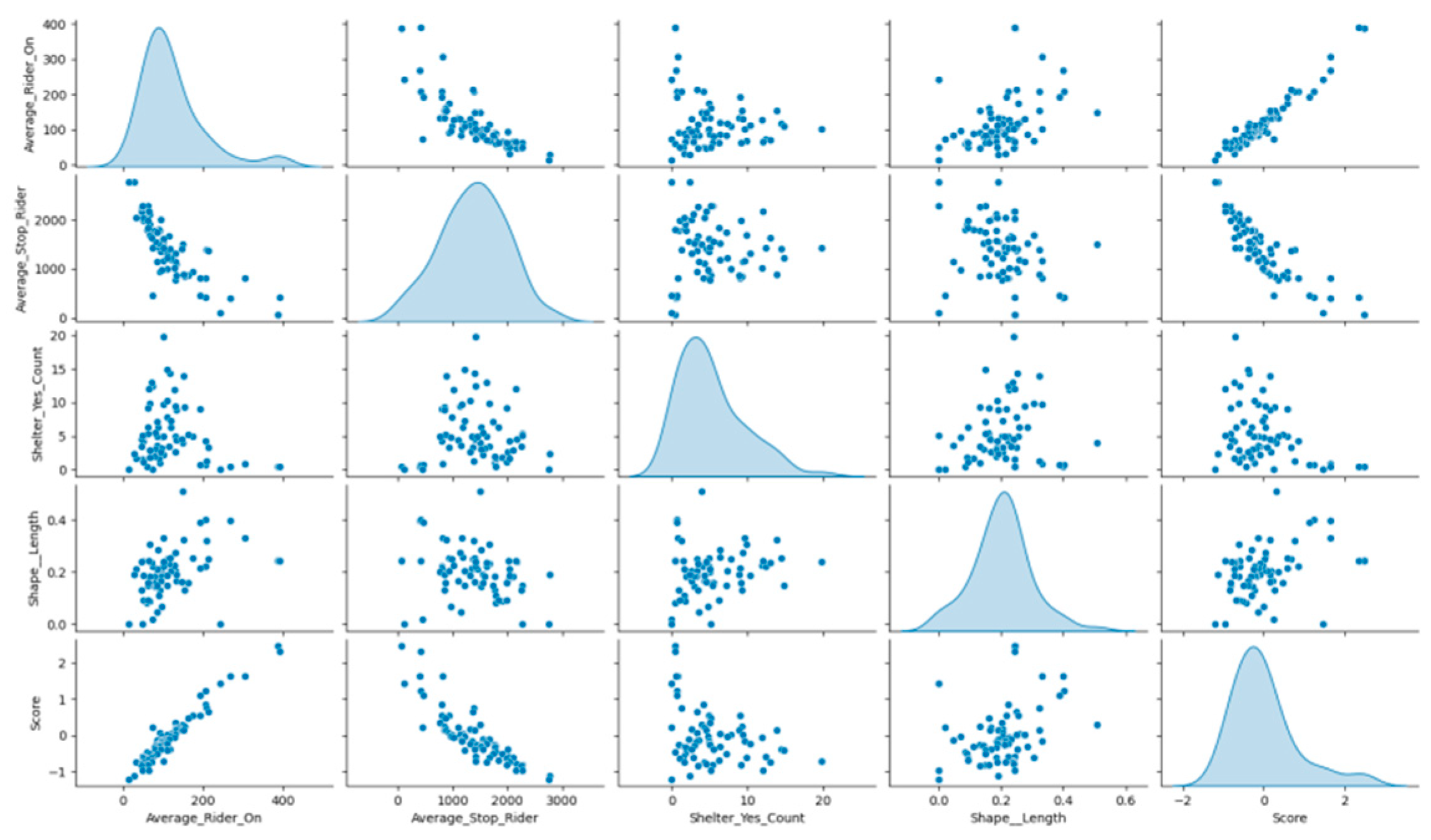
Finally, we calculated the composite score for each route and rank them. The top 10 routes with the highest composite scores are identified, indicating the routes that require an increase in bus numbers and frequency. The result is shown in Figure 6.

Figure 6 uses a scatter plot matrix to display the relationships between four key indicators used for optimizing the urban public transportation system and the composite score. The diagonal of the plot shows the distribution of each indicator individually, where both $Average\_Rider\_On$ and $Average\_Stop\_Rider$ exhibit an approximately normal distribution, whereas $Shelter\_Yes\_Count$ shows a skewed distribution, with most stops having a smaller number of shelters. The plots off the diagonal illustrate the relationships between two variables; for instance, there is a clear positive correlation between $Average\_Rider\_On$ and $Average\_Stop\_Rider$, indicating that stops with a higher number of riders boarding also tend to have more riders alighting. The relationship between $Shelter\_Yes\_Count$ and other variables is not apparent, suggesting that the number of shelters may have a minimal impact on the number of riders boarding and alighting. Additionally, the relationship between $Shape\_Length$ and both $Average\_Rider\_On$ and $Average\_Stop\_Rider$ is more complex and may involve non-linear associations. In the plots in the last column and row, the relationships between the composite score and each indicator are revealed, with the score showing a positive correlation with $Average\_Rider\_On$ and $Average\_Stop\_Rider$, indicating that routes with higher numbers of riders boarding and alighting have higher scores and might require increased bus service frequency. The relationship between $Shelter\_Yes\_Count$ and the score is not evident, which could imply that the number of shelters has little influence on the route score.

3.3.2. Grid Partition

To further alleviate the operational pressure on buses, we considered establishing new bus stations at certain points. We used the grid partitioning method to develop a standard evaluation system, scoring each grid cell. The higher the score is, the greater the demand for a bus station in that grid cell is. Finally, we will select grid cells with the top 10 highest scores to establish new bus stations at their center points.

The grid partitioning method involves dividing the urban area into equally sized grid cells, allowing for independent analysis and evaluation of each cell to determine the optimal locations for new bus stops. The advantage of this method is that it provides a systematic and standardized way to assess urban transportation needs, especially for the optimization of public transit services. By altering the size of the grids, the level of analysis detail can be adjusted to more accurately identify areas with high demand, thereby determining the number and locations of new bus stops. Smaller grids can offer more detailed analysis but may increase computational complexity, while larger grids might simplify the analysis process but could sacrifice some details. Therefore, selecting the appropriate grid size is crucial for ensuring the accuracy and practicality of the analysis results.

First, set some parameters, including grid size, the weight of the number of nodes, and the latitude and longitude range for predicting bus stations. We only used roads with the highway type “residential” from all edge data and checked whether such roads exist. If they do, we proceed with the processing.

Next, the model created a grid covering the specified latitude and longitude range. First, we defined the bounding box and obtained the projection range of the bounding box to generate grid cells. The generation formula is as follows:

$$box(x,y,x+GRID\_SIZE\ast 0.001,y+GRID\_SIZE\ast 0.001)$$

(14)

In this formular, x and y are the coordinates of the bottom-left corner of the grid cell, and $GRID\_SIZE$ is the grid size in meters. By iterating through the coordinates within the latitude and longitude range, we generate each grid cell and store it in the model.

Next, we calculate the number of residential roads within each grid cell. We perform a spatial join between the residential road data and the grid data and then group by grid cell to calculate the number of residential roads within each grid cell. Similarly, we calculate the number of bus stations and the number of nodes within each grid cell.

Finally, we calculate the comprehensive score for each grid cell with the following formula:

$$X=road\_count-bus\_stop\_count+node\_count\ast NODE\_WEIGHT$$

(15)

In this case, $X$ is the comprehensive score, $road\_count$ is the number of residential area roads, $bus\_stop\_count$ is the number of bus stations, $node\_count$ is the number of nodes, and $NODE\_WEIGHT$ is the weight of the node count.

We select the top 10 grid cells with the highest comprehensive scores and obtain the center points of these grid cells as the proposed locations for the bus stations.

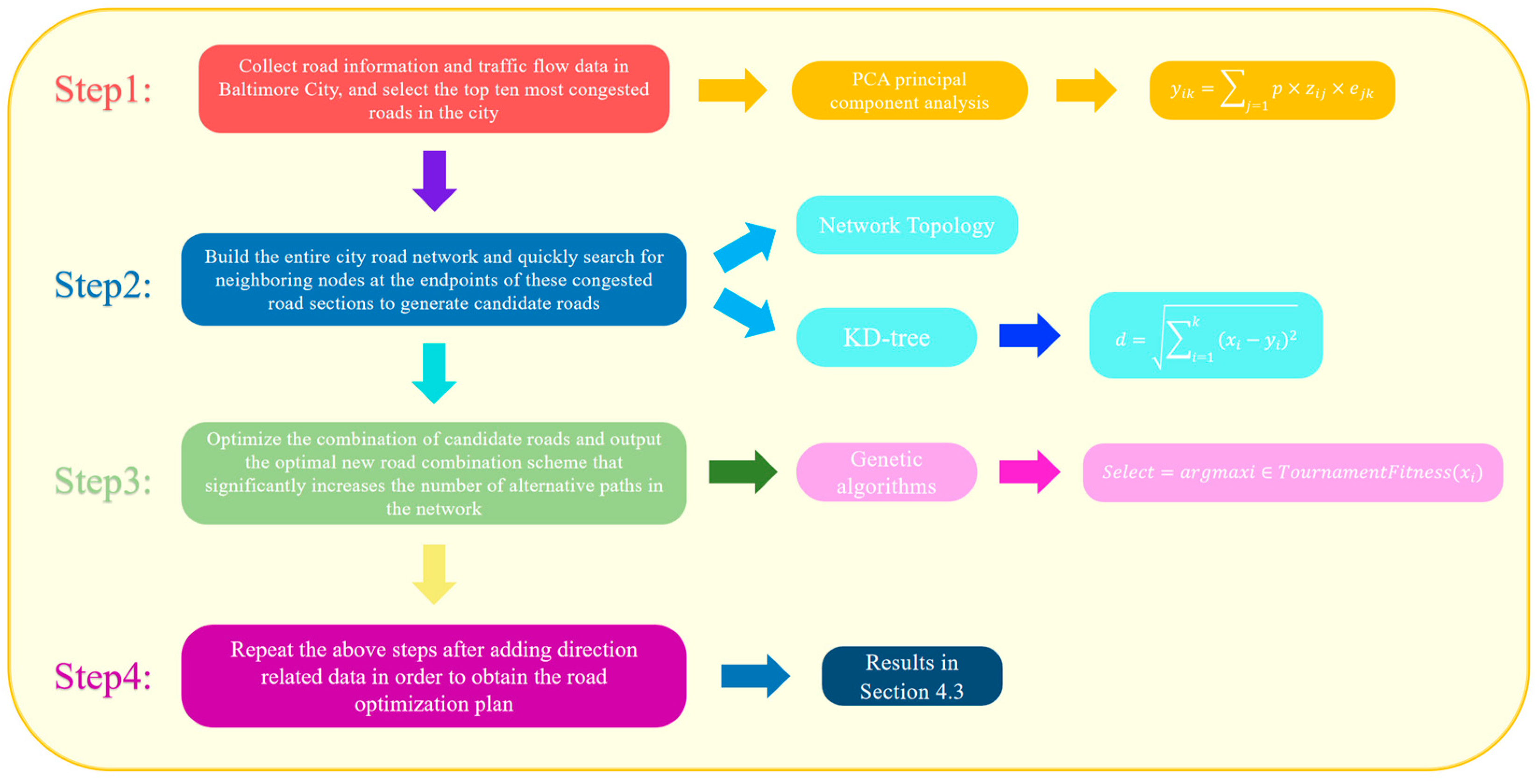
3.4. Scenario 2: Road Traffic Improvement Strategies for Urban Residents: Optimization Network of Urban Road Traffic Systems

In this section, taking Baltimore city as the subject of study, we innovatively integrated mature technologies such as statistical dimension reduction, topological redundancy measurement, spatial indexing, and genetic algorithms to construct a brand-new, interdisciplinary intelligent road analysis model. Specifically, we used Principal Component Analysis (PCA) to automatically extract the weights of various traffic indicators, incorporated network redundancy into the congestion assessment, and utilized KD-tree to quickly generate candidate connections, ultimately achieving optimal path selection through genetic algorithms. This end-to-end process design effectively compensates for the limitations of individual methods in the application of road network congestion mitigation. Moreover, our research not only focuses on the traffic pressure of individual road segments but, more importantly, starts from the overall robustness of the network, taking “alternative path availability” as the core optimization goal. This approach breaks through the traditional congestion-alleviation strategies that are mainly based on shortest paths or capacity enhancement, proposing an “integrated optimization oriented by network topological redundancy” strategy.

We handled this problem following the steps in Figure 7.

3.4.1. Principal Component Analysis

Before constructing the model of Section 3.4, let us first explain the process of obtaining road information.

• We first obtained basic information of the roads. First, we extracted data including the names of various roads in Baltimore city, along with the areas they pass through and the number of lanes. This information provided the foundational framework for our subsequent geographic location identification.
• Then we obtained basic information of important road nodes along with their osmid (OpenStreetMap ID). Using the osmid of these nodes, we could clearly identify the starting and ending points of each road, as well as the key intermediate nodes it passes through.
• Next, we obtained the longitude and latitude information of each node. By associating these coordinate details with the node osmid, we could accurately locate each node on the map.
• Finally, we integrated the information of all the roads from the above steps. Using osmid of each node and road, we extracted the geographic coordinates and sequentially connected these nodes. In this way, we could clearly depict the exact geographic locations of each road, providing accurate geographic data support for subsequent road analysis and applications.

Before performing principal component analysis, we first compiled data including the D-Factor, K-Factor, Number of Lanes, as well as the Annual Average Daily Traffic (AADT) from the past nine years (2014–2022), Annual Average Weekday Traffic (AAWDT), and AADT based on vehicle categories (for the current year only). These data were then standardized and transformed into six indicators: AADT, AAWDT, D-Factor, K-Factor, AVMT, and Number of Lanes.

Following a similar approach as in Section 3.3, we adjusted the weights of each indicator to further optimize the model. The specific weight distribution is shown in

Table 2. Indicators with weights.

Indicator	Weights
AADT	0.2235
AAWDT	0.2237
D-Factor	0.0690
K-Factor	0.1118
AVMT	0.1800
Number of Lanes	0.1920

.

Finally, we calculated the congestion score for each road as the weighted sum of the standardized indicators, and then sorted the data based on the congestion scores to identify the top 10 most congested roads.

3.4.2. Network Topology and KD-Tree Model

After constructing congestion scores based on statistical indicators, we used these scores to identify the top 10 critical road segments that are highly prone to congestion. Based on the endpoints of these segments, we constructed a graph that represents the structure of the entire urban road network.

We initially built a complete traffic network graph using network topology methods, where each node represents an intersection, and each edge represents a specific road segment. Through this topological structure, we can intuitively analyze the connectivity and structural characteristics of the entire road system. Especially during the construction process, by utilizing existing node and edge information, we can calculate the number of alternative paths for each critical segment, thereby reflecting the actual level of redundancy and robustness within the network.

To enhance the overall robustness of the network, our research no longer focuses solely on the traffic issues of these critical segments themselves. Instead, we start from the perspective of network topology, emphasizing the “availability of alternative paths”, which is to examine whether there are multiple alternative paths within a certain limit to disperse traffic pressure.

To this end, during the candidate road generation phase, we used the KD-tree [35] algorithm to rapidly perform nearest neighbor searches on the spatial coordinates of the endpoints of the top 10 congested segments, yielding a set of candidate roads that could be considered for addition. This process fully leverages the advantages of KD-tree in efficient nearest neighbor searches, transforming the candidate edge generation process from brute-force traversal to rapid searching based on spatial locality, laying the foundation for subsequent large-scale combinatorial optimization. Ultimately, this step enables us to generate a set of candidate edges that can increase the network’s “redundancy” by adding new road segments while ensuring the overall network connectivity. The specific process of KD-tree can be described as follows.

First, the model filters out all the relevant nodes of the top 10 congested roads and constructs a KD-tree using the coordinates of these relevant nodes (such as x and y coordinates).

Next, the model defines an appropriate search radius (set to 0.05 in this model, approximately 5 km), and quickly searches for neighboring nodes within the radius to form new road connections. The distance between nodes is calculated using the following formula:

$$d=\sqrt{{\sum }_{i=1}^k{(x_i-y_i)}^2}$$

(16)

In this formula, $\mathrm{d}$ is the Euclidean distance between two points, k is the dimension of the data, and ${\mathrm{x}}_{\mathrm{i}}$ and ${\mathrm{y}}_{\mathrm{i}}$ are the coordinates of the points in the i-th dimension.

Once the model finds a neighboring node for a given node, it checks whether there is already a road connection between these two nodes. If there is no existing road connection, it adds this pair of nodes as a candidate road to the candidate road list, thus establishing a connection between roads in the existing network.

3.4.3. Combinatorial Optimization and Genetic Algorithm

After the generation of candidate roads, we introduced a genetic algorithm to perform combinatorial optimization on these candidate edges. The genetic algorithm is used here to find a combination from a large and complex set of candidates that can significantly increase the number of alternative paths across the entire network. Our evaluation metric no longer solely relies on traffic flow data for individual roads, but instead quantifies the degree of improvement by comparing the change in the number of alternative paths for each key congested segment before and after the addition of new roads. This metric reflects the enhancement of the network’s overall robustness and topological redundancy, and this approach is the core breakthrough of “combinatorial optimization oriented by network topological redundancy”. In the genetic algorithm, each individual represents a combination scheme of new candidate roads, and its fitness evaluation is based on the statistics of the number of alternative paths for all key segments under a limited path length, with the goal of achieving an overall improvement in network traffic diversion and robustness through combination selection. After multiple generations of evolution, the optimal solution provides a specific combination scheme for the new roads, thereby theoretically achieving the goal of increasing the overall availability of alternative paths in the network. The main process of the genetic algorithm is shown below.

First, the genetic algorithm needs to establish an initial population. Each individual is a binary list where each position corresponds to a candidate road, and these positions are marked as 0 or 1. The fitness function adds the roads marked as 1 in the individual to the current road network graph, then calculates the contribution of these added roads to alleviate the top 10 congested roads. The alleviation effect is typically measured by evaluating whether more alternative paths of the original congested roads exist after adding the new roads. The better a road alleviates traffic pressure in Baltimore, the higher its fitness in the city [36]

Subsequently, the model selects individuals with higher fitness from the current population as “parents” to generate the next generation. The selection method used in this model is the tournament selection method ($selTournament)$:

$$Select=argmaxi\in TournamentFitness\left(x_i\right)$$

(17)

where Tournament is a set of several individuals selected randomly.

The model then undergoes crossover, mutation, iteration, and evolution as shown in the following diagram (Figure 8), and outputs the road list corresponding to the individual with the highest fitness. These roads are considered to be the most likely to alleviate traffic congestion.

4. Results

4.1. The Impact of Emergencies on Urban Transport Networks: The Case of the Collapse of the Francis Scott Key Bridge

We first plot the statistical table of the Baltimore traffic data (

Table 3. Change of AADT and AAWDT (negative).

Road Name	AADT 2023	AAWDT 2023	AADT (Current)	AAWDT (Current)
HARBOR TUNNEL THRUWAY	42,124.92	43,424.18	82,570	85,050
BALTIMORE BELTWAY	135,277.4	139,592.9	149,490	153,980
SOUTH MARTIN LUTHER KING JUNIOR BOULEVARD	36,640.65	39,544.18	49,480	50,960
CAL RIPKEN WAY	90,414.83	96,732.49	102,480	105,550
RAMP 8 FR IS 95 SB TO IS 695 WB	26,052.71	26,848.66	35,770	36,840

and

Table 4. Change of AADT and AAWDT (positive).

Road Name	AADT 2023	AAWDT 2023	AADT (Current)	AAWDT (Current)
CRAFTON AVENUE	40,935.14	44,226.69	30,210	32,020
JONES FALLS EXPRESSWAY	99,442.81	102,436.7	89,880	92,580
HARBOR TUNNEL THRUWAY	79,917.04	85,838.59	70,633	72,753
BALTIMORE BELTWAY	107,919.1	117,128.5	99,070	105,010
MORAVIA ROAD	13,106.99	14,166.09	5950	6310

). In these two tables, AADT 2023 and AAWDT 2023 represent the predictive data under the assumption that the bridge had not collapsed. (Due to partial missing data in 2023, we use AADT 2023 and AAWDT 2023 to represent the predicted traffic flow when the bridge is not broken) AADT (current) and AAWDT (current) represent the real data after the bridge collapsed.

These two tables list the five roads with the largest and smallest differences between the actual and predicted AADT values. As shown in Table 3, the tunnel across the bay section of Harbor Tunnel Thruway and Cal Ripken Way, two key roads connecting the port and the southern part of downtown Baltimore, are among the top five roads with the largest differences. These two roads also serve as alternative routes to the Francis Scott Key Bridge, indicating that the bridge collapse significantly increased traffic on these alternative routes.

From Table 4, it can be seen that the northeastern section of Harbor Tunnel Thruway and the bridge connection segment of the Baltimore Beltway, both of which connect to the bridge, are among the top five roads with the smallest differences. This shows that the bridge collapse caused a significant decrease in traffic on its directly connecting routes.

To visually demonstrate the impact of the bridge collapse on Baltimore city’s traffic, we have plotted the difference distribution between the current AADT(AAWDT) and the AADT(AAWDT) under the assumption that the bridge had not collapsed, as is shown in Figure 9.

By further examining Figure 9, we can clearly see the impact of the bridge collapse on surrounding traffic. Firstly, certain roads near the bridge show more obvious red areas, indicating a significant surge in traffic volume after the collapse of the bridge. In reality, many vehicles that originally intended to cross the Francis Scott Key Bridge had to take alternative routes to cross the bay, and these red-highlighted roads happen to be the ones closest to the Francis Scott Key Bridge and able to cross the bay. This is consistent with the actual situation. Secondly, as the distance from the Francis Scott Key Bridge increases, the road colors gradually shift towards green, indicating that the collapse of the bridge had a greater impact on traffic in areas closer to the bridge. This is reflected in the increased traffic flow on nearby roads, while the impact on traffic diminishes as the distance from the bridge increases, becoming negligible. People tend to choose the more convenient option to adjust their travel plans and are unlikely to take a longer detour for the same travel needs, which aligns with our findings.

To be more specific, we can list the top 10 road segments with the most significant increase (or decrease) in AADT and AAWDT in Baltimore, as is shown in Figure 10. (Some segments belong to the same road; we only present the road names).

In conclusion, the collapse of the bridge makes the following differences:

• The traffic flow on the section of the Baltimore Beltway leading to the bridge (from US-40 to MD-157) significantly decreased, while traffic flow on other parts of the Baltimore Beltway increased.
• The traffic flow on other roads leading to the port, such as the Harbor Tunnel Thruway, increased.
• The overall traffic flow increase on roads leading to the port is smaller than the total traffic flow decrease, suggesting that the total traffic flow to the port has decreased.

Different stakeholders are affected in the following ways:

• Passthrough travelers are forced to detour, considering the decrease in traffic flow near the bridge section of the Baltimore Beltway and the increase in traffic flow on other sections.
• City residents and commuters to the port are inconvenienced, as seen from the significant increase in traffic flow on the only available tunnel to the port, the Harbor Tunnel Thruway.
• Some entrepreneurs or businesspeople with goods to deliver to the port may have to take detours to transport goods to the port or their destination. This can be learned from the increase in traffic flow in nearby areas.

4.2. Optimization of the Network of Urban Public Transport Systems

In data preprocessing, we obtained the distribution map of bus stops for various bus routes, as shown in Figure 11.

We can observe that the bus routes and station distribution in Baltimore city are quite uneven, with a concentration in the urban area, dispersion in the surrounding suburbs, and suburban bus routes being concentrated toward the city center. Though this distribution makes commuting and communication between the city and suburbs easier, it also creates the issue of disconnection between the outskirts of the city.

We used the first model to score these routes in order to decide which routes to be adjusted. The scores for each route are depicted in Figure 12, where a higher score indicates a greater need to increase the frequency of service, and conversely, a lower score suggests that the frequency can be appropriately reduced to achieve higher efficiency. Clearly, bus routes with a score around 0 suggests that it is very efficient.

We can see that the capacity demand for buses on different routes in Baltimore city is not balanced. Some routes urgently need increased frequency (with higher scores), like lane 215 and lane 210, while others have slightly redundant capacity (with lower scores), such as lane 92 and lane 34. If these can be reasonably adjusted, we can alleviate the pressure on some routes without significantly increasing capacity.

By observing the distribution of routes requiring adjustment in Figure 12, it can be seen that they are mostly connections between the suburbs and the city center. It is easy to speculate that these routes mainly serve commuting tasks, while those with redundant frequencies are often suburban lines that do not pass through the urban area, which could be reduced appropriately.

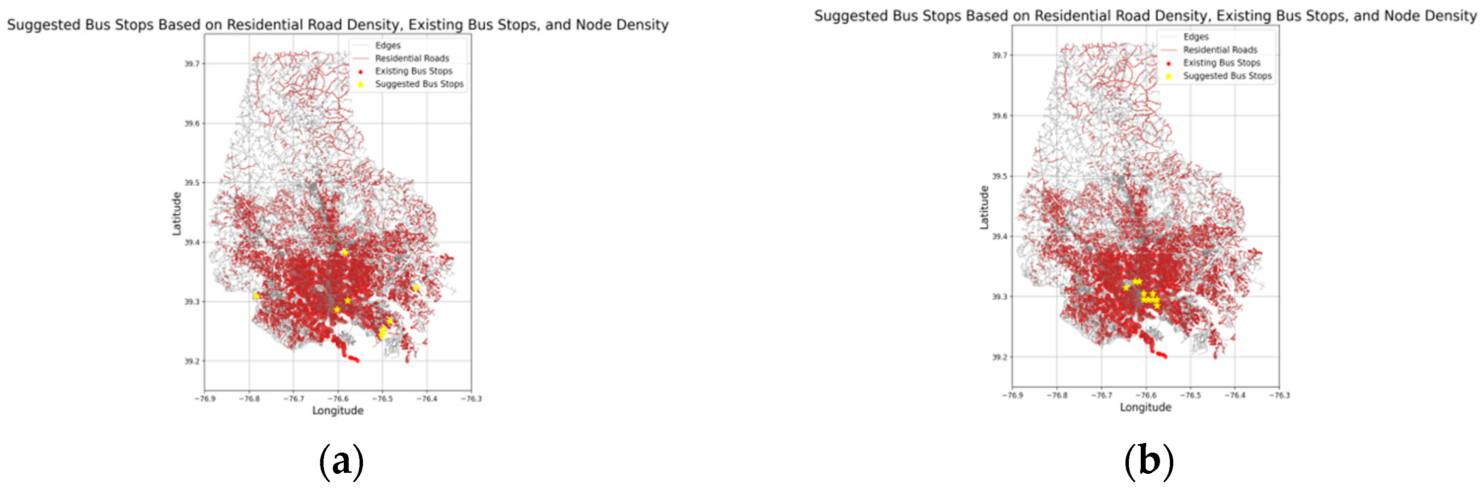
We used the second model to decide where to add new bus stops. By changing the value of GRID_SIZE (the size of each grid), we can adjust the accuracy of the result. The suggested bus stops to add are shown in Figure 13. The parameter of GRID_SIZE takes the value of 1 in the left diagram and takes the value of 10 in the left diagram.

We can see that as the accuracy of the chart increases, the locations that most require additional bus stations become more dispersed. This also indicates that the areas most in need of bus system coverage are not all in the city center. The bus company should consider adding routes to the suburbs to meet the commuting needs of suburban residents and their travel to the city center.

This may seem contrary to our previous finding that suburban route frequencies should be reduced, but that is not the case. What suburban routes need is not more frequent services, but more diverse route directions, because the population in the suburbs is not concentrated and the demand for bus rides may not be high, but the destinations are numerous. It is recommended to arrange more low-frequency suburban routes with different directions.

In conclusion, the bus system in Baltimore faces issues such as uneven route distribution and inefficient scheduling. Based on the model, we can observe the following impacts of adjusting the bus system:

• Increasing the frequency of commuting routes is beneficial for commuters to save time.
• Frequency decreasing in suburban routes may lead to a reduced likelihood of using public transportation in suburban areas.
• Proper adjusting can help save the expenditure of bus companies.

Different stakeholders are affected in the following ways:

• For commuters and urban residents, adjusting the bus frequency makes their daily commute and outings more convenient.
• For tourists, reducing the frequency of some less crowded routes may make it harder for them to catch a bus, which could cause some inconvenience, because not all the scenic spots are next to routes with many riders.
• For suburban residents, a more reasonable bus route arrangement will allow them to easily reach more places, rather than feeling convenient only when going downtown.

4.3. Optimization Network of Urban Road Traffic Systems

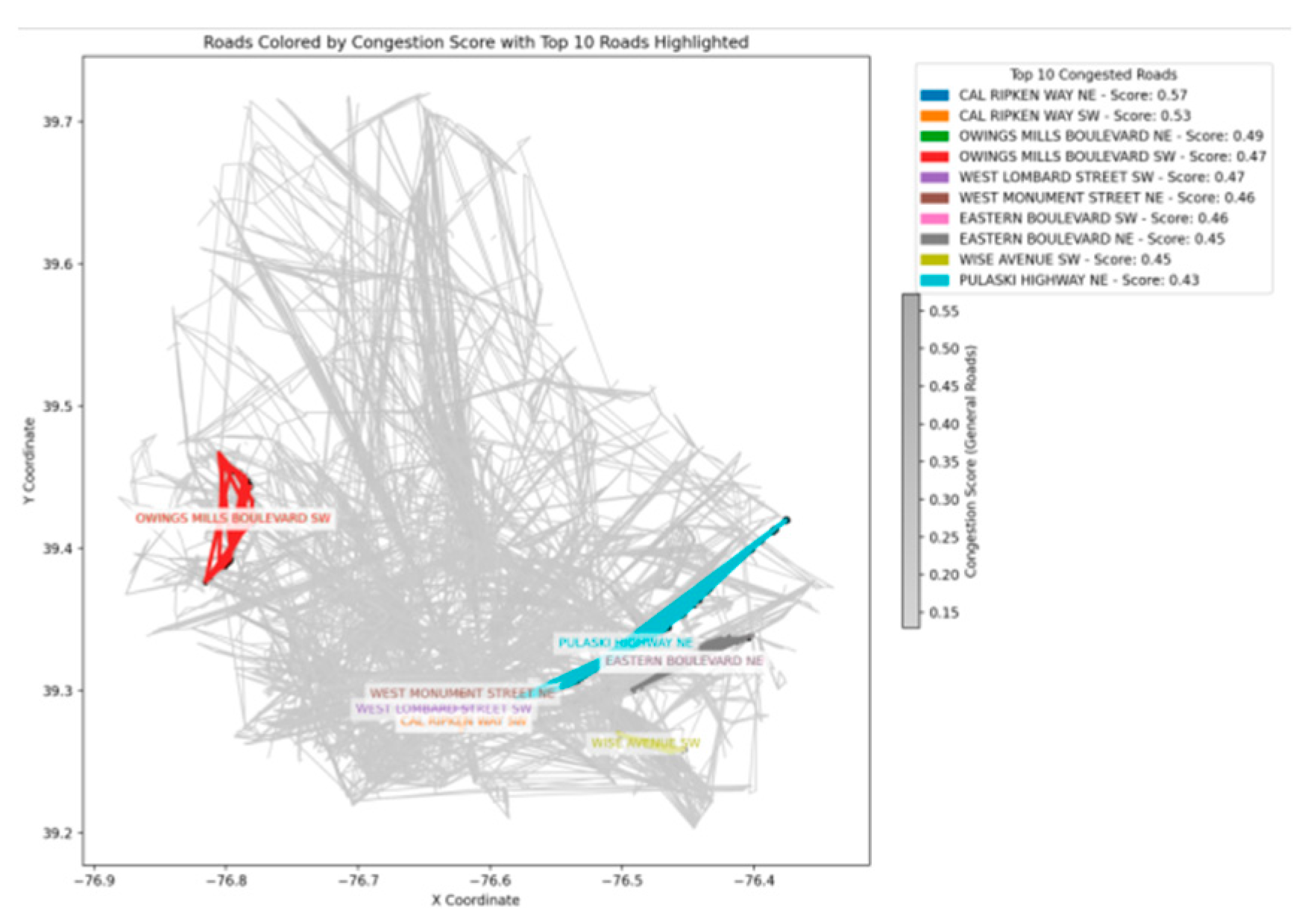
One of the characteristics of urban traffic is that the traffic flow in different directions on the same road can vary significantly. Initially, we will not consider the factors of the primary direction of flow. Under that assumption, the top 10 most congested roads ranked by our model are highlighted in Figure 14.

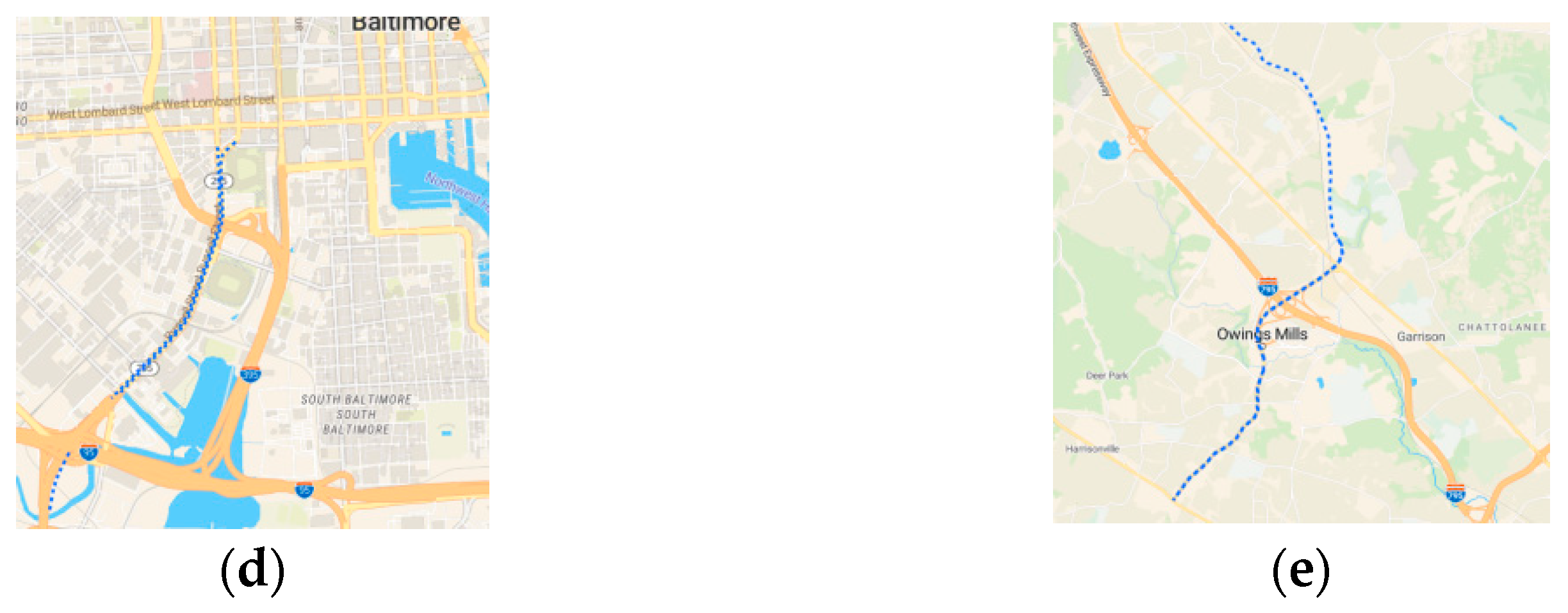
The figure shows several road segments in Baltimore with relatively high traffic flow. We hope to alleviate this situation through measures such as adding bus stops and constructing new roads. Below are the locations of some of these roads in OpenStreetMap (Figure 15). The map displays the entire road, but the actual high-traffic segments may only be parts of the road.

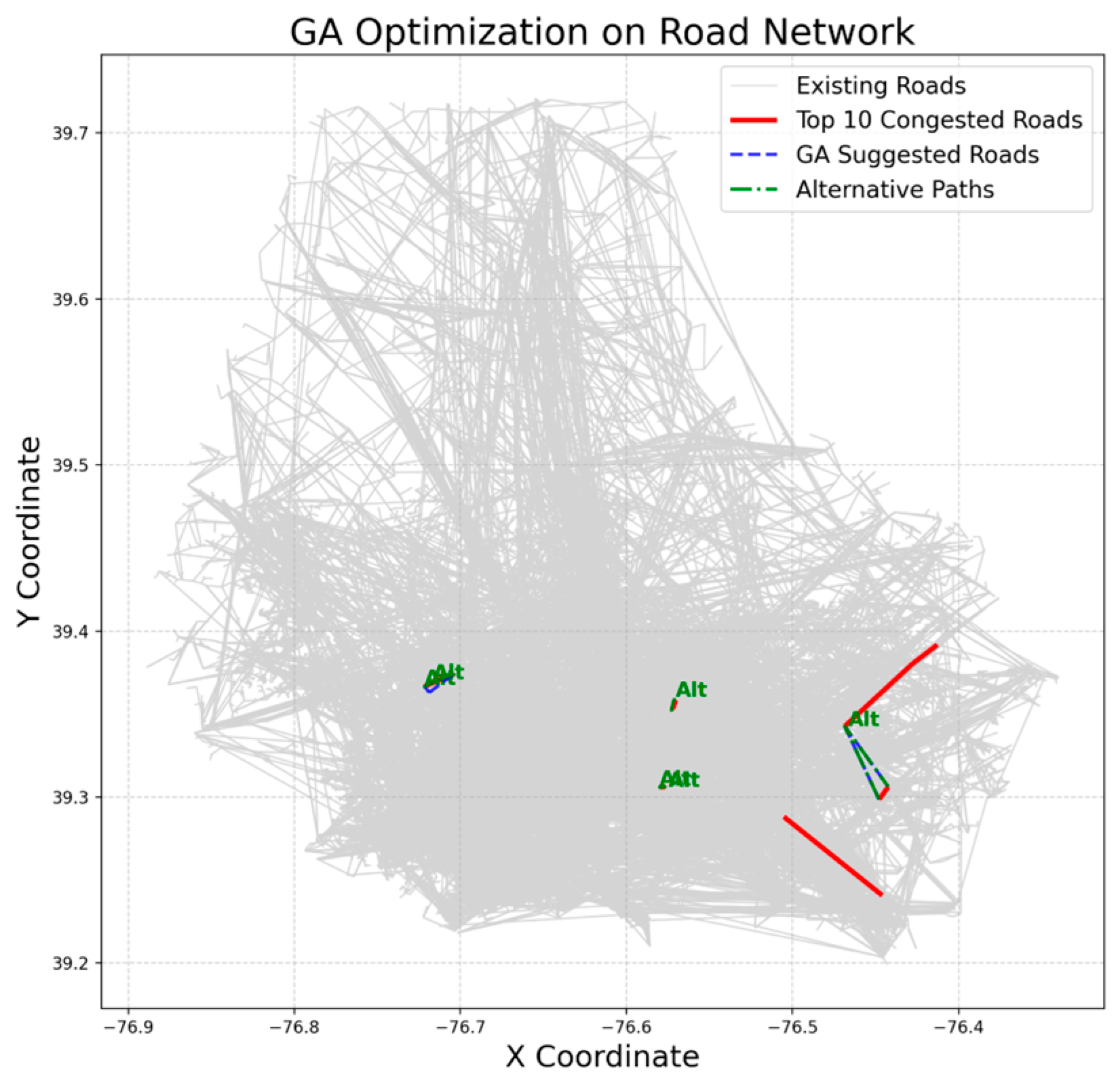
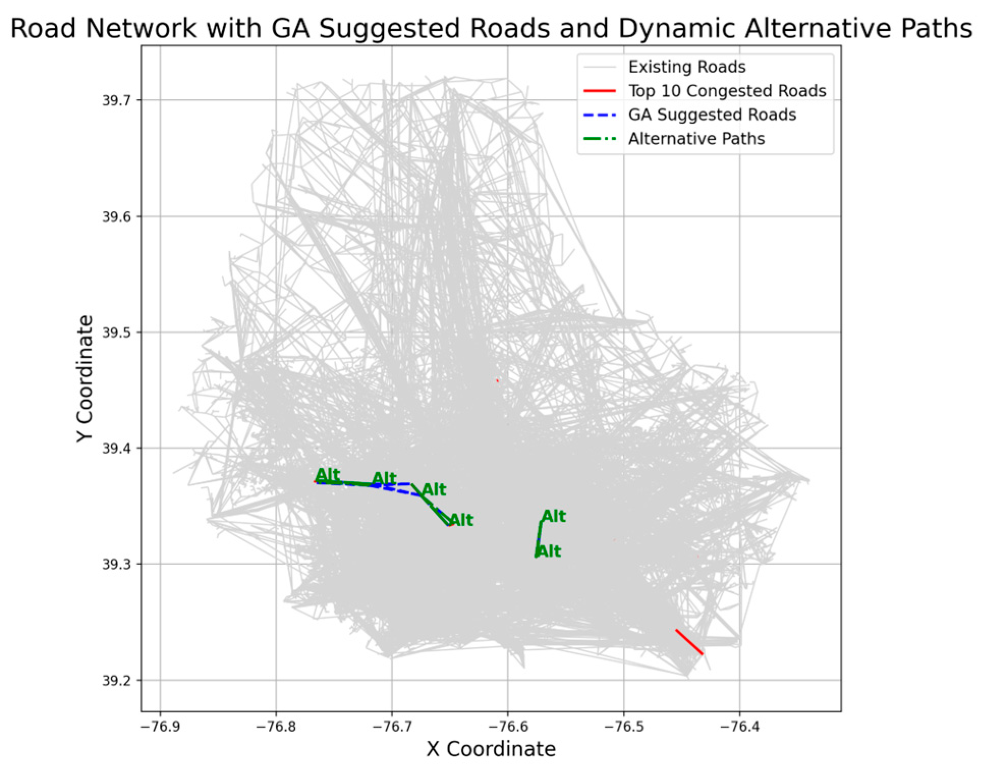
We considered the potential impact of constructing permanent infrastructure, so we used the method in Section 3.4 to choose the least possible road construction method that can alleviate traffic pressure to the greatest extent possible. Two of these roads connect the port to the southwest of the city (Cal Ripken Way, Windsor Mill Road), two connect the port to the northeast of the city (Eastern Boulevard, Windsor Mill Road), and one is located in the suburbs (Owings Mills Boulevard). Most of these roads are important arterial routes connecting downtown Baltimore, an important port city in the eastern United States, to the outside of the city. The model shows effective solutions for addressing the high traffic flow at these points, such as building new roads. It indicates that connecting Owings Mills Boulevard with other road segments, as well as connecting Cal Ripken Way and Windsor Mill Road, can help alleviate the traffic issues in these areas, as is shown in Figure 16. We try to divert the traffic flow of some relevant road sections, comprehensively consider the multi-stakeholder relationship, and increase the construction of some roads to alleviate the traffic pressure of the current important arterial roads, especially the traffic pressure and burden of the three roads of Owings Mills Boulevard, Eastern Boulevard, and Pulaski Highway, to ensure that passengers can enter Baltimore smoothly, that related goods can be transported from the port normally, and to ensure good traffic order and relieve traffic pressure.

If we take the direction of traffic flow into consideration, the result is similar but more accurate (Figure 17 and Figure 18).

From the two figures, we can observe that roads appeared here are also in the original figure (Figure 14). However, some roads only have one direction entering the top 10, such as Pulaski Highway, which only has the eastbound direction in the top 10. This indicates that this road handles a significant portion of the traffic demand for traveling from Baltimore to the northeast.

Additionally, the recommended new roads shown in Figure 18 have changed. A new suggested road has been added near Pulaski Highway on the east side of the city, indicating that this road could also help share the traffic load from the eastern suburbs.

This project will have the following significant impacts on local residents’ lives:

• It will resolve long-standing congestion issues on these road segments, improving travel speed.
• It will enhance the connectivity of the route network, reducing travel distance.
• Road construction in the urban area will cause significant noise and dust, leading to pollution.

It will also affect other stakeholders as follows:

• The construction of new roads will involve large-scale demolitions and generate considerable demand for real estate (especially between Cal Ripken Way and Windsor Mill Road, near the city center).
• Road construction in the urban area will cause significant noise and dust, leading to pollution.
• The government will need to allocate additional investments.
• Travelers and passthrough travelers will be less affected by traffic congestion (especially with the elimination of the traffic congestion on Owings Mills Boulevard in the suburbs).

The impacts of this process on other transportation demands and people’s lives are as follows:

• Private car users will experience reduced congestion due to the diversion caused by the new road.
• With more people willing to drive, there will be a reduction in the number of bus passengers, which will affect the bus companies’ decisions regarding the adjustment of bus frequency and routes.

5. Discussion

5.1. Discussion on Road Network Security

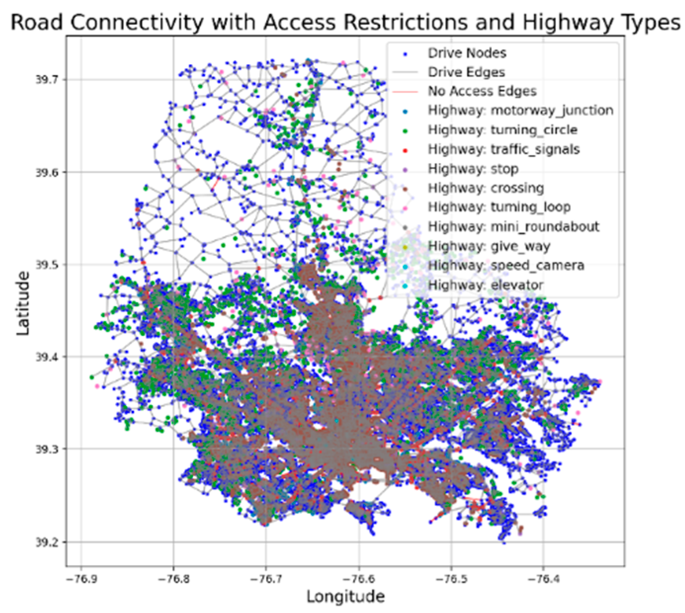
To further identify the sections where pedestrian safety should be enhanced, we also plotted the distribution map of traffic signal facilities in Baltimore. We should focus on strengthening pedestrian safety in areas with high traffic flow shown, but with a lack of traffic facilities as shown in Figure 19.

After reviewing and analyzing the data, we believe that the pedestrian safety problem in Baltimore may focus on the following aspects: the lack of proper infrastructure such as sidewalks, zebra crossings, and traffic lights on some roads, inadequate traffic signals causing risks for pedestrians crossing the street, and dangerous driving behaviors such as speeding, which aggravate the hidden danger of pedestrians.

To address pedestrian safety issues in Baltimore, the city government and relevant agencies have already taken a series of measures, such as implementing the “Toward Zero” initiative. We can also take the following measures to improve pedestrian travel safety.

a.

Improve Infrastructure Construction

Add sidewalks and crosswalks in lacking areas. Priority should be given to adding these facilities to ensure pedestrians have safe paths, especially in areas with high pedestrian traffic. Crosswalks should be more densely placed near schools, hospitals, and communities.

Construct pedestrian overpasses or underground passages. In areas with heavy traffic and concentrated pedestrian demand, such as commercial centers or transportation hubs, consideration should be given to building pedestrian overpasses or underground passages to reduce conflicts between pedestrians and vehicles.

b.

Optimize Traffic Signals and Signs

Set traffic signs properly. Place clear and explicit traffic signs at intersections and pedestrian crossing areas to remind drivers to pay attention to pedestrians. For example, set a “Slow Down and Yield” sign before crosswalks to remind drivers to slow down in advance and yield to pedestrians.

Adjust signal timing. Flexibly adjust the traffic signal timing based on actual traffic flow and pedestrian demand to ensure that both pedestrians and vehicles can pass through intersections safely and efficiently. For example, consider increasing the pedestrian green light time to reduce conflicts with right-turning vehicles.

These measures can effectively address the safety gaps in Baltimore’s pedestrian traffic system, improving pedestrian travel safety and convenience. Successfully implementing these measures may require the joint efforts of the government, communities, and citizens, involving multiple aspects such as infrastructure construction, traffic management, and safety education, to create a safer and more harmonious traffic environment.

5.2. Model Validity Analysis

5.2.1. The Impact of Emergencies on Urban Transport Networks: The Case of the Collapse of the Francis Scott Key Bridge

During the verification phase, we calculated the prediction relative error for each model on a per road for the year 2022 data. The calculation process is as follows: for a certain road, we first split the historical data into training data (2014–2021) and testing data (2022). Using the training data, we called on various models for one-step prediction to obtain the predicted values and then calculated the relative error. The calculation formula is as follows:

$$(\mathrm{P}\mathrm{r}\mathrm{e}\mathrm{d}\mathrm{i}\mathrm{c}\mathrm{t}\mathrm{e}\mathrm{d}\mathrm{ }\mathrm{V}\mathrm{a}\mathrm{l}\mathrm{u}\mathrm{e}\mathrm{ }–\mathrm{ }\mathrm{A}\mathrm{c}\mathrm{t}\mathrm{u}\mathrm{a}\mathrm{l}\mathrm{ }\mathrm{V}\mathrm{a}\mathrm{l}\mathrm{u}\mathrm{e})/\mathrm{A}\mathrm{c}\mathrm{t}\mathrm{u}\mathrm{a}\mathrm{l}\mathrm{ }\mathrm{V}\mathrm{a}\mathrm{l}\mathrm{u}\mathrm{e}$$

(18)

Subsequently, we took the absolute value of this relative error to obtain the model’s absolute relative error for that road and then squared each model’s error to obtain the squared error. After processing all the roads, for a certain model, we calculated the mean of the absolute relative errors across all roads, and multiplied by 100 to get the model’s Mean Absolute Percentage Error (MAPE) in the prediction of AADT or AAWDT, which represents the percentage of the average deviation from the true value; at the same time, we calculated the mean of the squared errors, multiplied by 10,000, to obtain the Mean Squared Percentage Error (MSPE), reflecting the degree of dispersion of the prediction relative error.

Table 5. Mean absolute percentage error and mean squared percentage error of AADT.

Model	Mean Absolute Percentage Error (MAPE)	Mean Squared Percentage Error (MSPE)
Polynomial Regression of degree 2	13.77	271.69
Support Vector Regression	8.72	385.39
Moving Average	7.44	292.38
Holt’s Linear Trend Method	6.93	198.17
Exponential Smoothing	6.40	193.23
Linear Regression	5.31	102.92
K-Nearest Neighbors	4.60	115.61
ARIMA	2.83	31.23

and

Table 6. Mean absolute percentage error and mean squared percentage error of AAWDT.

Model	Mean Absolute Percentage Error (MAPE)	Mean Squared Percentage Error (MSPE)
Polynomial Regression of degree 2	13.95	276.60
Support Vector Regression	9.04	382.91
Moving Average	7.61	288.22
Holt’s Linear Trend Method	7.29	173.36
Exponential Smoothing	6.57	170.16
Linear Regression	5.24	100.96
K-Nearest Neighbors	4.17	111.01
ARIMA	3.43	34.24

, respectively, show the prediction bias of different models under the AADT and AAWDT two indicators.

From Table 5 and Table 6, we can observe that the ARIMA model outperforms other models in predicting the Annual Average Daily Traffic (AADT) and Annual Average Weekly Day Traffic (AAWDT). Specifically, the ARIMA model has a MAPE value of 2.83 and an MSPE value of 31.23 when forecasting AADT, and a MAPE of 3.43 and an MSPE of 34.24 when predicting AAWDT. These values are the lowest among all listed models, indicating that the ARIMA model demonstrates favorable predictive accuracy for both metrics.

Compared to other models such as Exponential Smoothing, Holt’s Linear Trend Method, Moving Average, Linear Regression, Polynomial Regression of degree 2, Support Vector Regression, and K-Nearest Neighbors, the ARIMA model exhibits smaller predictive errors. For instance, the Polynomial Regression of degree 2 has a MAPE as high as 13.777 and an MSPE of 271.69 when predicting AADT, and an MAPE of 13.95 and MSPE of 276.60 when predicting AAWDT—significantly higher than the corresponding values of the ARIMA model.

The advantage of the ARIMA model lies in its ability to handle non-seasonal and seasonal components in time series data, capturing the dynamic characteristics of the data through autoregression, differencing, and moving average steps. This flexibility enables the ARIMA model to adapt to traffic flow data with complex patterns, providing more accurate forecast results. In contrast, other models may perform poorly when dealing with data that has a pronounced time dependency, leading to larger predictive errors.

Moreover, the low MAPE and MSPE values of the ARIMA model indicate its high stability and accuracy in predicting traffic flow. These characteristics of high precision and low error make the ARIMA model the preferred choice for traffic flow forecasting, especially in scenarios where high-precision predictions are needed to support traffic management and planning decisions. Thus, the ARIMA model’s superiority in predicting AADT and AAWDT is not only reflected in numerical values but also in its adaptability to time series data and practical application value.

5.2.2. Scenario 1: Public Transport Improvement Strategies for Urban Residents: Optimization of the Network of Urban Public Transport Systems

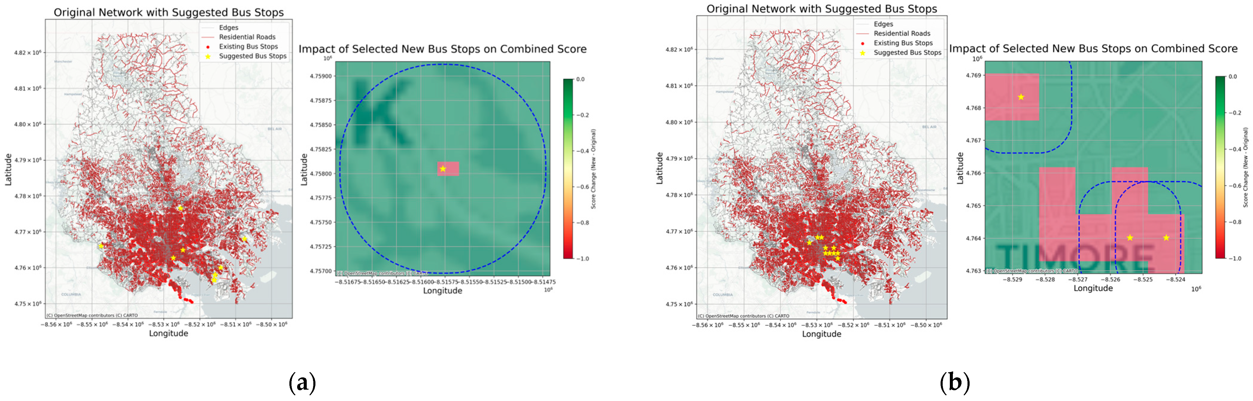
The effectiveness analysis of the new bus stop planning scheme is primarily reflected in the change of the composite scores after simulating the addition of new bus stops, and the impact on the local traffic network is demonstrated graphically. We first divide the area of interest into multiple small grids and count the number of residential roads, bus stops, and nodes within each grid, then calculate the composite score for each grid. Subsequently, we select the grids with the highest scores as the recommended locations for new bus stops and simulate the addition of a bus stop at these recommended locations, recalculating the composite scores for each grid and obtaining the score change values (score_change). In the visualization, the right subplot uses a buffer zone to display the range of influence, with color gradients intuitively reflecting the difference in composite scores before and after adding the bus stop, thereby assisting in assessing the effectiveness of adding bus stops in this area.

Before visualizing the data, the coordinates are all converted to the EPSG:3857 (Web Mercator) projection, mainly to overlay the actual map background, as the Web Mercator projection uses meters as the unit, while the WGS84 (EPSG:4326) coordinates are in degrees of longitude and latitude. In the converted map, the units of both the vertical and horizontal axes are meters, reflecting the actual planar distance under the Web Mercator projection. Although the latitude and longitude coordinates labeled on the map are in degrees before conversion, after the conversion, and overlay with the base map, the x-axis represents the horizontal distance (approximately east–west), and the y-axis represents the vertical distance (approximately north–south), thus allowing the distances and ranges on the map to be compared with the actual geographical locations, facilitating the evaluation of the impact of new bus stops on the surrounding traffic structure. (Due to the scattered distribution of new stations, we have chosen to display only a selection of stops in Figure 20).

In Figure 20, we can observe that the addition of new bus stops can effectively alleviate traffic congestion in the local community to a certain extent, leading to satisfactory improvements. This provides guidance and convenience for public travel and, when combined with actual maps, can offer precise recommendations for subsequent urban transportation planning.

5.2.3. Scenario 2: Road Traffic Improvement Strategies for Urban Residents: Optimization Network of Urban Road Traffic Systems

We conducted simulation experiments under the condition of increased pathways to verify the effectiveness of the current model. Initially, the genetic algorithm (GA) was utilized to generate a set of new road schemes, which were then assessed for their impact on existing congested sections using network path analysis. After establishing the base road network, we calculated the number of alternative paths for the top 10 most congested road segments (ranked based on comprehensive congestion scores). The number of alternative paths was determined by calling relevant functions in the networkX library, which counted the number of simple paths between each pair of nodes. This number reflects the available options within the existing network for a given road segment.

Following the selection and addition of new roads into the network by GA, we recalculated the number of alternative paths for the same set of target road segments. The key metric for validation was the difference between the number of alternative paths obtained in the base network and those after the addition of new roads. This difference reflects the degree of improvement the new roads provided in alleviating the target congested sections; the larger the improvement value, the more alternative paths are available, and the better the congestion relief effect. In addition to displaying the improvement value for each road segment, the code also calculated the average improvement value for all target road segments. This average value serves as a quantitative indicator of the overall optimization effect, intuitively reflecting the contribution of the new road network to congestion relief.

From Figure 21a, we can observe that without considering the direction, the new planned paths have shown significant effectiveness in alleviating congestion. In particular, for CAL RIPKEN WAY and RUSSELL STREET, the number of new planned paths increased from one to four, which is a substantial improvement. Similarly, the number of new planned paths for OWINGS MILLS BOULEVARD increased from two to four, and HILTON PARKWAY, HONEYGO BOULEVARD, and WINDSOR MILL ROAD also saw an increase of two new planned paths, indicating that the new planned paths have a significant alleviating effect on the congestion issues of these roads. However, for EASTERN BOULEVARD and WISE AVENUE, the number of new planned paths did not increase significantly, suggesting that the new planned paths have limited alleviating effect on the congestion issues of these roads (or they have achieved indirect diversion of other paths).

In Figure 21b, when considering the direction, the alleviating effect of the new planned paths on congested roads varies. The number of new planned paths for the PULASKI HIGHWAY (NE) increased from one to five, showing that the new planned paths have a significant alleviating effect on the congestion issues of this road. CAL RIPKEN WAY (SW), CAL RIPKEN WAY (NE), OWINGS MILLS BOULEVARD (SW), and OWINGS MILLS BOULEVARD (NE) also saw their new planned paths increase from one to three, from one to three, from one to two, and from two to three respectively, indicating that the new planned paths also have some alleviating effect on the congestion issues of these roads. However, the number of new planned paths for EASTERN BOULEVARD and WEST MONUMENT STREET (NE) did not increase, suggesting that when considering the direction, the new planned paths have limited alleviating effect on the congestion issues of these roads (or they have achieved indirect diversion of other paths).

Overall, the new planned paths have shown positive effects in alleviating traffic congestion on certain specific roads and have shown obvious congestion-alleviating effects in certain directions. This indicates that when planning traffic and designing roads, it is necessary to consider the specific needs and traffic flow distribution of different roads more carefully, and how to allocate traffic flow most effectively through the new planned paths. Future planning work may require more refined design and a deeper analysis of the existing road network and traffic patterns to ensure that the new planned paths can alleviate traffic congestion more comprehensively.

5.3. Strengths and Shortcomings of the Models

5.3.1. Strengths

In Section 4.1, the ARIMA model was applied to analyze the annual average daily traffic and annual average weekday traffic data for Baltimore, under the assumption that the bridge has not collapsed. This assumption improves the reliability of the data by ensuring that the observed traffic patterns are not influenced by a structural failure.

The ARIMA model, as used in Section 3.2, is capable of handling non-stationary time series data. By applying differencing to make the data stationary, it allows for more robust modeling and accurate forecasting of traffic behavior over time.

In Section 3.3, the strategy was not limited to increasing the number and frequency of buses on certain routes; new bus stations were also added to fill gaps in existing bus routes. This dual approach helps alleviate bus pressure in high-traffic areas and improves overall accessibility.

Furthermore, the PCA method employed in Section 3.3 and Section 3.4 effectively reduces the dimensionality of high-dimensional datasets by extracting the main components. This process amplifies the influence of key factors on the outcome, thereby enhancing the reliability of the data for subsequent analysis.

Finally, by comprehensively considering the effects of multiple indicators on Baltimore’s traffic flow in Section 3.3 and Section 3.4, a multi-factor analysis was performed that improves predictive accuracy. This comprehensive approach not only better informs the bus station construction plan but also provides a clearer understanding of the congestion situation on the roads of Baltimore.

5.3.2. Shortcomings

The ARIMA model assumes linear relationships between time series data, so if there are non-linear interactions between AADT and AAWDT in Baltimore, its predictions may be inaccurate. Moreover, since ARIMA is designed for univariate time series, it cannot directly handle multiple factors—such as road width and speed limits—without switching to a multi-variate approach like VAR.

Similarly, PCA assumes that the data is linearly distributed. When facing non-linear factors (for example, Rider_On in Section 3.3 or D-Factor and K-Factor in Section 3.4), PCA might not effectively reduce the dimensionality. In addition, since PCA extracts principal components via the covariance matrix, the presence of outliers in large traffic datasets can exaggerate the variances in certain directions, potentially distorting the true structure. Furthermore, using six indicators in Section 3.4 might lead to some information loss if too many principal components are retained.

The grid-based segmentation model in Section 3.3 places new bus stations at the center of each grid cell, neglecting important internal variations within the grid. Also, if the grid boundary width is set to 0.001 m, the resulting statistics could be imprecise, thereby affecting the accuracy of the bus station locations.

5.3.3. Optimizing Models

In Section 3.2, to further enhance prediction accuracy, more detailed road information can be incorporated into forecasting models. For instance, including supplementary data such as the number of lanes and lane directions can provide additional predictive reference indicators for Baltimore’s annual average daily traffic and annual average weekday traffic. This enriched dataset would more accurately capture the characteristics of different road segments and lead to improved forecasting performance.

In Section 3.3 and Section 3.4, prediction accuracy can be further improved by incorporating data from various types of nodes, such as road intersections, highway interchanges, and pedestrian crossings. Analyzing these diverse node types allows the model to capture a broader range of traffic behaviors, resulting in more comprehensive recommendations for bus scheduling and road planning.

In Section 5.1, the focus can be expanded beyond pedestrian safety to include a wider array of traffic safety issues. By analyzing historical data on motor vehicle accidents and incidents involving both non-motorized vehicles and motor vehicles, it is possible to generate accident heat maps that identify areas with a high density of accidents. This approach would enable targeted traffic safety measures in accident-prone zones, thereby creating a more comprehensive and resilient traffic safety system.

5.4. Discussion on the Specific Implementation of the Plan

In this section, we will discuss the financial, legal, and social aspects related to the implementation of the proposed intelligent traffic network model. Implementing an intelligent traffic network model requires substantial initial investment, including the construction of infrastructure, the procurement and installation of intelligent traffic management systems, and the upgrading of related technologies. These initial costs may put pressure on the city’s budget. However, in the long run, the intelligent traffic network can improve traffic efficiency, reduce congestion, thereby reducing economic losses caused by traffic delays. Moreover, the intelligent traffic system can decrease traffic accidents, lowering medical and insurance costs. Therefore, despite the significant initial investment, the costs can be recouped and economic benefits can be generated in the long term by increasing traffic efficiency and reducing accidents. To ensure the financial feasibility of the project, it is recommended to conduct a detailed cost–benefit analysis to assess the economic returns of different investment plans, while also considering ways to share costs through public–private partnerships or government subsidies.

The implementation of the current intelligent traffic network must comply with relevant laws and regulations, including data protection, privacy rights, intellectual property, and public safety. For instance, when using traffic monitoring data, it is essential to adhere to data protection regulations to safeguard personal privacy. Additionally, the deployment of intelligent traffic systems may require approval and permits from relevant departments. Therefore, during the project planning phase, collaboration with legal advisors is necessary to ensure all implementation steps meet legal requirements and avoid potential legal disputes in the future. At the same time, it is also necessary to consider how to support the development of intelligent traffic systems through legislation, such as by enacting regulations to promote data sharing and standardization of intelligent traffic technologies.

The implementation of the intelligent traffic network may have profound social impacts. On one hand, it can enhance traffic efficiency, reduce congestion, and lower accident rates, thereby improving the quality of life for residents. On the other hand, the implementation of intelligent traffic systems may lead to social inequality; for example, if intelligent traffic services are concentrated in affluent areas, it may exacerbate the unequal distribution of social resources. Furthermore, the implementation of intelligent traffic systems may impact certain industries, such as reducing the demand for traditional traffic management personnel, thereby affecting employment. Therefore, when implementing the intelligent traffic network, a social impact assessment is needed to ensure the fairness and inclusiveness of the solutions and to minimize the negative impact on society. At the same time, educational and training programs are also required to help affected groups adapt to new technologies and reduce the risk of unemployment.

Additionally, to effectively translate the proposed intelligent traffic network model into practice, a detailed implementation strategy needs to be formulated. This includes determining the stages and steps of implementation, clarifying the responsibilities and roles of all parties, and establishing inter-departmental cooperation mechanisms. Firstly, detailed project planning is required, including technology selection, system design, and implementation plans. Secondly, a project management team needs to be established to be responsible for the execution and supervision of the project. Moreover, cooperation with traffic management departments, technology suppliers, community organizations, and other stakeholders is necessary to ensure the smooth implementation of the project. During the implementation process, regular project progress assessments are also needed, and the implementation strategy should be adjusted according to the actual situation.

6. Conclusions

This paper uses the ARIMA algorithm to comprehensively predict and analyze the impact of the collapse or reconstruction of the Francis Scott Key Bridge on traffic flow. Considering the interests of multiple stakeholders, we propose an intelligent bus network model based on increasing bus stations and adjusting the number and frequency of buses on corresponding bus routes, using principal component analysis and grid segmentation methods. Additionally, we present a comprehensive traffic network model for road expansion and improvement, based on principal component analysis, genetic algorithms, and KD-tree, to analyze total and bidirectional traffic flow. At the same time, considering traffic safety, we analyze safety from multiple perspectives, including accident-prone areas and traffic signal intersections, and provide corresponding recommendations. This study provides Baltimore with an intelligent traffic network model and also offers references for road traffic issues in other cities, helping to promote the construction and development of smart transportation cities.