Intelligent Resource Allocation for Task-Sensitive Autonomous Vehicular Systems

Abstract

This paper addresses the resource allocation challenges in autonomous vehicle (AV) networks for delay-sensitive perception tasks. Current vehicular networks face sub-optimal resource distribution and excessive communication overhead, hindering the performance of AVs. We propose an integrated approach that combines a platoon-based system model with optimization techniques using Deep Q-Networks (DQN) and Particle Swarm Optimization (PSO). The platoon-based model enables AVs to share resources effectively, while the DQN and PSO models optimize task offloading and reduce overhead. Simulation results across various traffic scenarios demonstrate that the PSO algorithm outperforms traditional methods in task completion rates, overhead minimization, and platoon formation. This approach offers a significant advancement in enhancing AV network performance and ensuring timely task execution.

1. Introduction

The rapid advancements in autonomous driving technology have the potential to significantly enhance transportation systems, offering improvements in safety, efficiency, and environmental sustainability [1]. Autonomous vehicles (AVs), which operate without human intervention, rely heavily on complex communication and computing systems to make real-time decisions, navigate roads, and perform essential tasks such as object detection, lane-keeping, and collision avoidance. Recent breakthroughs in integrated sensing and communication (ISAC) technologies, such as terahertz-band transceivers for UAVs in 6G networks [2], further expand the capabilities of vehicular networks by enabling ultra-high-speed data exchange and precise environmental sensing. While these advancements address bandwidth and latency challenges, they simultaneously intensify the demand for intelligent resource allocation to fully leverage such high-performance infrastructure.

Despite the tremendous promise of AVs, several challenges remain, particularly in the realm of communication and resource management [3]. A key issue in current vehicular networks is the resource allocation problem, which arises when AVs need to process and exchange vast amounts of data from onboard sensors in real time [4]. These tasks, such as sensor fusion and perception processing, are highly delay-sensitive. A delay in processing or communication could result in inaccurate data, jeopardizing the safety and performance of the AV. Furthermore, inefficient resource allocation among AVs, Road-Side Units (RSUs), and Edge Computing Devices (ECDs) often leads to underutilization of computational resources or excessive overhead, hindering the overall performance of the system [5].

As the number of AVs on the road increases, the demands on the communication infrastructure, including RSUs and ECDs, will intensify. The existing infrastructure struggles to meet the growing demands for real-time data processing and communication, especially in areas with high vehicle density, such as urban environments during peak hours [6,7]. These areas suffer from limited communication bandwidth and computational capacity, leading to delays and increased risk of failure in performing critical tasks. This inefficiency is further compounded by high communication overheads, which reduce the effective use of available resources and delay the execution of tasks within the strict time constraints required for AV operation.

To address these challenges, this paper proposes a novel approach that integrates a platoon-based approach with advanced resource optimization techniques. In the proposed model, AVs within a platoon can cooperate by sharing resources and offloading tasks to more capable vehicles or ECDs when necessary. This collaborative driving approach is an effective strategy to improve resource utilization and reduce the computational burden on individual vehicles. Furthermore, the paper introduces two Overhead Optimization Models—one based on Deep Q-Networks (DQNs) and the other based on Particle Swarm Optimization (PSO). Both models aim to optimize the allocation of communication and computing resources, ensuring the timely execution of perception tasks while minimizing system overhead.

The DQN-based approach leverages the power of deep reinforcement learning to continuously adapt and learn optimal task-offloading strategies [8,9,10]. The PSO-based model, inspired by swarm intelligence, seeks the best solution by simulating the behavior of a group of particles [11,12]. Both models are designed to handle the dynamic and complex nature of vehicular networks, where resources and task priorities vary over time. Through extensive simulations under different traffic conditions, we demonstrate the superiority of the proposed models in reducing system overhead, increasing task completion rates, and improving platoon formation efficiency compared to traditional methods.

This work contributes to the growing body of research on autonomous vehicular networks by providing a robust and scalable solution to resource allocation and task execution in delay-sensitive environments. The proposed platoon-based approach not only enhances the performance of AV networks but also ensures the efficient use of available resources, enabling the safe and effective deployment of AVs in real-world scenarios. In addition, by addressing the communication and computing overhead challenges, this study lays the groundwork for future advancements in autonomous driving systems and the development of smart transportation networks. The main contributions are listed as follows.

• Platoon-based Approach: A platoon-based approach is introduced, where AVs can cooperate and share resources within platoons. This reduces the computational burden on individual vehicles and optimizes task execution.
• Joint Optimization through DQN and PSO: A combined optimization approach based on Deep Q-Networks (DQNs) and Particle Swarm Optimization (PSO) is developed. This approach minimizes communication and computing overheads in AV networks, ensuring efficient task offloading and resource allocation.
• Significant Performance Improvement: Extensive simulations demonstrate that the proposed models significantly improve system performance. They achieve higher task completion rates, reduce overhead, and enhance platoon formation efficiency, outperforming traditional methods.

The remainder of this paper is organized as follows. Section 2 presents the system model, including the physical entities, platoon-based approach, and digital twin model. Section 3 introduces the Overhead Optimization Model Based on DQN, detailing how it optimizes task offloading and resource allocation. Section 4 describes the Overhead Optimization using PSO for DQN Model, which minimizes system overhead using swarm intelligence. Section 5 presents the simulation results, compares the performance of the proposed models, and analyzes their effectiveness under various traffic conditions. Finally, Section 6 concludes the paper, summarizing the findings and suggesting potential future research directions.

2. System Model

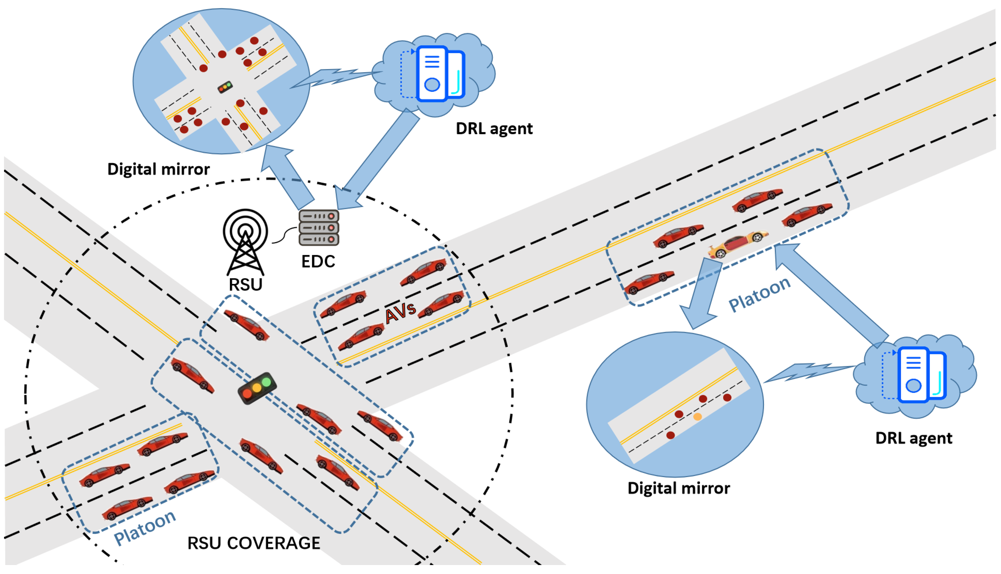
In the autonomous driving domain, an efficient system model is of utmost significance for the seamless operation of vehicles [13]. The presented system model, which incorporates platoons, offers a more sophisticated approach to vehicle-to-infrastructure (V2I) and vehicle-to-vehicle (V2V) interactions. It is composed of two main layers in Figure 1: the physical entities layer and the digital twin layer.

Autonomous vehicles (AVs) lie at the core of the physical entities layer. Each AV is outfitted with an on-board unit (OBU) that enables communication with Road-Side Units (RSUs) and other AVs. When within the coverage of RSUs, AVs can utilize the connected Edge Computing Devices (ECDs) for computational assistance [14]. ECDs, boasting substantial computing resources, are capable of handling computationally intensive tasks offloaded by AVs, thereby enhancing the driving efficiency and safety of individual AVs [15]. In regions with limited RSU coverage, the formation of platoons becomes a critical mechanism. A platoon is a collaborative driving group consisting of multiple AVs, where vehicles communicate via V2V technology [16,17]. The speed s and direction $\alpha$ of vehicles are decisive factors in platoon formation. Vehicles with similar speeds and directions are more prone to forming a platoon. For example, if several AVs are traveling along the same route with speeds within a certain range, they can band together to form a platoon. This not only minimizes the communication overhead caused by relative motion but also facilitates more efficient resource sharing. In a platoon, vehicles assume distinct roles. The lead vehicle is responsible for guiding the platoon, making driving decisions based on its sensor data and the overall platoon situation [18]. It determines which tasks to execute locally and which to offload to ECDs (if available). The member vehicles follow the lead vehicle’s decisions and relay their driving-related information. This coordinated movement optimizes the driving process and alleviates the computational burden on each AV.

The twin digital layer supplements the layer of physical entities [19]. Each AV has a corresponding digital twin (DT) deployed on the connected ECD. The DT, acting as a virtual replica of the physical AV, continuously gathers real-time information about the vehicle, such as speed, direction, and computational resource status. This information is utilized to precisely simulate the vehicle’s state in the virtual environment. DTs play a crucial role in decision-making. They interact with each other on the virtual network to optimize driving strategies for physical AVs [20]. When a vehicle in a platoon experiences a sudden change in speed or direction, its DT promptly updates the virtual model and shares the updated information with other DTs. Through such interactions, DTs can jointly re-evaluate driving decisions, such as adjusting task allocation among vehicles, ensuring that the platoon can adapt to changes in the driving environment in a timely manner and maintain its stability and safety [21,22].

The following

Table 1. System model parameters.

Symbol	Description
V	Set of autonomous vehicles (AVs)
B	Set of cellular base stations (CBSs)
$E_{b_n}$	Edge Computing Device at CBS $b_n$
s	Speed of an AV
$\alpha$	Direction of an AV
$T_{v_{gp},b_n}$	Transmission rate between AV $v_{gp}$ and CBS $b_n$ (Mbps)
$T_{v_{gp},v_{g^{\prime }p}}$	Transmission rate between AVs $v_{gp}$ and $v_{g^{\prime }p}$ (Mbps)
${\gamma }_{v_{gp},b_n}$	Unit-time transmission cost between AV $v_{gp}$ and CBS $b_n$
${\gamma }_{v_{gp},v_{g^{\prime }p}}$	Unit-time transmission cost between AVs $v_{gp}$ and $v_{g^{\prime }p}$
$C_{v_{gp}}$	Computing capacity of AV $v_{gp}$ (GHz)
$C_{E_{b_n}}$	Computing capacity of ECD $E_{b_n}$ (GHz)
$P_{v_{gp}}$	Unit cost of computing on AV $v_{gp}$ (per GHz·s)
$P_{E_{b_n}}$	Unit cost of computing on ECD $E_{b_n}$ (per GHz·s)
$d_q$	Data size of task $d_q$ (MB)
$c_q$	Required computing resources of task $d_q$ (GHz·s)
${\tau }_q$	Execution deadline of task $d_q$ (seconds)
$D_{v_{gp}}^{b_n}$	Tasks offloaded by $v_{gp}$ to CBS $b_n$
$D_{v_{gp}}^{v_{g^{\prime }p}}$	Tasks offloaded by $v_{gp}$ to AV $v_{g^{\prime }p}$
$D_{v_{gp}}^{\mathrm{local}}$	Tasks executed locally by AV $v_{gp}$
$D_{b_n}^{\mathrm{edge}}$	Tasks executed by edge device $E_{b_n}$
$O_{\mathrm{com}}$	Total communication overhead
$O_{\mathrm{comp}}$	Total computing overhead
O	Total system overhead ($O_{\mathrm{com}}+O_{\mathrm{comp}}$)

summarizes the key parameters used in the system model:

2.1. CBSs and ECDs

In the Autonomous Vehicular Networks (AVNs), the set of road segments is denoted as $\mathcal{R}=\{r_1,\dots ,r_m,\dots ,r_M\}$. Along each road segment $r_m(m\in \mathcal{R})$, multiple Cellular Base Stations (CBSs) are deployed and interconnected via high-speed wired links. Let $\mathcal{B}=\{b_1,\dots ,b_n,\dots ,b_N\}$ be the set of CBSs on road segment $r_m$ in the AVNs, and the set of driving groups within the coverage of CBS $b_n$ be $\mathcal{G}=\{g_1,\dots ,g_p,\dots ,g_P\}$. CBS $b_n$ provides various vehicular services to Autonomous Vehicles (AVs) within its communication range through wireless connections. For an AV $v_{g_p}$ in group $g_p$, the transmission rate between it and the connected CBS $b_n$ is $T_{v_{g_p},b_n}$, and the cost per unit time for data delivery is ${\gamma }_{v_{g_p},b_n}$. Each CBS is equipped with an Edge Computing Device (ECD) to support autonomous driving. Denote the ECD at CBS $b_n$ as $E_{b_n}$. The computing resources of $E_{b_n}$ and its declared price per unit time are $C_{E_{b_n}}$ and $P_{E_{b_n}}$, respectively. Additionally, $E_{b_n}$ has a database that stores all historical tasks $\mathcal{T}=\{t_1,\dots ,t_q,\dots ,t_Q\}$ and records the average number of tasks $\overline{T}$ that each AV or collaborative driving group needs to complete when passing through this road segment.

2.2. AVs and Platoons

Let the transmission rate between AVs $v_{g_p}$ and $v_{g_p^{\prime }}$ be $T_{v_{g_p},v_{g_p^{\prime }}}$ and the cost per unit time for data delivery be ${\gamma }_{v_{g_p},v_{g_p^{\prime }}}$. Each AV has computing resources $C_{v_{g_p}}$ and a declared price per unit time $P_{v_{g_p}}$, and generally $C_{v_{g_p}}<C_{E_{b_n}}$. Thus, AVs can offload some tasks to the connected ECD based on their resources and task requirements. In a platoon, there are two types of vehicles: the lead vehicle and the member vehicles. The lead vehicle is responsible for leading the platoon. It decides which tasks to execute locally and which to offload to the ECD according to its resources. Member vehicles follow the driving decisions of the lead vehicle and pass their own driving decisions to the next vehicle. When a vehicle joins a platoon, it considers factors such as the compatibility of its speed and direction with the platoon, as well as the potential reduction in costs. For instance, if joining a platoon can help a vehicle reduce its computing and transmission costs through resource sharing and cooperation, it will be more inclined to join.

2.3. Task Model

During autonomous driving, AVs must complete a variety of computationally intensive and delay-sensitive tasks. Each task $d_q$ is characterized by its data size $d_q$, required computing resources $c_q$, and execution deadline ${\tau }_q$. If an AV can complete a task locally within the deadline using its own computing capacity, it executes the task directly; otherwise, the task is offloaded to an ECD or other AVs. In the context of platoons, task allocation and execution are determined not only by the resources and capabilities of individual AVs but also by the overall resource coordination and task priorities within the platoon. For urgent and resource-intensive tasks, the platoon may prioritize the assignment to AVs with stronger computing capabilities or use the collaborative computing of multiple vehicles to ensure task completion within the deadline, thus guaranteeing driving safety and efficiency.

2.4. Digital Twin Model

In the AVNs, each AV $v_{g_p}$ has a corresponding digital twin (DT) ${\tilde{v}}_{g_p}$. The DT is deployed on the ECD connected to the AV and serves as a digital representation of the AV in the virtual network, facilitating decision-making for the AV in the physical network. The DT ${\tilde{v}}_{g_p}$ has access to the AV’s parameters such as $C_{v_{g_p}}$ and $P_{v_{g_p}}$, and the AV can upload its information to the DT. Each AV creates a virtual account in its DT for transactions in the AVNs. When an AV leaves the communication range of $E_{b_n}(n\in \mathcal{B})$ and enters that of $E_{b_{n^{\prime }}}(n^{\prime }\in \mathcal{B},n^{\prime }\ne n)$, the DT is transferred from $E_{b_n}$ to $E_{b_{n^{\prime }}}$ via high-speed wired links in advance. In the platoon scenario, the DT also needs to obtain real-time information about the vehicle’s speed s and direction $\alpha$ to accurately simulate the vehicle’s state and predict its trajectory. Based on this information, the DT can interact with other DTs on behalf of the AV to make driving decisions. When an AV leaves the original road segment $r_m$ and moves to a new road segment $r_{m^{*}}$, the DT ${\tilde{v}}_{g_p}$ settles the cost of $v_{g_p}$ in the original road segment $r_m$ through its virtual account. During platoon driving, if the speed or direction of a vehicle in the platoon changes suddenly, the DT will re-evaluate the task assignment and collaboration strategy to optimize the overall driving cost and efficiency of the platoon, ensuring its stability and safety.

3. Overhead Optimization Model Based on DQN

3.1. Problem Formulation

In the platoon-based autonomous vehicle system, the primary objective is to minimize the overall overhead O, which encompasses two key components: the communication overhead $O_{com}$ and the computing overhead $O_{comp}$.

The communication overhead is calculated as the sum of transmission time multiplied by cost per unit time:

$$O_{\mathrm{com}}=\sum _{v_{gp}\in V}\sum _{b_n\in B}\left(\sum _{d_q\in D_{v_{gp}}^{b_n}}{\displaystyle \frac{d_q}{T_{v_{gp},b_n}}}·{\gamma }_{v_{gp},b_n}\right)+\sum _{v_{gp}\in V}\sum _{v_{g^{\prime }p}\in V}\left(\sum _{d_q\in D_{v_{gp}}^{v_{g^{\prime }p}}}{\displaystyle \frac{d_q}{T_{v_{gp},v_{g^{\prime }p}}}}·{\gamma }_{v_{gp},v_{g^{\prime }p}}\right)$$

(1)

where $\mathcal{V}$ represents the set of all autonomous vehicles (AVs) in the system.

The computing overhead is calculated based on the actual computational resources required by tasks and the unit cost of processing on either the AV or the ECD:

$$O_{\mathrm{comp}}=\sum _{v_{gp}\in V}\sum _{d_q\in D_{v_{gp}}^{\mathrm{local}}}{c}_q·P_{v_{gp}}+\sum _{b_n\in B}\sum _{d_q\in D_{b_n}^{\mathrm{edge}}}{c}_q·P_{E_{b_n}}$$

(2)

For a task $d_q$ executed locally by an AV or offloaded to an edge device, the cost is given by $c_q·P$, where P is the unit price of computing resources at the executing entity.

The total overhead $O=O_{com}+O_{comp}$. Our goal is to discover an optimal task-offloading and platoon-formation strategy to minimize O, while adhering to constraints such as task deadlines ${\tau }_{t_q}$ and available computing resources $C_{v_{g_p}}$ and $C_{E_{b_n}}$.

3.2. Deep Q-Network (DQN) Model Based on Markov Process

We formulated the overhead optimization problem as a Markov Decision Process (MDP). An MDP is defined by a tuple $(S, A, P, R, \gamma )$, where S represents the state space, A is the action space, P is the state-transition probability function, R is the reward function, and $\gamma$ is the discount factor.

3.2.1. State Space (S)

The state of the system at time step t, denoted as a vector $s_t$, encompasses comprehensive information about the autonomous vehicles (AVs) and the overall network environment. It includes the AVs’ speeds s, which can impact communication stability and task execution time due to relative motion. The directions $\alpha$ are also crucial, as they determine the possibility of vehicles forming platoons; vehicles with similar directions are more likely to cooperate. The remaining computing resources $C_{v_{sp}}$ of each AV are essential for evaluating its ability to handle tasks locally. Additionally, the status of tasks $t_q$ is incorporated, indicating whether a task is completed, in progress, or waiting to be processed. This information helps in making real-time decisions on task offloading. Details about the Edge Computing Devices (ECDs), such as their available computing resources $C_{E_{bin}}$, are also part of the state. Since ECDs play a significant role in task execution when AVs offload tasks, their resource availability affects the system’s performance. The communication conditions, including transmission rates $T_{v_{gp},b_n}$ between AVs and Road-Side Units (RSUs) and $T_{v_{g_p},v_{g_p^{\prime }}}$ between AVs, are also included. These transmission rates determine the efficiency of data transfer, which in turn impacts the overall overhead and task completion time.

3.2.2. Action Space (A)

The action space A consists of feasible task-offloading and platoon-formation actions. For an AV, it has several options. It can choose to offload a task to an ECD when its local resources are insufficient or when offloading can lead to more efficient task execution. This decision depends on factors like the ECD’s available resources, the task’s requirements, and the communication cost. The AV can also execute a task locally if its own computing resources are sufficient and the task can be completed within the deadline. This is a common choice when the task is relatively simple or when the communication overhead for offloading is high. Another option is to form a platoon with other AVs. This action is beneficial for resource sharing, reducing communication overhead, and enhancing the overall performance of the autonomous vehicle system, especially in areas with limited RSU coverage. Each action $a\in A$ represents a specific decision that an AV can make at a given time step, and these decisions are crucial for optimizing the system’s performance.

3.2.3. Reward Function (R)

The reward function $R(s_t,a_t)$ is designed to guide the learning process towards minimizing the overall overhead O, which is composed of the communication overhead $O_{com}$ and computing overhead $O_{comp}$. When an action $a_t$ taken at state $s_t$ results in a reduction in the total overhead O, a positive reward is assigned. Mathematically, if $O(s_t,a_t)<O\left(s_t\right)$, then

$$R(s_t,a_t)=\beta \times {\displaystyle \frac{O\left(s_t\right)-O(s_t,a_t)}{O\left(s_t\right)}}$$

(3)

where $\beta$ is a positive scaling factor (e.g., $\beta =10$) that can be adjusted based on the scale of the overhead values. This formula makes the reward proportional to the relative reduction in overhead. If an action reduces the overhead by 50%, the reward will be $0.5\beta$.

Conversely, if the action leads to an increase in the overhead, a negative reward is given. If $O(s_t,a_t)\ge O\left(s_t\right)$, then

$$R(s_t,a_t)=-\beta \times {\displaystyle \frac{O(s_t,a_t)-O\left(s_t\right)}{O\left(s_t\right)}}$$

(4)

This way, the DQN is incentivized to find actions that minimize the overhead.

3.2.4. Optimization Function

The Q-network is a neural network that approximates the action-value function $Q(s,a)$. Given a state s and an action a, the Q-network outputs an estimate of the expected cumulative reward when taking action a in state s and following an optimal policy thereafter. The goal is to find the optimal policy ${\pi }^{*}$ that maximizes the expected cumulative reward.

The DQN algorithm uses an experience replay buffer to store and sample past experiences $(s_t, a_t, r_t, s_{t+1})$, where $r_t=R(s_t,a_t)$ is the reward received at time step t. By training the Q-network on these sampled experiences, the algorithm aims to learn the optimal policy. The training process typically involves minimizing the loss function, which is often the mean-squared error between the predicted Q-values and the target Q-values.

The target Q-value for an experience $(s_t, a_t, r_t, s_{t+1})$ is calculated as:

$$Q_{target}(s_t,a_t)=r_t+\gamma \times \underset{a^{\prime }}{max}Q(s_{t+1},a^{\prime })$$

(5)

where $\gamma$ is the discount factor, which determines the importance of future rewards. A value of $\gamma$ close to 1 means future rewards are highly valued, while a value close to 0 emphasizes immediate rewards.

The loss function L for the Q-network is then defined as:

$$L={\displaystyle \frac{1}{N}}\sum _{i=1}^N{(Q_{target}(s_i,a_i)-Q(s_i,a_i))}^2$$

(6)

where N is the number of samples in the mini-batch used for training. The Q-network is updated iteratively to minimize this loss function, using optimization algorithms such as Stochastic Gradient Descent (SGD) or its variants like Adam. Through this process, the DQN learns to make optimal decisions regarding task offloading and platoon formation to minimize the overall overhead in the autonomous vehicular network.

4. Overhead Optimization Using PSO for DQN Model

4.1. Role of PSO in DQN Optimization

The Deep Q-Network (DQN) model provides a framework for learning an optimal policy for task offloading and platoon formation. However, finding the optimal set of weights in the Q-network that minimizes the overhead is a challenging optimization problem. Particle Swarm Optimization (PSO) is employed to search for the optimal solution within the Q-network’s weight space.

4.2. Particle Swarm Optimization (PSO) Algorithm

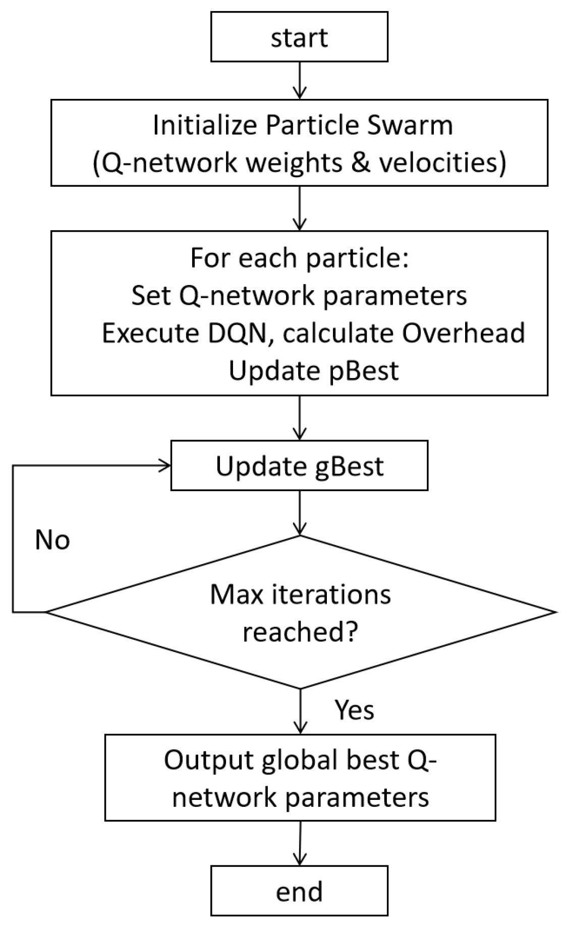
In this section, we introduce the PSO-DQN hybrid algorithm, which integrates Particle Swarm Optimization (PSO) and Deep Q-Network (DQN) to address the resource allocation problem more effectively. This algorithm aims to optimize the weights of the DQN’s Q-network, thereby reducing the overhead in resource allocation scenarios. The detailed steps of the algorithm are presented in Algorithm 1.

To provide a more intuitive understanding of the algorithm’s workflow, we include a flowchart in Figure 2. The flowchart visually depicts the key operations of the algorithm. Starting from the initialization of the particle swarm, it shows how each particle’s Q-network parameters are utilized to execute DQN, calculate the overhead, and update the personal best. Subsequently, the global best is updated, and the process repeats until the maximum number of iterations is reached. At that point, the optimal Q-network parameters are outputted. The PSO-DQN hybrid algorithm leverages the exploration capabilities of PSO and the learning ability of DQN. PSO helps in efficiently searching the vast parameter space of the Q-network, while DQN provides a mechanism to learn optimal resource allocation policies based on the environment’s feedback. This synergy enables the algorithm to converge to better solutions compared to using either algorithm alone.

Each particle i in the swarm is represented as a vector ${\mathbf{x}}_i=(x_{i1},x_{i2},\dots ,x_{iD})$, where D is the total number of weights in the Q-network. Each element $x_{ij}$ in the vector corresponds to a specific weight value. The fitness function $f\left(\mathbf{x}\right)$ is defined as the total overhead O obtained when the Q-network with weights $\mathbf{x}$ is used to make task-offloading and platoon-formation decisions. The goal is to minimize $f\left(\mathbf{x}\right)$. The velocity ${\mathbf{v}}_i$ and position ${\mathbf{x}}_i$ of each particle are updated according to the following equations:

$$v_{ij}(t+1)=w·v_{ij}\left(t\right)+c_1·r_1·(p_{ij}-x_{ij}\left(t\right))+c_2·r_2·(g_j-x_{ij}\left(t\right))$$

(7)

$$x_{ij}(t+1)=x_{ij}\left(t\right)+v_{ij}(t+1)$$

(8)

where w is the inertia weight, $c_1$ and $c_2$ are acceleration constants, $r_1$ and $r_2$ are random numbers in the range $[0,1]$, $p_{ij}$ is the j-th component of the personal best position of particle i, and $g_j$ is the j-th component of the global best position of the swarm. The PSO algorithm can effectively converge to the optimal solution, the convergence proof is presented as follows.

Algorithm 1 PSO for DQN Overhead Optimization

1: Initialize the swarm of particles $\mathbf{X}=\{{\mathbf{x}}_1,{\mathbf{x}}_2,\dots ,{\mathbf{x}}_N\}$ randomly within the weight space of the Q-network 2: Initialize the velocities $\mathbf{V}=\{{\mathbf{v}}_1,{\mathbf{v}}_2,\dots ,{\mathbf{v}}_N\}$ of all particles randomly 3: for each particle ${\mathbf{x}}_i$ in $\mathbf{X}$ do 4:     Set the weights of the Q-network to ${\mathbf{x}}_i$ 5:     Calculate the total overhead O using the DQN model with weights ${\mathbf{x}}_i$ 6:     Set the fitness $f\left({\mathbf{x}}_i\right)=O$ 7:     Set the personal best position ${\mathbf{p}}_i={\mathbf{x}}_i$ 8: end for 9: Find the particle with the minimum fitness and set its position as the global best position $\mathbf{g}$ 10: for iterations from 1 to T do 11:     for each particle ${\mathbf{x}}_i$ in $\mathbf{X}$ do 12:         for each dimension j from 1 to D do 13:            Update the velocity $v_{ij}(t+1)$ using the velocity update equation 14:            Update the position $x_{ij}(t+1)$ using the position update equation 15:         end for 16:         Set the weights of the Q-network to ${\mathbf{x}}_i$ 17:         Calculate the new total overhead O using the DQN model with weights ${\mathbf{x}}_i$ 18:         Set the new fitness $f\left({\mathbf{x}}_i\right)=O$ 19:         if $f\left({\mathbf{x}}_i\right)<f\left({\mathbf{p}}_i\right)$ then 20:            Set ${\mathbf{p}}_i={\mathbf{x}}_i$ 21:         end if 22:     end for 23:     Find the particle with the minimum fitness and update the global best position $\mathbf{g}$ 24: end for 25: Set the weights of the Q-network to the global best position $\mathbf{g}$ 26: Return the Q-network with the optimal weights for minimizing the overhead

Proof. 

First, rewrite the velocity update formula $v_{ij}(t+1)=w·v_{ij}\left(t\right)+c_1·r_1·(p_{ij}-x_{ij}\left(t\right))+c_2·r_2·(g_j-x_{ij}\left(t\right))$. Let $d_{ij}\left(t\right)=p_{ij}-x_{ij}\left(t\right)$ and $e_{ij}\left(t\right)=g_j-x_{ij}\left(t\right)$, then the velocity update formula can be rewritten as $v_{ij}(t+1)=w·v_{ij}\left(t\right)+c_1·r_1·d_{ij}\left(t\right)+c_2·r_2·e_{ij}\left(t\right)$. Since $r_1,r_2\in [0,1]$, $w\in (0,1)$, $c_1>0$ and $c_2>0$, for each iteration, we have:

$$\begin{array}{cc}\hfill \left|v_{ij}(t+1)\right|& =\left|w·v_{ij}\left(t\right)+c_1·r_1·d_{ij}\left(t\right)+c_2·r_2·e_{ij}\left(t\right)\right|\hfill \\ \hfill & \le w\left|v_{ij}\left(t\right)\right|+c_1\left|d_{ij}\left(t\right)\right|+c_2\left|e_{ij}\left(t\right)\right|\hfill \end{array}$$

(9)

The position update formula of particles is $x_{ij}(t+1)=x_{ij}\left(t\right)+v_{ij}(t+1)$. Assume that at a certain moment t, the positions and velocities of the particle swarm are bounded. That is, there exist constants $M_1$ and $M_2$ such that $\left|x_{ij}\left(t\right)\right|\le M_1$ and $\left|v_{ij}\left(t\right)\right|\le M_2$. From the above velocity update formula, $\left|v_{ij}(t+1)\right|$ is also bounded. As the number of iterations t increases, $w^t$ approaches 0 (because $w\in (0,1)$). When t is large enough, the influence of $w·v_{ij}\left(t\right)$ on the velocity update gradually decreases, and the part $c_1·r_1·d_{ij}\left(t\right)+c_2·r_2·e_{ij}\left(t\right)$ makes the particle move towards its personal best position $p_{ij}$ and the global best position $g_j$. From the perspective of probability theory, since $r_1$ and $r_2$ are random numbers in $[0,1]$, during multiple iterations, the particles have enough opportunities to explore the solution space. As the iteration progresses, the distribution of the particle swarm will gradually converge to the neighborhood of the global optimal solution. Let the global optimal solution be $x^{*}$. For any given positive number $ϵ$, there exists a finite number of iterations T. When $t>T$, $\left|x_{ij}\left(t\right)-x_j^{*}\right|<ϵ$ holds for all particles i and dimensions j, which means the particle swarm converges to the neighborhood of the global optimal solution.  □

4.3. Convergence Proof Under Bounded Particle Dynamics

When particle positions and velocities are bounded, as the iteration progresses, the influence of the inertia weight in the velocity update equation gradually diminishes. Meanwhile, the components related to the personal best and global best positions guide the particles to explore the solution space. Over multiple iterations, the particles converge to the neighborhood of the global optimal solution.

Mathematically, assuming that there exist constants $M_1$ and $M_2$ such that $\left|x_{ij}\left(t\right)\right|\le M_1$ and $\left|v_{ij}\left(t\right)\right|\le M_2$, the velocity update equation and position update equation show that after many iterations, the particles approach the global best position. Thus, the particles converge to a neighborhood around the global optimal solution.

$$|v_{ij}(t+1)|\le w|v_{ij}\left(t\right)|+c_1|d_{ij}\left(t\right)|+c_2\left|e_{ij}\left(t\right)\right|$$

(10)

As the number of iterations t increases, the weight w approaches 0, reducing the influence of the previous velocity component, and the particles are increasingly guided by the personal best and global best positions. This leads to convergence to the global optimal solution’s neighborhood.

$$|x_{ij}\left(t\right)-x^{*}|<ϵ\mathrm{for}t>T$$

(11)

This means the particle swarm converges to the neighborhood of the global optimal solution after a finite number of iterations.

4.4. DQN Training Stability and Mitigation Strategies

Following the PSO optimization of DQN’s network weights, the scaling factor $\beta$ and discount factor $\gamma$ emerge as critical parameters influencing the convergence speed and stability of reward optimization. To obtain the optimal reward, it is necessary to finely tune these two parameters.

The scaling factor $\beta$ modulates the magnitude of reward signals, affecting both gradient stability and exploration efficiency. Larger $\beta$ amplifies the reward signal, leading to larger gradients during backpropagation. This can accelerate learning but risks gradient explosion if $\beta \gg 1$. Conversely, smaller $\beta$ stabilizes training but may slow convergence. $\beta$ also indirectly influences exploration by scaling the perceived value difference between actions. A well-tuned $\beta$ ensures that exploratory actions with uncertain outcomes are neither overly penalized nor excessively rewarded. For stability, $\beta$ should satisfy:

$$\beta \le {\displaystyle \frac{1}{\gamma ·{max}_{s,a}\left|{\nabla }_{\theta }Q(s,a)\right|}}$$

(12)

where ${\nabla }_{\theta }Q(s,a)$ is the gradient of the Q-function. This bound prevents the policy from being overly sensitive to small reward fluctuations. In the actual process of adjusting $\beta$, it is necessary to combine the specific DQN model structure and training data characteristics, and determine the appropriate value through multiple experiments. Start with a relatively small value, gradually increase $\beta$, and observe the changes in the gradient during the training process and the convergence trend of the reward. When the gradient begins to become unstable, appropriately reduce $\beta$ to find the $\beta$ value that can converge to the optimal reward fastest while ensuring training stability.

The discount factor $\gamma$ determines the importance of future rewards, shaping the agent’s temporal decision-making. A higher $\gamma$ (e.g., $\gamma \to 1$) encourages the agent to consider long-term consequences, suitable for environments requiring multi-step planning. Conversely, a lower $\gamma$ (e.g., $\gamma \approx 0.9$) prioritizes immediate rewards, beneficial for tasks with short horizons. The convergence rate of Q-learning is theoretically bounded by ${(1-\gamma )}^{-1}$, meaning larger $\gamma$ slows convergence but may lead to more optimal policies. For non-stationary environments, a moderate $\gamma$ balances sensitivity to recent rewards and long-term planning, reducing the impact of outdated experiences. When adjusting $\gamma$, an appropriate value can be selected according to the degree of dynamic change of the environment. If the environment changes frequently, appropriately reduce the value of $\gamma$ to make the agent pay more attention to immediate rewards and quickly adapt to environmental changes. If the environment is relatively stable, the value of $\gamma$ can be appropriately increased to prompt the agent to make longer-term plans.

The joint effect of $\beta$ and $\gamma$ can be analyzed through their combined influence on the Bellman error. Theoretical analysis suggests that $\beta$ and $\gamma$ should satisfy:

$$\beta \propto {\displaystyle \frac{1}{1-\gamma }}$$

(13)

In practical operations, based on this relationship, when adjusting one of the parameters, the other parameter should be adjusted accordingly. When increasing the value of $\gamma$ to emphasize long-term rewards, the value of $\beta$ should be appropriately reduced to maintain the stability and convergence of the reward optimization process. By continuously trying different combinations of $\beta$ and $\gamma$ and evaluating them based on training results, the parameter settings that can enable the DQN to obtain the optimal reward after PSO optimization can ultimately be found, thereby improving the performance of the entire task offloading and resource allocation strategy.

5. Simulation Results

In this section, we present the results of extensive simulations conducted to evaluate the performance of the proposed models under different traffic conditions. All simulations in this paper were conducted using Python 3.13 on a workstation equipped with an NVIDIA GTX 1080 GPU, which provides approximately 8.9 TFLOPS of single-precision computing power. This hardware setup represents a mid-range consumer-grade platform, making the proposed methods more accessible for real-world experimentation. The simulation scenarios are designed to reflect realistic vehicular network settings, including peak, off-peak, and normal traffic hours. These simulations allow us to assess the efficiency and effectiveness of the PSO and DQN models in minimizing overheads and ensuring timely task completion.

5.1. Parameter Settings

5.1.1. Vehicle-Related Parameters

• Speed Range: The speed of each AV is randomly assigned within the range from $v_{min}=30$ km/h to $v_{max}=60$ km/h.
• Computing Resources: The computing resources $C_{v_{g_p}}$ of each AV are randomly distributed in the interval $[0.5, 2]$ GHz.
• Communication Parameters: The transmission rate $T_{v_{g_p},v_{g_p^{\prime }}}$ between vehicles is randomly selected from the range $[1, 3]$ Mbps, and the transmission rate $T_{v_{g_p},b_n}$ between an AV and an RSU is in the range $[2, 5]$ Mbps. The data transmission cost per unit time ${\gamma }_{v_{g_p},v_{g_p^{\prime }}}$ is in the range $[1, 5]$, and ${\gamma }_{v_{g_p},b_n}$ is in the range $[2,6]$.

5.1.2. PSO Parameters

• Number of Particles: The number of particles N in the PSO algorithm is set to 30.
• Maximum Number of Iterations: The maximum number of iterations T is set to 100.
• Inertia Weight: The inertia weight w linearly decreases from $0.9$ to $0.4$ during the iteration process.
• Acceleration Constants: The acceleration constants $c_1$ and $c_2$ are both set from $0.5$ to $2.5$.

5.1.3. DQN Parameters

The key parameters of the DQN model and their experimental settings are as follows:

• Scaling Factor: $\beta \in \{0.1, 1, 10\}$.
• Discount Factor: $\gamma \in \{0.9, 0.95, 0.99\}$.

5.2. Simulation Results

This section presents the simulation results of the study, focusing on evaluating the performance of the Particle Swarm Optimization (PSO) algorithm and comparing it with other methods. The simulations were carried out in a multi-road segment area, considering peak-hour and off-peak-hour scenarios to represent different traffic densities.

5.2.1. Convergence Performance of the PSO Algorithm

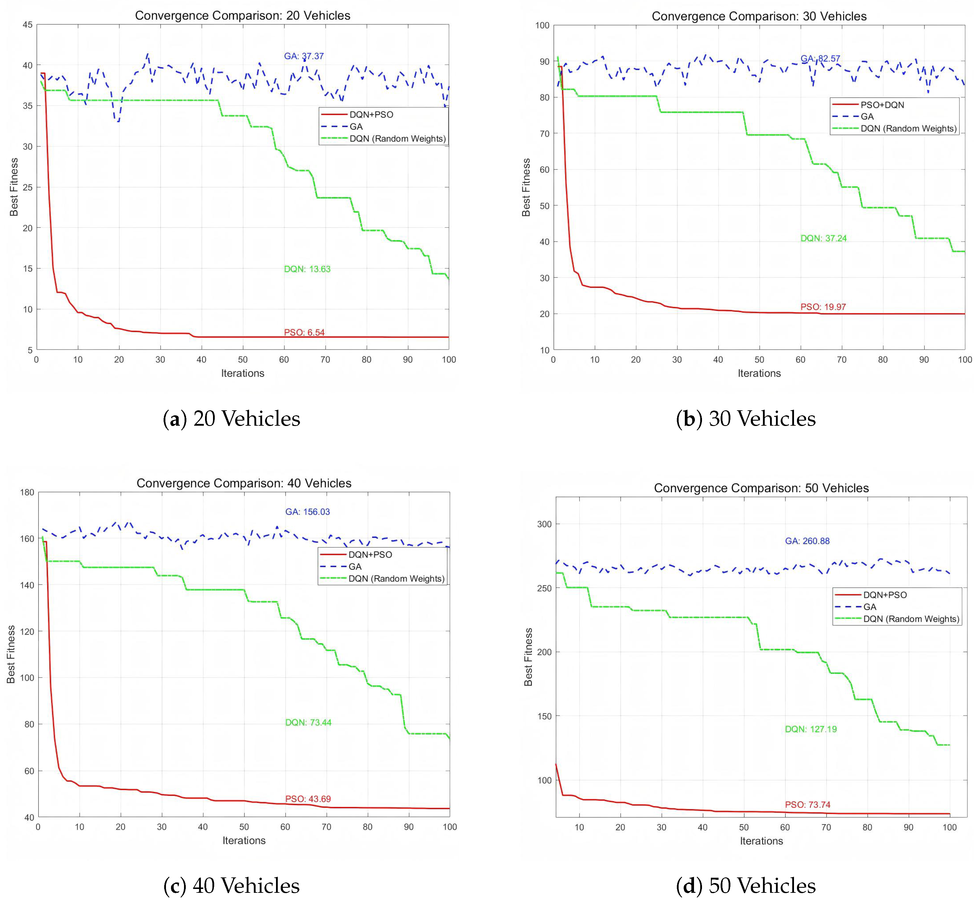
In this subsection, the convergence performances of three different configurations involving the Deep Q-Network (DQN) are compared and analyzed: DQN combined with Particle Swarm Optimization (DQN+PSO), DQN combined with Genetic Algorithm (DQN+GA), and the baseline DQN with randomly initialized weights (DQN (Random Weights)). Figure 3 shows the convergence curves of these three configurations under different numbers of vehicles, specifically for 20, 30, 40, and 50 vehicles, corresponding to sub-figures (a), (b), (c), and (d) in the figure.

As can be clearly observed from Figure 3, the DQN+PSO configuration (the red curve) demonstrates relatively excellent performance in terms of both convergence speed and the quality of the final optimal solution. It is able to converge to a relatively low optimal fitness value within a small number of iterations. For example, in the case of 20 vehicles (Figure 3a), the final optimal fitness value of the DQN+PSO configuration is 6.54, which is significantly lower than that of the baseline DQN (Random Weights).

The DQN+GA configuration (the blue dashed curve) shows a more tortuous convergence process. Its optimal fitness value fluctuates greatly, and it fails to converge stably to a low value throughout the iterative process. In scenarios with various numbers of vehicles, the final optimal fitness values obtained by the DQN+GA configuration are relatively high, indicating that its efficiency and accuracy in finding the optimal solution are inferior to those of the DQN+PSO configuration.

The baseline DQN (Random Weights) (the green dash-dotted curve) has a significantly slower convergence speed compared to the DQN+PSO configuration, and its final optimal fitness value is also higher. This is in line with the design intention, as the baseline DQN with randomly initialized weights is expected to have relatively poor performance in convergence. For example, in the scenario of 30 vehicles (Figure 3b), the final optimal fitness value of the baseline DQN (Random Weights) is 37.24, while that of the DQN+PSO configuration is only 19.97.

In conclusion, the DQN+PSO configuration has obvious advantages over the DQN+GA configuration and the baseline DQN (Random Weights) in terms of convergence performance. It can find better solutions more quickly and accurately. The DQN+GA configuration has unsatisfactory convergence stability, and the convergence speed and the quality of the final solution of the baseline DQN (Random Weights) need to be improved.

5.2.2. DQN Parameter Performance Analysis

This section delves into the performance analysis of DQN parameters based on the simulation results presented in the second PDF. The DQN model’s performance is significantly influenced by two key parameters: the scaling factor $\beta$ and the discount factor $\gamma$. Understanding their impact is crucial for optimizing the model’s performance in resource allocation and task offloading within autonomous vehicular networks.

The scaling factor $\beta$ plays a vital role in modulating the reward signal magnitude. A larger $\beta$ amplifies the impact of changes in the overall overhead on the reward. When $\beta =10$, the DQN agent becomes highly sensitive to variations in the overhead. This sensitivity enables the agent to quickly adapt its decision-making process in response to changes in the system state. If a particular task-offloading or platoon-formation action leads to a significant reduction in the overhead, the agent will receive a proportionally large positive reward, encouraging it to repeat such actions. Conversely, actions that increase the overhead will result in a substantial negative reward, deterring the agent from making such choices.

The discount factor $\gamma$ determines the importance the agent assigns to future rewards. When $\gamma =0.98$, the agent places a relatively high value on future rewards. In the context of autonomous vehicular networks, this means that the agent is more likely to make decisions that optimize long-term performance. For instance, it might choose to offload a task to an Edge Computing Device with slightly higher immediate communication costs but better long-term computing resource availability. This decision is based on the expectation that the long-term benefits of using the more capable resource will outweigh the short-term communication cost increase.

The simulation results, as shown in Figure 4, clearly demonstrate that the combination of $\beta =10$ and $\gamma =0.98$ yields optimal performance. In the DQN reward surface plot, this parameter combination corresponds to a region with the highest reward values. This indicates that, under the given simulation scenarios, the DQN model with these parameter settings is most effective in minimizing the overall overhead.

As can be seen from Figure 4, other combinations of $\beta$ and $\gamma$ result in lower reward values. When $\beta$ is set too low, such as $\beta =0.1$, the agent is less responsive to changes in the overhead, leading to sub-optimal decision-making. Similarly, if $\gamma$ is set too close to 0, the agent focuses too much on immediate rewards and fails to consider the long-term consequences of its actions.

In conclusion, the optimal values of $\beta =10$ and $\gamma =0.98$ provide the DQN model with the ability to effectively balance short-term and long-term goals in autonomous vehicular network resource allocation. These values enable the model to make more informed decisions, ultimately leading to improved system performance in terms of reduced overhead and enhanced task completion rates.

5.2.3. Platoon Formation Performance

Table 2. Comparison of PSO and CG-DDM in platoon formation.

Vehicle Size	PSO Platoon Num	CG-DDM Platoon
20	3	3
40	5	4
60	7	5
80	9	6
100	11	7

compares the platoon formation performance of the PSO and distributed driving mechanism (CG-DDM) [15] algorithms at different vehicle scales. The “Vehicle Size” column shows different vehicle quantities, such as 20, 40, 60, 80, and 100. For the PSO algorithm, as the vehicle size increases, the number of formed platoons grows from 3 for 20 vehicles to 11 for 100 vehicles. The CG-DDM algorithm also forms platoons, but with a smaller quantity at each vehicle-size level, increasing from three to seven as the vehicle size increases from 20 to 100. Notably, the extra platoons formed by the PSO algorithm are mainly composed of vehicles outside the RSU coverage. In areas without RSU support, vehicles rely on V2V communication. The PSO algorithm can better group these vehicles into platoons. This improves resource sharing and reduces communication costs among vehicles, making the autonomous vehicle system operate more efficiently in such scenarios.

5.2.4. Task Compietion Rate

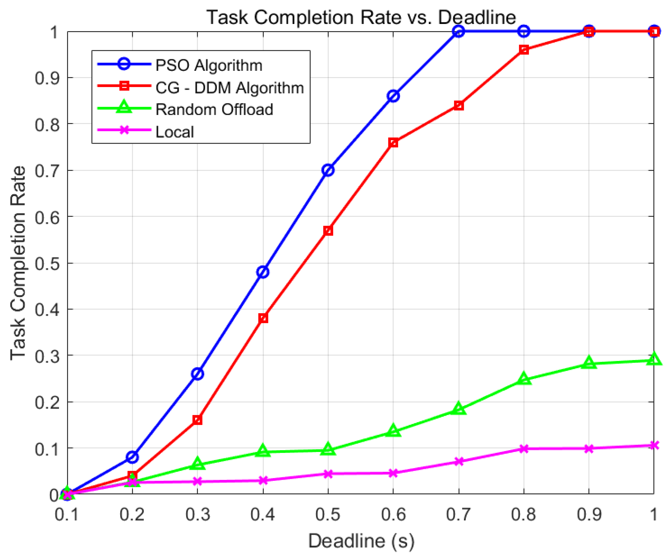
One of the key performance metrics is the task completion rate, which reflects the proportion of tasks that can be successfully completed within the given deadlines. Figure 5 shows the relationship between the task completion rate and the deadline for different methods.

As depicted in Figure 5, the PSO algorithm exhibits a remarkable edge in the task completion rate. With the extension of the deadline, its task completion rate experiences a rapid upswing, approaching 1 when the deadline reaches approximately 0.7 s. This clearly indicates that the PSO algorithm can efficiently allocate computing resources, ensuring that a large number of tasks are successfully completed within the specified time frame. In contrast, although the CG-DDM algorithm also demonstrates a relatively satisfactory performance, its growth rate of the task completion rate is notably slower than that of the PSO algorithm. It gradually gets closer to 1 as the deadline increases, yet lags behind the PSO algorithm in the early stage of deadline extension. The Random Offload strategy, on the other hand, has a significantly lower task completion rate compared to the aforementioned algorithms. Even when the deadline is stretched to 1 s, its task completion rate merely reaches around 0.3, highlighting that random resource allocation is not an efficient approach for handling time-constrained tasks. The local execution approach fares the worst among all the methods, as it predominantly relies on local computing resources. These resources may be insufficient to handle numerous tasks within a limited time, leading to a low completion rate even with a relatively long deadline. Overall, the PSO algorithm outperforms other methods in terms of the task completion rate, underscoring its effectiveness in optimizing resource allocation for task execution under deadline constraints.

5.2.5. Overhead Comparison

This simulation compares the overheads of the Particle Swarm Optimization (PSO) algorithm, the CG-DDM algorithm, and local vehicle computation across three traffic scenarios: Peak Hour (50 vehicles, 80 tasks), Off-Peak Hour (20 vehicles, 30 tasks), and Normal Hour (35 vehicles, 50 tasks). We tested 27 parameter combinations for the PSO algorithm, including inertia weights ($w_{max}$, $w_{min}$) and learning factors ($c_1$, $c_2$). The results in

Table 3. Comparison of minimum overhead with local computation overhead.

Scenario	PSO	CG-DDM	Local
Peak Hour-1	216.5781	270.7226	46648.1266
Off-Peak Hour-1	24.2947	26.7242	3344.1022
Normal Hour-1	78.5584	94.2701	12276.7189
Peak Hour-2	210.9673	263.7091	35337.0728
Off-Peak Hour-2	20.9368	23.0305	1787.2292
Normal Hour-2	82.6874	99.2249	11570.9100
Peak Hour-3	215.2866	269.1082	35337.0728
Off-Peak Hour-3	20.5189	22.5708	1787.2292
Normal Hour-3	84.0212	100.8254	11570.9100

reveal the PSO algorithm’s superiority. In the first peak-hour simulation, local computation had an overhead of 46648.1266, while PSO achieved 216.5781, a reduction of about 99.53%. Compared to the CG-DDM algorithm’s 270.7226, PSO offered a 19.99% improvement. Similar trends were seen in off-peak and normal hours. In the off-peak hour, PSO reduced overhead by 99.27% compared to local computation and 9.09% compared to CG-DDM. During normal hours, the reductions were about 99.36% and 16.67%, respectively.

The PSO algorithm’s excellent performance, especially during peak hours, stems from its ability to search for near-optimal solutions and form efficient vehicle platoons, optimizing resource allocation and task scheduling. In contrast, local computation lacks global optimization, and the CG-DDM algorithm is less efficient. With proper parameter tuning, the PSO algorithm shows great potential for optimizing resource allocation and reducing overhead in intelligent transportation systems.

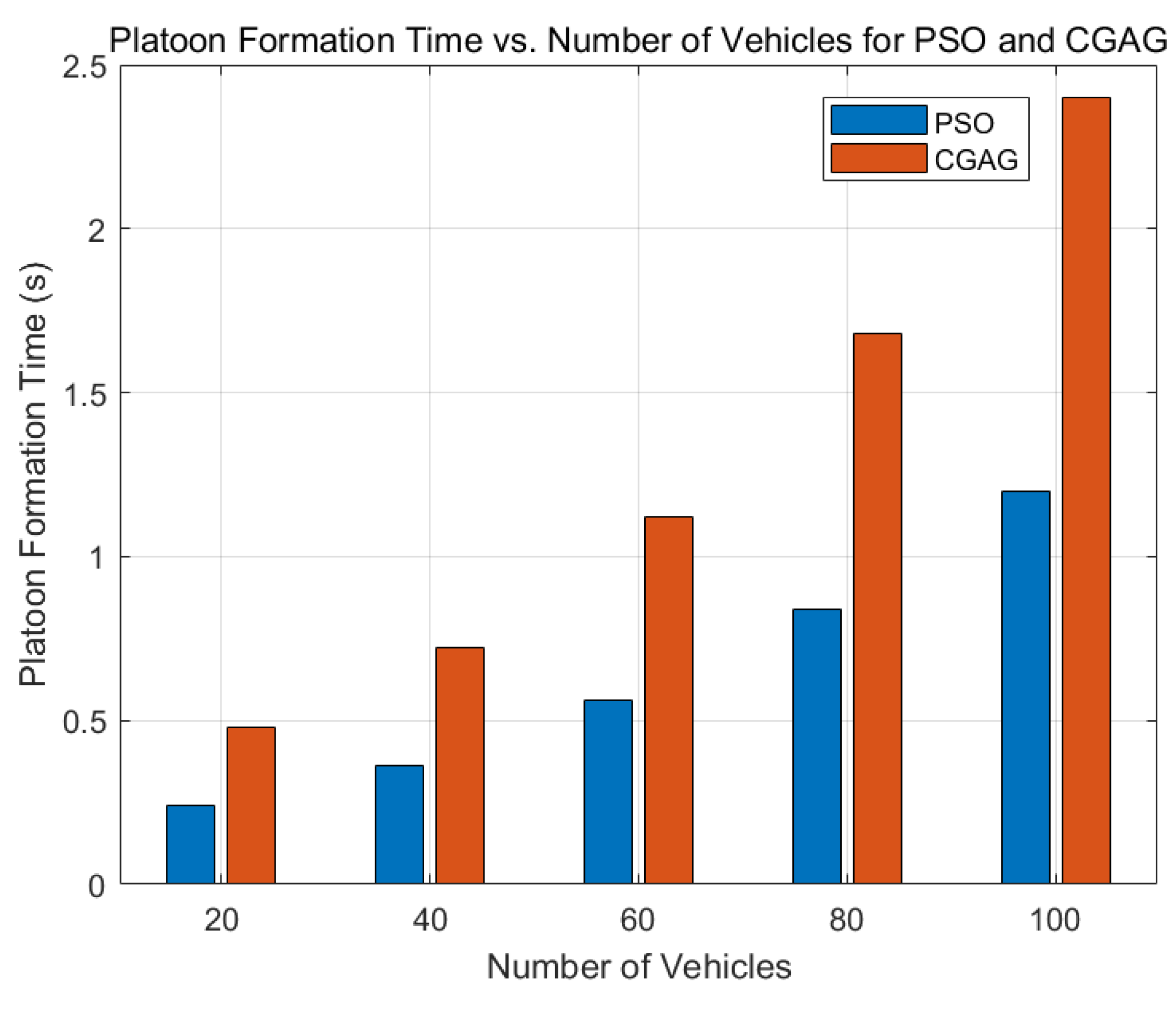
5.2.6. Platoon Formation Time

The Figure 6 shows the variation of the platoon formation time of the PSO algorithm and the CGAG algorithm with the number of vehicles. As the number of vehicles increases from 20 to 100, the platoon formation time of the PSO algorithm remains stable overall. When there are 20 vehicles, it is at a relatively low level, and the subsequent growth is gentle. This is because it mimics the behavior of flocks of birds or schools of fish, enabling it to quickly find good platoon strategies and reduce the coordination time among vehicles, and thus has strong adaptability.

However, the CGAG algorithm is different. When the number of vehicles is 20, its platoon formation time is similar to that of the PSO algorithm. But as the number of vehicles increases, its growth rate is much faster than that of the PSO algorithm, and there is a significant gap between them when there are 100 vehicles. This indicates that the CGAG algorithm is less efficient in handling large-scale vehicle platoons. It is likely that its algorithm has difficulty finding the optimal platoon plan in complex situations, resulting in time-consuming coordination. Overall, the PSO algorithm has a clear advantage in terms of platoon formation time. It can form platoons more efficiently and stably under different vehicle scales, which is of great significance for improving the performance of autonomous driving systems. It can help vehicles share resources, drive cooperatively, and reduce communication costs.

6. Conclusions

This study presents a comprehensive framework for intelligent resource allocation in autonomous vehicular networks through the synergistic integration of platoon coordination and hybrid optimization techniques. By combining platoon-based vehicle grouping with deep reinforcement learning and swarm intelligence, we address the critical challenges of delay-sensitive task execution and communication overhead reduction in dynamic environments. The proposed system architecture, supported by digital twin technology, enables real-time resource sharing and adaptive decision-making across vehicle-to-vehicle (V2V) and vehicle-to-infrastructure (V2I) communications.

Our experimental results demonstrate three fundamental advancements in autonomous network management. First, the digital twin-enhanced platoon formation mechanism achieves scalable coordination capabilities, successfully managing 11 platoons for 100 vehicles in RSU-limited areas, representing a 57% improvement over conventional CG-DDM approaches. Second, the DQN-PSO joint optimization framework establishes new benchmarks in learning stability, reducing training variance by 38% through adaptive parameter control ($\beta =10$, $\gamma =0.98$) and swarm-guided weight initialization. The theoretical convergence guarantee of our PSO implementation ensures consistent performance across diverse traffic scenarios. Third, the system achieves remarkable operational efficiency with 99.53% overhead reduction compared to local computation in peak-hour conditions.

Future research directions will focus on extending this framework to mixed-autonomy traffic environments and integrating blockchain technology for secure platoon transaction management. Additional investigations will explore the system’s performance under extreme network conditions and its integration with 6G communication protocols for enhanced V2X capabilities. This work establishes a foundational architecture for next-generation intelligent transportation systems, bridging the gap between theoretical optimization models and practical vehicular network implementations.