Joint Sparse Estimation Method for Array Calibration Based on Fast Iterative Shrinkage-Thresholding Algorithm

Abstract

Existing array calibration methods rely on the geometric characteristics of the array or signal matrix, which limits their flexibility and robustness. This study addresses this challenge by proposing a novel joint sparse estimation method for array gain and phase calibration. By leveraging the sparsity of calibration signals and the dictionary mismatch model, the proposed method, based on the fast iterative shrinkage-thresholding algorithm (FISTA), jointly estimates the discrete on-grid azimuths and continuous off-grid offsets of the direction of arrival (DOA) of calibration signals. The method employs a spatial domain filtering technique based on the maximum a posteriori probability to mitigate the bias induced by phase errors in the calibration signal estimation, enhancing calibration accuracy. Furthermore, the iterative estimation framework was optimized to extend the applicability of the method from linear to uniform planar arrays. The results demonstrated that the root mean squared error (RMSE) of the beam pattern for various array types decreased by one to two orders of magnitude after calibration. Compared with existing state-of-the-art methods, the proposed approach exhibited stable performance and superior estimation accuracy under conventional signal-to-noise ratio conditions. Moreover, the proposed method maintained high stability and lower RMSE as the gain and phase error values increased.

1. Introduction

In the signal processing of phased array systems, the gain and phase response characteristics of each array element and its conditioning circuit are assumed to be consistent. However, owing to limitations in array processing technology, performance biases in conditioning circuits, ambient temperature variations, multichannel mutual coupling, device aging, and other factors, the response characteristics of array elements deviate from the ideal in practical scenarios, resulting in gain and phase errors in the transmitted signals [1,2]. These errors result in energy leakage in the main lobe of the array beam pattern, reduced peak value, increased side lobe intensity, and degraded resolution due to beam fusion when imaging adjacent targets. Array calibration methods that estimate and correct the gain and phase errors of an array have been proposed to address these issues by comparing the expected logical response signals with the actual measured response signals of the array. Array calibration methods can be categorized into two main types: active calibration, which utilizes known and accurate calibration signals, and autocalibration, which employs unknown calibration signals [3,4].

The active calibration method considers the calibration signal orientation as known information; that is, an accurate, ideal array signal response is available, enabling the array gain and phase error to be directly estimated. In [5], several calibration sources were placed at precise positions, successively transmitting calibrated signals; equations were constructed based on the planar array response. These equations were then used to solve for the gain and phase errors in the array response characteristics. In addition, algorithms such as maximum likelihood estimation [6] and the least squares method [7] have been extensively applied to address array error calibration and have achieved promising results. However, although the active calibration method has high error estimation accuracy owing to its known accurate signal orientation, obtaining a precise orientation of the calibration signal in practice is challenging, which limits the application scenarios of the active calibration method.

In the autocalibration method, the azimuth of the calibration signal is unknown, and the calibration signal and array errors are estimated simultaneously. This method is more commonly used in real-world scenarios and has thus been widely studied. Owing to the coupling of the array error and calibration source position, studies typically estimate the direction of arrival (DOA) of the calibration source first and then use spatial filtering to calibrate the gain and phase errors of the array. DOA estimation algorithms include multiple signal classification (MUSIC) [8], estimation of signal parameters via rotation invariance techniques [9], a three-step iterative (TSI) algorithm [10,11], phase interferometry DOA estimation [12,13,14,15], compressed sensing (CS) methods such as Bayesian compressed sensing (BCS) and convex optimization (CVX) [16,17,18,19], and deep learning methods [20,21,22,23]. The symmetric property of the uniform array manifold and covariance matrices, both of which are Toeplitz matrices [24,25,26], is utilized to resolve the phase ambiguity problem in uniform arrays. Recently, super-resolution algorithms such as deconvolution beamforming have significantly improved the beam resolution via CLEAN methods [27,28], Richardson–Lucy methods [29,30,31], BCS [32,33], and fast iterative shrinkage-thresholding algorithm (FISTA) [34,35,36]. Among them, the FISTA based on the gradient algorithm has been widely used and studied in the field of signal and image processing owing to its excellent convergence speed, stability, and optimization performance [37,38,39]. However, such studies have limitations in terms of the off-grid estimation, signal-to-noise ratio (SNR), array configuration, array gain, and phase error.

Some characteristic structure- and Toeplitz property-based methods mostly rely on the array geometric characteristics or prior information related to the array structure. These methods have good performance in the corresponding array types but lack versatility for multi-array types. Spectral peak search, signal subspace, CS, and other signal spatial domain information-based methods reduce the array configuration requirements for calibration. However, these methods improve DOA accuracy by increasing the grid density of the preset calibration signal direction, and their computational complexity can reach the third or fourth power of the product of the number of grid points and the number of array elements, resulting in significant calculation delays in large-scale arrays or high-precision scenarios.

Moreover, existing autocalibration methods still face challenges in terms of general applicability and robustness against noise. Hence, developing an array calibration method that is independent of the array geometry and has strong noise resistance is of considerable significance. Therefore, this study proposes a joint sparse estimation method for array calibration using FISTA. This method is based on the sparse signal dictionary mismatch model and jointly estimates the discrete grid points and continuous offsets of the sparse calibration signal direction, as well as the signal and beam domain DOA, which enhances the degrees of freedom estimation of the calibration signal while avoiding the sharp increase in computational load caused by refining the estimation grid points. The method leverages calibration models and a joint estimation framework that is not restricted by array shape, thereby improving the universality of the calibration method. In addition, it employs maximum a posteriori spatial filtering to correct phase error interference in the calibration signal direction estimation, thereby effectively optimizing the calibration accuracy of amplitude and phase errors.

The remainder of this paper is organized as follows: Section 2 introduces and analyzes the joint sparse estimation method for array calibration based on FISTA. In Section 3, a planar array is used to evaluate the efficiency of the proposed method. Section 4 discusses the experimental results.

2. Materials and Methods

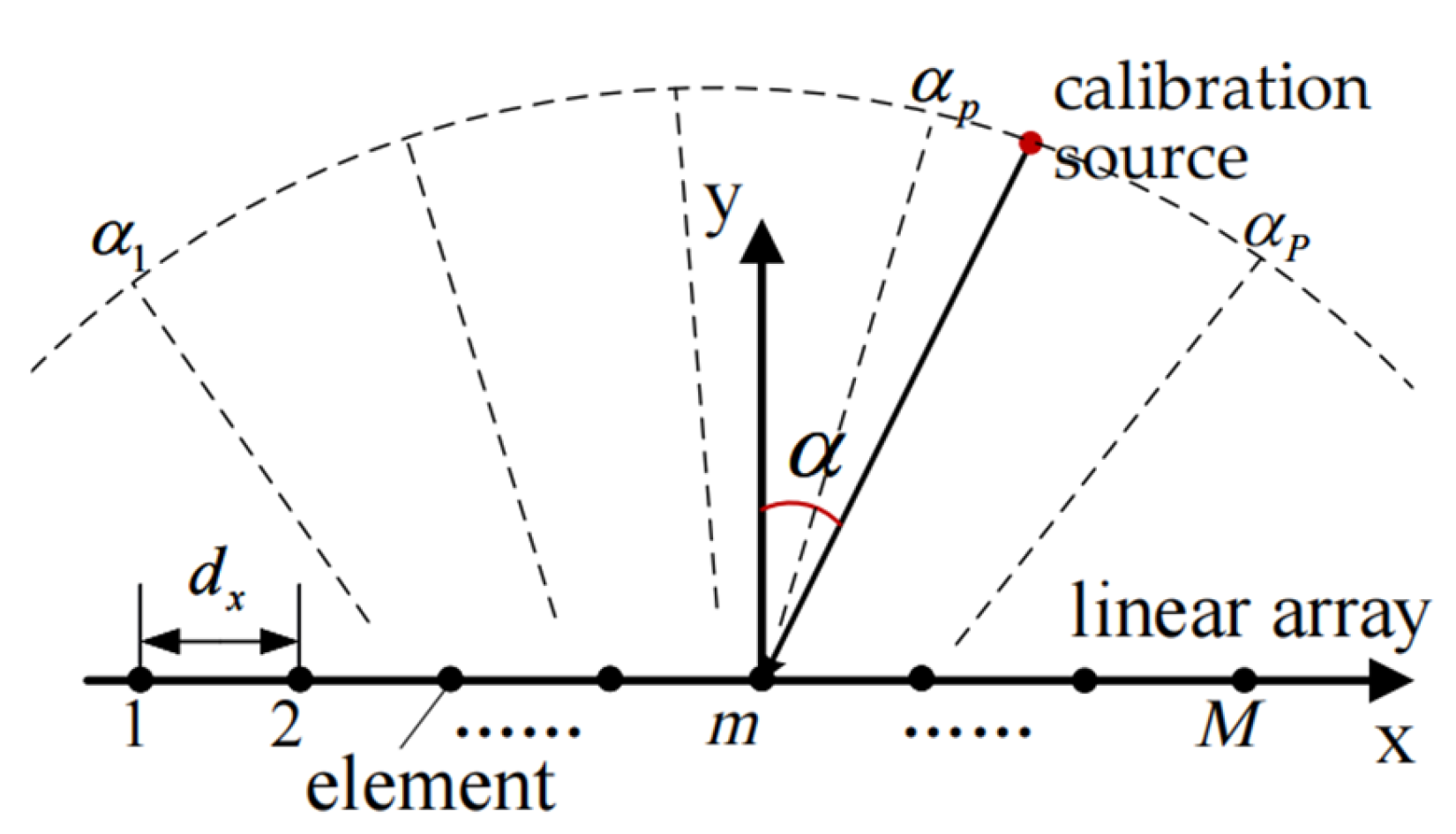
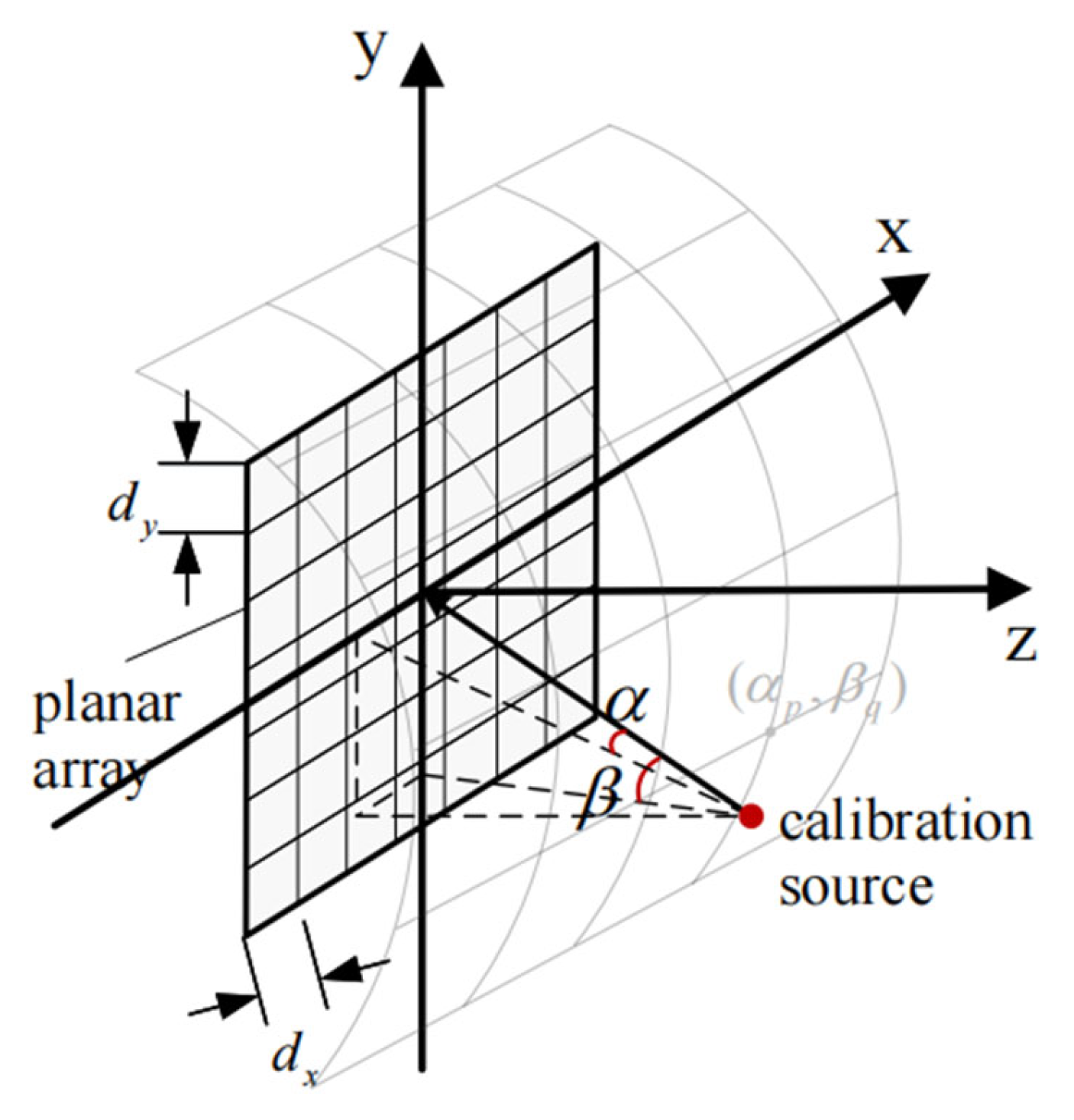
2.1. Array Calibration Signal Model

A uniform linear array with M elements is centered at the origin of the coordinate system (Figure 1). Let the element spacing of the array be d_x and the coordinates of the mth element be denoted as d_x(m) = (m − M + 1/2)d_x. In the far-field region, the ideal response signal at array element m for the incident signal from angle α is

$$x(m)=p{e}^{j\varphi }\times e^{j2\pi d_x(m)\sin \alpha /c}+{\epsilon }_m$$

(1)

where p represents the signal strength value, φ is the initial phase offset of the time-domain signal emitted by the calibration source, f denotes the signal frequency, c is the propagation speed of the signal in the current medium, and ε_m is the noise that is independently and identically distributed. Since array errors are mainly caused by factors such as machining accuracy, resistance and capacitance errors, environmental temperature, and humidity, the total error is caused by the superposition of multiple random errors. Therefore, selecting Gaussian noise with a normal distribution can simply and effectively simulate real noise.

Suppose there are phase and gain errors in the array. The gain error of element m is denoted as ξ_m and the phase error is τ_m. The actual response of the element m is expressed as follows:

$$\widehat{x}(m)=s\times {\xi }_m{e}^{j[2\pi f{d}_x(m)\sin \alpha /c+{\tau }_m]}+{\epsilon }_m$$

(2)

where s = pejφ. Here, the gain error ξm follows a Gaussian distribution with a mean of 1; the phase error τ_m follows a zero-mean Gaussian distribution.

In contrast to linear arrays, planar arrays provide beam resolution in both horizontal and vertical dimensions. First, a uniform planar array is used as an example to illustrate the angle estimation method for multidirectional calibration signals. The uniform planar array contains M × N receiving elements (Figure 2). The azimuth and elevation angles are denoted as α and β, respectively, with P representing horizontal beams and Q representing vertical beams. The signal from the (α_p, β_q) direction is the response of the (m, n) element of the planar array to the incident calibration signal and can be expressed as follows:

$$\begin{array}{ll}x(m,n)& ={\displaystyle {\sum }_{p=1}^P{\displaystyle {\sum }_{q=1}^Q{s}_{pq}}}\times e^{j2\pi [d_x(m)\sin {\alpha }_p+d_y(n)\sin {\beta }_q]/c}+{\epsilon }_{mn}\\ & ={\displaystyle {\sum }_{p=1}^P{\displaystyle {\sum }_{q=1}^Q{s}_{pq}}}\times a(m,n,p,q)+{\epsilon }_{mn}\end{array}$$

(3)

where d_x(m) = (m − (M + 1)/2)d_x and d_y(n) = (n − (N + 1)/2)d_y.

The two-dimensional array response is compressed into a vector x ∈ C^MN, and the four-dimensional sensing matrix is compressed into a two-dimensional matrix A ∈ C^MN×PQ to facilitate matrix computation. The matrix computation form is x = As + ε.

In the element response of the planar array, the signal components in the horizontal and vertical directions are coupled multiplicatively. Jointly estimating the on-grid indices and off-grid offsets in both directions involves third-order conic mapping, which increases computational complexity by an order of magnitude compared with single-direction estimation. Let Λ = MNPQ; then, the computational complexity of a single iteration is O(Λ² log(Λ)), where A_mn,pq is the element at the (mN + n)th row and (pQ + q)th column of A.

2.2. Joint Sparse Estimation of DOA

Considering the linear array first, the precise position of the calibration source or target is unknown in the autocalibration scenario involving array gain and phase errors. Hence, accurate incident signal information has to be obtained through DOA estimation to construct the ideal array response; then, this has to be combined with the actual array response to estimate the gain and phase errors of each array element.

When the distribution of the target signal is unknown, the continuous signal angle distribution is approximated by dividing the array observation domain into P uniform or nonuniform grid points, with each grid point corresponding to a candidate incident signal angle. The array response is given by

$$\begin{array}{ll}x(m)& ={\displaystyle {\sum }_{p=1}^P{s}_p\times e^{j2\pi f{d}_x(m)\sin \alpha /c}+{\epsilon }_m}\\ & ={\displaystyle {\sum }_{p=1}^P{s}_p\times a(m,p)+{\epsilon }_m}\end{array}$$

(4)

This equation can be expressed in matrix form as x = As + ε, where the array response vector x ∈C^M, and the observation matrix A∈ C^M×P. Let A_mp = a(m, p), and the signal vector s ∈ C^P. In practical applications, L ≪ P; hence, the signal vector s is typically regarded as a sparse vector.

Owing to matrix size limitations and computational load, the grid intervals of the candidate signal directions are typically not densely spaced. In this case, the actual incident angle of the target signal is unlikely to coincide with discrete grid points, and estimation errors are inevitable. This study addresses this issue by introducing a continuous correction term to optimize the off-grid model, enabling it to estimate off-grid incident signals.

$$\begin{array}{l}x=(A+E\mathit{\Delta })s+\epsilon \\ \Delta =\mathrm{diag}(\widehat{\alpha })\\ \widehat{\alpha }={[{\alpha }_1^{\prime }-{\alpha }_1,{\alpha }_2^{\prime }-{\alpha }_2,\dots ,{\alpha }_P^{\prime }-{\alpha }_P]}^T\end{array}$$

(5)

where ${\widehat{\alpha }}_p$ denotes the difference between the actual incident signal angle α_p′ closest to the grid point p and the angle α_p at the grid point; that is, the off-grid angle offset. E represents the off-grid correction term of the observation matrix. In this method, E is set as the first-order Taylor expansion of the observation matrix, and its derivation is as follows:

$$E_{mp}={\displaystyle \frac{\partial A_{mp}}{\partial \alpha }}=-j2\pi f{d}_x(m)\cos {\alpha }_p/c\times a(m,p)$$

(6)

According to the definition in $\widehat{\alpha }$$()$, the off-grid angle offset should not exceed half the grid angle spacing to avoid index confusion caused by out-of-bound offsets. If the grid points are uniform and the corresponding spacing is 2D_α, the constraint can be expressed as

$$\forall \left|{\widehat{\alpha }}_p\right|=D_{\alpha }$$

(7)

Let d = $\hat{\mathit{\alpha }}$ ⊙ s. Based on the LASSO theory, the DOA estimation problem of the off-grid model can be expressed as

$$\begin{array}{c}\min {\displaystyle \frac{1}{2}}{‖As+Ed-x‖}_2^2+\lambda {‖s‖}_{2,1}\\ s.t.\left|d\right|\le D_{\theta }\times s\end{array}$$

(8)

where λ||s||_2,1 is a penalty function term for ensuring sparsity, and it is defined as

$${‖s‖}_{2,1}={\displaystyle {\sum }_{p=1}^P\sqrt{s_p^2}}$$

(9)

Combining the ℓ₁ and ℓ₂ norms in the penalty function term can better constrain the complex incident signals with non-zero initial phases.

From the above definition and derivation, a non-zero value is meaningful only when the corresponding incident signal s_i is also non-zero for any element d_i in d. By leveraging this correlation, a joint sparse estimation of s and d is performed, rather than an alternating iterative solution. Let Φ = [A, E] ∈ C^M×2P and u = [s^T, d]^T ∈ C^2P, then Equation (8) can be rewritten as

$$\begin{array}{c}\min {\displaystyle \frac{1}{2}}{‖\mathbf{\Phi }u-x‖}_2^2+\lambda {‖u‖}_{2,1}\\ s.t.\left|d\right|\le D_{\theta }\times s\end{array}$$

(10)

The sparse penalty function term of the joint estimation item u is modified as follows:

$${‖u‖}_{2,1}={\displaystyle {\sum }_{p=1}^P\sqrt{u_p^2+u_{p+P}^2}}$$

(11)

Based on the joint sparsity of u, Equation (10) is treated as a sparse linear inverse problem, which can be solved using a linear inverse problem method optimized explicitly for this purpose. In this study, based on the traditional FISTA method and considering the joint sparsity of the model, the gradient calculation is improved using the Moreau envelope. The fixed step size is optimized to match the dynamic gradient descent step size obtained through a line search, thereby accelerating the convergence of the iteration.

Let $f(u)=1/2{‖\mathbf{\Phi }u-x‖}_2^2+\lambda {‖u‖}_{2,1}$, $g(u)=1/2{‖\mathbf{\Phi }u-x‖}_2^2$, and $h(u)=\lambda {‖u‖}_{2,1}$. The complex gradient of g(u) can be derived as

$$\nabla g(u)={\mathbf{\Phi }}^H(\mathbf{\Phi }u-x)$$

(12)

h(u) is a set of discrete points and is discontinuous, as noted in [40]; hence, the gradient of its continuous and differentiable Moreau envelope function is adopted as a substitute for the gradient. The Moreau envelope function with parameter η is given by

$$h_{\eta }(u)=\min \{h(v)+{\displaystyle \frac{1}{2\eta }}{‖v-u‖}_2^2\}$$

(13)

The gradient of the Moreau lower envelope function h_µ(u) can be expressed as

$$▽h_{\eta }(u)={\displaystyle \frac{1}{\eta }}(u-P_{h_{\eta }}(u))$$

(14)

Let P_hη(·) denote the mapping of the function h_η(·), and λ is set as the threshold. The gradient mapping corresponding to the lower envelope function is as follows:

$$\begin{array}{c}{P}_{h_{\eta }}(u_p)={\displaystyle \frac{s_p}{\sqrt{s_p^2+d_p^2}}}\max (\sqrt{s_p^2+d_p^2}-\lambda ,0)\\ P_{h_{\eta }}(u_{p+P})={\displaystyle \frac{d_p}{\sqrt{s_p^2+d_p^2}}}\max (\sqrt{s_p^2+d_p^2}-\lambda ,0)\end{array}$$

(15)

The gradient of the objective function f(u) in Equation (10) is derived as follows:

$$\begin{array}{ll}▽f(u)& =▽g(u)+▽h_{\eta }(u)\\ & ={\mathbf{\Phi }}^H(\mathbf{\Phi }u-x)+[u-P_{h_{\eta }}(u)]\end{array}$$

(16)

In the conventional FISTA method, after determining the function gradient, a fixed step size is used for gradient descent and nonlinear soft thresholding. The formula for the kth iteration is as follows:

$$u^{(k)}=P+(y^{(k)}+\mu ▽f(y^{(k)}))$$

(17)

The gradient descent step size µ is typically the reciprocal of the Lipschitz constant of the observation matrix. In this joint estimation problem, the fixed gradient step size is set to $\mu =1/({‖\mathbf{\Phi }u‖}_2^2+1/\lambda )$. A fixed gradient descent step size simplifies computation by eliminating the need to update the step size at each iteration. However, this may lead to slower convergence and an increased risk of becoming trapped in local optima.

The proposed joint estimation method addresses the issue of slow convergence with fixed step sizes by adopting a line search to dynamically select the gradient descent step size for each iteration, thereby avoiding overly small steps and accelerating convergence. This method is based on the Wolfe conditions in the optimization process. The gradient step size is calculated through a binary search. The Wolfe conditions include the following constraints:

$$\begin{gathered} f(u^{(k)}+{\mu }^{(k)}{c}^{(k)})\le f(u^{(k)})+c_1{\mu }^{(k)}▽f^T{u}^{(k)}{c}^{(k)} \\ ▽f^T(u^{(k)}+{\mu }^{(k)}{c}^{(k)})c_2▽f^T(u^{(k)})c^{(k)} \end{gathered}$$

(18)

where c^(k) is the gradient descent direction vector and c₁ and c₂ are the hyperparameters of the Wolfe conditions, typically set as 0 < c₁ < c₂ < 1. Equation (18) is the Armijo sufficient descent condition, which ensures that the objective function f(u^(k)) decreases monotonically. Evidently, when c₁ takes a smaller value, a smaller gradient descent step size μ^(k) can satisfy the Armijo sufficient descent condition, effectively preventing the step size from being too large and skipping the optimal point. However, this condition does not guarantee a global optimum, and there is a risk of getting trapped in a local minimum. Moreover, an excessively small step size may result in slow convergence. In addition, a curvature condition in the Wolfe criterion is introduced to ensure that the function decreases sufficiently along the gradient descent direction, thereby avoiding a step size that is too small.

The combination of both Wolfe conditions ensures that the step size is neither too large nor too small while maintaining sufficient descent along the gradient direction. This renders the selection of the gradient step size at each iteration more reasonable and effectively accelerates convergence. The bisection search method is adopted to determine the gradient step size µ^(k) that satisfies the constraints for the current iteration. Let r^(k) be the intermediate vector after gradient descent; then, the update formula for gradient descent with a dynamic step size can be rewritten as

$$r^{(k)}=y^{(k)}+{\mu }^{(k)}▽f(y^{(k)})$$

(19)

After completing the gradient descent calculation, nonlinear mapping is applied to the intermediate result r^(k) to obtain the current iteration result u^(k). Considering the joint estimation characteristics, the proposed FISTA-based algorithm optimizes conventional non-negative mapping by transforming it into a mapping process based on a two-dimensional convex cone projection. For the pth joint estimation pair [r_p, r_{p + P}] in r^(k), the mapping calculation is derived as

$$P(r_i)=P(\left|[r_p,r_{p+P}]\right|)=\left\{\begin{array}{ll}[r_p,r_{p+P}],& \left|r_{p+P}\right|\le -D{r}_p\\ [0,0],& r_p/D\le r_{p+P}\le -r_p/D\\ \kappa [r_p,r_{p+P}],& r_{p+P}\ge D{r}_p,r_{p+P}\ge -r_p/D\\ -\kappa [r_p,r_{p+P}],& r_{p+P}\le -D{r}_p,r_{p+P}\le r_p/D\end{array}\right.$$

(20)

where $\kappa ={\displaystyle \frac{r_p+\left|D\times r_{p+P}\right|}{1+D^2}}$. The above mapping operation is used to implement the requirement in Equation (10) that the angle offset $\widehat{\mathit{\alpha }}$ must not exceed the allowed angular range.

The joint estimation that deviates from the constrained region after the gradient descent calculation is projected back using the midpoint constraint of the grid points.

The subsequent step size update and Nesterov acceleration are given by Equation (21). The implementation process of the joint sparse DOA estimation algorithm based on the FISTA is presented in Algorithm 1.

$$\begin{gathered} t^{(k+1)}=(1+\sqrt{1+4t^{(k)2}})/2 \\ {y}^{(k+1)}=u^{(k)}+{\displaystyle \frac{t^{(k)}-1}{t^{(k+1)}}}(u^{(k)}-u^{(k-1)}) \end{gathered}$$

(21)

Algorithm 1. Joint Sparse DOA Estimation

Require: 1: array response vector x; 2: joint observation matrix; 3: initialized joint estimation vector; Ensure: 1: initialize y(1) = x(1) = x, r(0) = 0, t(1) = 1, k = 1; 2: ▷ solve the optimization iteratively, using the residual norm as the stopping condition for iteration: 3: while ||y(k) − u(k—1)||2 > ξ  do 4: ▷ compute complex gradient and Moreau envelope gradient: 5: ∇f (y(k)) = ∇g(y(k)) + ∇hη(y(k)) = ΦH (Φy(k)− x) + (y(k) − Phη(y(k))/η); 6: determine gradient descent step size by line search, µ (k) = LinearSearch(y(k)); 7: calculate gradient descent, r (k) = y(k) + µ(k)∇f (y(k)); 8: apply two-dimensional convex cone projection constraint, u(k+1) = P(r(k+1)); 9: $t^{(k+1)}=(1+\sqrt{1+4t^{(k)2}})/2$; 10: update Nesterov intermediate variable, $y^{(k+1)}=u^{(k)}+{\displaystyle \frac{t^{(k)}-1}{t^{(k+1)}}}(u^{(k)}-u^{(k-1)})$; 11: k = k + 1; 12: end while

The joint DOA estimation method proposed in this study is subsequently extended to planar arrays. An alternating iterative estimation framework is proposed to jointly estimate the direction of the calibration signal in planar arrays. In each estimation round, the horizontal and vertical directions of the calibration signal are alternately and independently estimated based on the offset correction of the array response x from the previous round of estimation, which can reduce the computational complexity to O(Λ log(Λ)). Compared with other algorithms, the computational complexity of MUSIC is O(L(MN)² + (MN)³ + MNΛ), where L is sample length. That of TSI is O(LM³), for which M = N, and that of CVX is O(Λ² + (MN)²Λ). The proposed method has a lower computational complexity than CVX, while MUSIC and TSI methods depend more on number of array elements.

For a two-dimensional planar array, the azimuth angle α and elevation angle β components of the calibration signal can be decoupled by extracting the array elements along the horizontal and vertical axes to form linear arrays. For the estimation of the horizontal angle α, let x_n ∈ C^M be the response signal of the nth row of the horizontal array, and H_n ∈ C^M×PQ be the corresponding horizontal array observation matrix; correspondingly, for the estimation of vertical angle β direction, let x_m ∈ C^N be the vertical array response signal of the nth column, and V_m ∈ C^N×PQ be the corresponding vertical array observation matrix. Then,

$$H_n(m,pq)=V_n(n,pq)=A_{mn,pq}$$

(22)

The correction terms for the horizontal and vertical components of the observation matrix are derived as follows:

$$\begin{array}{l}{\displaystyle \frac{\partial H_n(m,pq)}{\partial {\alpha }_p}}=-j{\displaystyle \frac{2\pi }{\lambda }}{{\displaystyle d}}_x(m)\cos {\alpha }_p{H}_n(m,pq)\\ {\displaystyle \frac{\partial V_m(n,pq)}{\partial {\beta }_q}}=-j{\displaystyle \frac{2\pi }{\lambda }}{{\displaystyle d}}_y(n)\cos {\beta }_q{V}_m(n,pq)\end{array}$$

(23)

Let $\widehat{\alpha }$ = α′ − α and $\widehat{\beta }$ = β′ − β. Then, when β_q is regarded as a constant, the corresponding azimuth angle offset matrix is ∆_αq = diag(${\widehat{\alpha }}_q$), and when αp is regarded as a constant, the corresponding elevation angle offset matrix is ∆_βp = diag(${\widehat{\beta }}_p$). Thus, the alternating iterative problem of joint angle estimation for planar arrays can be expressed as

$$\begin{array}{c}\min {\displaystyle \frac{1}{2}}{‖{\mathbf{\Pi }}_n{u}_n-x_n‖}_2^2+\lambda {‖u_n‖}_{2,1}, \mathrm{s}.\mathrm{t}. \left|d_{\alpha n}\right|\le D_{\alpha }\times s\\ {\mathbf{\Pi }}_n=[H_n,{\displaystyle \frac{\partial H_n}{\partial \alpha }}],u_n=[s^T,d_{\alpha n}^T]T\end{array}$$

(24)

$$\begin{array}{c}\min {\displaystyle \frac{1}{2}}{‖{\mathbf{\Gamma }}_m{v}_m-x_m‖}_2^2+\lambda {‖v_m‖}_{2,1}, \mathrm{s}.\mathrm{t}. \left|d_{\beta m}\right|\le D_{\beta }\times s\\ {\mathbf{\Gamma }}_m=[V_m,{\displaystyle \frac{\partial V_m}{\partial \beta }}],u_n=[s^T,d_{\beta m}^T]T\end{array}$$

(25)

The solution for jointly estimating the calibration signal can be obtained by alternately executing Algorithm 1. The estimation accuracy can be improved and convergence accelerated by calculating the compensation term of the array response x for the current iteration round after each iteration calculation based on the estimated values of the current angle direction offsets u^(k) and v^(k) and the observation matrix correction term. The updated array response vector $\tilde{x}$ is then used in the next round of iterations to gradually eliminate the mutual interference of the azimuth and elevation angle offsets in the estimation. The array response vectors to be corrected after the kth iteration are ${\tilde{x}}_n\in {\mathrm{C}}^M$ and ${\tilde{x}}_m\in {\mathrm{C}}^N$, whose computations are derived as follows:

$$\begin{array}{c}{\overline{x}}_n^{(k+1)}={\overline{x}}_n^{(k)}-H_n{\overline{d}}_{\alpha }^{(k)}\\ {\overline{x}}_m^{(k+1)}={\overline{x}}_m^{(k)}-V_m{\overline{d}}_{\beta }^{(k)}\end{array}$$

(26)

where ${\overline{d}}_{\alpha }^{(k)}$ and ${\overline{d}}_{\beta }^{(k)}$ denote the average vectors of the offset estimation results obtained from each linear array in the kth iteration.

$${\overline{d}}_{\alpha }^{(k)}={\displaystyle \frac{1}{N}}{\displaystyle {\sum }_{n=1}^N{d}_{\alpha n}^{(k)}}, {\overline{d}}_{\beta }^{(k)}={\displaystyle \frac{1}{M}}{\displaystyle {\sum }_{m=1}^M{d}_{\beta m}^{(k)}}$$

(27)

Owing to the randomness of the gradient descent method, applying the Wolfe criterion to control the step size can effectively accelerate convergence and reduce oscillatory behavior. However, it cannot completely prevent oscillation during the optimization process. The correction threshold constraint, C_TH, is added to the iterative correction process to avoid a miscorrection of the array response signals during oscillation. $\overline{x}$ is corrected and updated only when the difference between the current objective function value and the function value at the previous correction is greater than the correction threshold after the current iteration calculation.

A planar sparse array can be considered a special type of linear array with both horizontal and vertical signal-resolution capabilities. Let the number of sparse array elements be M. The array element responses can be compressed into a vector x ∈ C^M. Each array element corresponds to a two-dimensional position coordinate, and the elements of its sensing matrix A ∈ C^M×PQ are

$$A_{m,pq}=e^{j2\pi f[d_x(m)\sin {\alpha }_p+d_y(m)\sin {\beta }_q]/c}$$

(28)

where d_x(m) and d_y(m) represent the horizontal and vertical coordinates of element m when the center of the array is taken as the origin.

The derivations of the horizontal and vertical error matrices for the sparse array and iterative updates are essentially the same as those for the uniform planar array. When the array apertures are similar, the number of array elements in the sparse array is significantly lower than that in the uniform planar array. Therefore, the computational load for processing a sparse array remains acceptable. The mutual coupling deviation elimination in the sparse array’s iterative process of the sparse array is derived as follows:

$${\overline{x}}^{(k+1)}={\overline{x}}^{(k)}-H{\overline{d}}_{\alpha }^{(k)}-V{\overline{d}}_{\beta }^{(k)}$$

(29)

2.3. Spatial Domain Filtering Gain and Phase Estimation and Calibration

After obtaining the precise DOA of the calibration signal based on the DOA joint estimation algorithm proposed in this study, the spatially matched filtering (SMF) method was adopted to estimate the gain and phase errors of the array. The SMF method operates in the spatial domain by matching the signal with a template to extract the most similar part. This method is widely used in array signal processing for applications such as beamforming, signal separation, and sound source localization. In this subsection, an approximate beamforming approach is used to compare the ideal steering vector γ′ calculated from the DOA estimation results with the actual steering vector γ extracted from the array response, thereby obtaining the gain and phase errors of the array.

Taking a planar array as an example, for convenience, the (m + Nn)th element in the vector is denoted by the subscript mn. According to the direction and intensity of the corrected signal obtained after DOA estimation, the ideal steering vector γ′ can be expressed as

$${\gamma }_{mn}^{\prime }=e^{j2\pi f(d_x(m)\sin \tilde{\alpha }+d_y(n)\sin \tilde{\beta })/c}$$

(30)

The spatial filtering method enhances the directional energy of the calibration signal by multi-sampling and suppressing noise interference. For the lth sampling signal, the initial gain and phase of the calibration signal can be obtained using the ideal rotation vector and the array response.

$$s_l=p_l{e}^{j{\varphi }_l}={\displaystyle \frac{\gamma {\prime }^H{x}_l}{MN}}$$

(31)

The actual rotation vector γ, which is affected by the gain and phase errors of the array, can be obtained by removing the gain and phase of the calibration signal from the array response x and taking the average of the results from multiple calculations.

$$\gamma ={\displaystyle {\sum }_{l=1}^L\frac{p_l{e}^{-j{\varphi }_l}{x}_l}{{\left|p_l\right|}^2}}$$

(32)

Thus, the gain and phase error vectors of the array are obtained by the element-wise division of the actual rotation vector by the ideal rotation vector. The gain and phase errors of element (m, n) are given by

$$\begin{array}{c}{\xi }_{mn}=\left|{\displaystyle \frac{{\gamma }_{mn}}{{\gamma }_{mn}^{\prime }}}\right|\\ {\tau }_{mn}=\angle \left({\displaystyle \frac{{\gamma }_{mn}}{{\gamma }_{mn}^{\prime }}}\right)\end{array}$$

(33)

If the influence of the array phase errors on DOA estimation is not considered, then Equation (33) represents the gain and phase errors of the array after calibration. However, in practical scenarios, the array phase errors are coupled with the direction of the calibration signal, reducing the DOA estimation accuracy. This coupling must be corrected to ensure accurate DOA estimation. Suppose the DOA deviation caused by array phase error τ is

$$\begin{array}{c}\Delta \iota =\iota \prime -\iota ,\Delta \varsigma =\varsigma \prime -\varsigma \\ \iota ={\displaystyle \frac{2\pi f(d_x\sin \alpha )}{c}},\varsigma ={\displaystyle \frac{2\pi f(d_y\sin \beta )}{c}}\end{array}$$

(34)

The ideal phase error τ_mn′ of the element (m, n) can be derived from the estimated actual phase error τ_mn as follows:

$${\tau }_{mn}^{\prime }={\tau }_{mn}+m\Delta \iota +n\Delta \varsigma -\rho$$

(35)

where ρ represents the coefficient in the array phase error estimation, expressed as

$$\rho =\kappa +\Delta \iota {\displaystyle \frac{M-1}{2}}+\Delta \varsigma {\displaystyle \frac{N-1}{2}}$$

(36)

where $\kappa$ is a constant introduced for ease of estimation. Evidently, from Equation (36), when the array geometry is fixed, ρ is a constant across all array elements and does not affect the beamforming calculation of the calibrated array. Thus, the array phase-error estimation vector that accounts for the impact of the array phase errors on DOA estimation can be constructed as follows:

$$\widehat{\tau }=\tau \prime +\rho$$

(37)

where ρ = ρ(1^MN), where 1^MN is a vector with all elements being 1.

$\widehat{\tau }$ can be obtained through the maximum a posteriori probability $P(\widehat{\tau }|{\rm E}(\widehat{\tau }),{\sigma }^2)$, where σ represents the variance of the phase error estimation result. ${\rm E}(\widehat{\tau })$ is the expected value of the phase error and can be approximated using the mean of multiple samples. As ρ is a constant, the mean of multiple samples can be decoupled from the DOA deviation $\Delta \iota ,\Delta \varsigma$ of the calibration signal caused by the array gain error. The maximum a posteriori probability can be simplified and solved using the l_F norm (Frobenius norm).

$$(\Delta \iota ,\Delta \varsigma )=\underset{(\Delta \iota ,\Delta \varsigma )}{\arg \min {‖\widehat{\tau }‖}_F^2}$$

(38)

Equation (38) is a convex function that can be solved using the CVX Tools for convex optimization to obtain the optimal solution $\Delta \widehat{\iota },\Delta \widehat{\varsigma }$ of the DOA estimation bias of the calibration signal caused by the array phase error. The array phase error and DOA estimation of the calibration signal were corrected based on the optimal estimation result. A more accurate array phase-error estimation after correcting the bias is

$${\widehat{\tau }}_{mn}^{\prime }={\tau }_{mn}+m\widehat{\Delta }\iota +n\widehat{\Delta }\varsigma$$

(39)

3. Results

The practical effect of the proposed joint sparse calibration (JSC) method for array gain and phase-error calibration on a planar array was evaluated to verify its performance. The estimation accuracy of the method under various signal-to-noise ratios was evaluated, and the influence of the gain and phase error values on the estimation accuracy was analyzed.

As described in the array calibration signal model, the array gain error vector follows a Gaussian distribution N(ξ|1, σ_ξ²) with a mean of 1 and a variance of σ_ξ². The phase error vector follows a Gaussian distribution N(τ|0, σ_τ²) with a mean of 0 and a variance of σ_τ². All the simulation experiments in this section were conducted using MATLAB R2024b on a hardware platform configured with an Intel Core i7-14700 K CPU and 32 GB of memory.

The performance of the method was quantitatively evaluated by adopting the commonly used root mean square error (RMSE) metric to quantify the matching accuracy of the beam pattern BP and the estimation accuracy of the gain and phase errors. The definitions of each metric are as follows:

$$\begin{array}{c}{\mathrm{RMSE}}_{BP}=\sqrt{{\displaystyle \frac{1}{LP}}{\displaystyle {\sum }_{l=1}^L{‖\mathit{B}\mathit{P}-\mathit{B}\mathit{P}\prime ‖}_2^2}}\\ {\mathrm{RMSE}}_{\xi }=\sqrt{{\displaystyle \frac{1}{LM}}{\displaystyle {\sum }_{l=1}^L{‖\xi -\xi \prime ‖}_2^2}}\\ {\mathrm{RMSE}}_{\tau }=\sqrt{{\displaystyle \frac{1}{LM}}{\displaystyle {\sum }_{l=1}^L{‖\tau -\tau \prime ‖}_2^2}}\end{array}$$

(40)

where BP = xA is the beam amplitude corresponding to the direction angle within the observation range, representing the beam response performance.

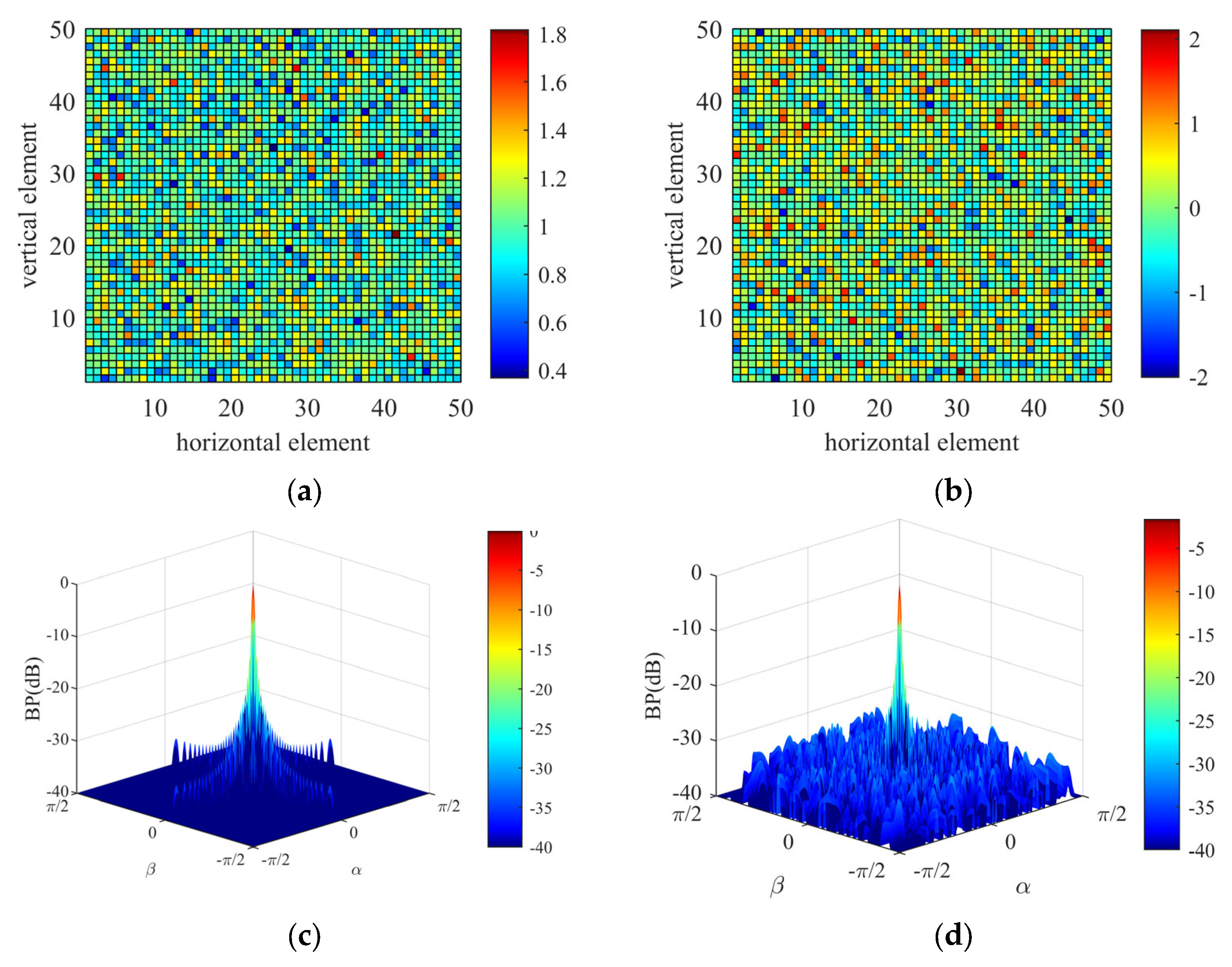
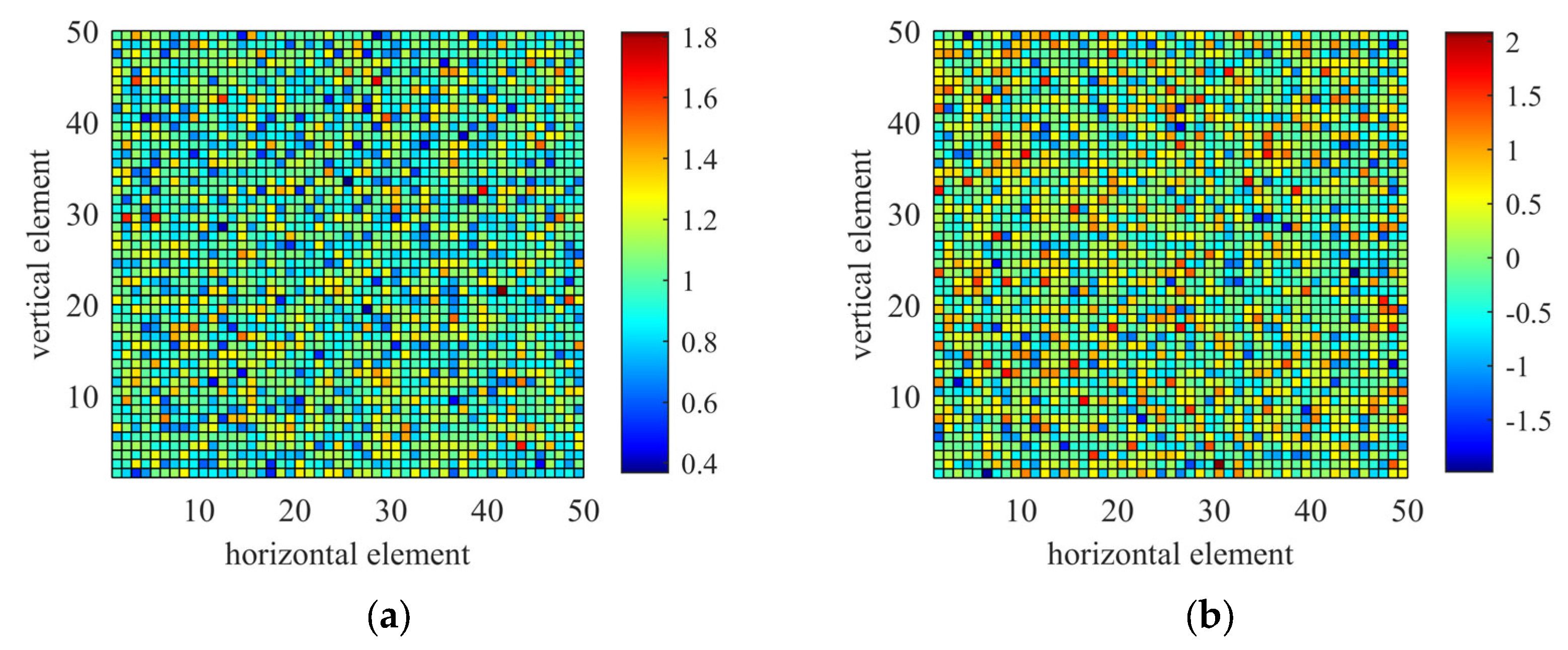
3.1. Calibration Performance of the Planar Array

The planar array calibration experiment used an array with 50 × 50 elements arranged at equal intervals with an element spacing of d = 2.5 mm. The calibration sound source signal frequency, f = 300 kHz, was in the far-field where distance r > ((M − 1)d)²c/f = 3 m, with the direction of the array as (10°, −20°). Additive Gaussian noise was used with an SNR of 20 dB and a signal sample length of L = 1000. In the experiment, the beam patterns were normalized to the main lobe intensity of the ideal array beam.

The error array after introducing random gain and phase errors of σ_ξ = 0.2 and σ_τ = 0.6 rad, respectively, is shown in Figure 3a,b. Owing to the gain and phase errors, a large number of chaotic side lobes appeared in the array beam pattern. Owing to the weakened directivity of the array caused by gain and phase errors, the intensity of the main lobe beam was slightly attenuated compared with the ideal case. The beam pattern deteriorated from Figure 3c,d, and the root mean squared error RMSE_BPe between the error array and ideal array beam patterns was 0.0112.

The estimated values of the gain and phase errors of the calibrated array after applying the proposed joint sparse estimation-based gain and phase error calibration method are shown in Figure 4. The estimated results for the array gain and phase errors were consistent with the actual values.

Table 1. Comparison of the actual and estimated values of the gain and phase errors of selected elements in the planar array.

Element Index	Gain Error Value (Normalized)			Phase Error Value (°)
	Error	Estimated	Estimation Bias	Error	Estimated	Estimation Bias
(5, 5)	1.0308	1.0278	−0.0030	−23.5977	−24.8616	−1.2639
(10, 10)	1.0584	1.0587	−0.0003	3.3011	2.0089	−1.2922
(15, 15)	0.8957	0.8983	0.0026	−28.7070	−26.9317	1.7743
(20, 20)	1.0154	1.0123	−0.0031	−53.0579	−51.3620	1.6959
(25, 25)	0.8333	0.8309	−0.0024	23.2944	23.2862	−0.0082
(30, 30)	1.4918	1.4877	−0.0041	−54.7659	−54.0988	0.6671
(35, 35)	1.1045	1.1024	−0.0021	19.9314	18.3286	−1.6027
(40, 40)	1.3969	1.3979	0.0010	−0.7911	0.3499	1.1410
(45, 45)	1.1263	1.1261	−0.0002	0.3017	−1.7904	−2.0921
(50, 50)	0.9297	0.9297	0.0006	−35.2634	−33.7776	1.4858

presents the actual values of the gain and phase errors on the array diagonal and the estimated results obtained using the proposed method. The maximum deviation in the gain error estimation is −0.0041, and the maximum deviation of the phase error estimation is −2.09°.

The calibration results were further evaluated by randomly selecting 10% of the array elements to calculate the differences between the actual and estimated values of the array gain and phase errors. The estimation bias distribution from the sampled elements is shown in Figure 5. For the array calibration estimation results, the maximum estimation bias of the gain error is −0.010, with 87.7% of the array elements having a gain error estimation bias within ±0.005, and RMSE_ξ = 0.0033. The maximum estimation bias of the phase error is −3.5°, with 84.5% of the array elements exhibiting a phase error estimation bias within ±2°, and RMSE_τ = 0.0242.

Array errors were corrected based on the error estimation results. The beam pattern of the calibrated array is presented in Figure 6a. The chaotic side lobes caused by array gain and phase errors were effectively suppressed after calibration. Figure 6b compares the array beam patterns, which is a horizontal beam slice with β = 0°. The beam pattern of the calibrated array was highly consistent with the ideal array beam pattern, and the normalized main lobe beam intensity exhibited negligible attenuation. The root mean squared error of the beam pattern was reduced to RMSE_BPc = 3.7509 × 10 ⁻⁴ after calibration.

3.2. Analysis of the Impact of the Gain Phase Error Value and Signal-to-Noise Ratio on the Performance of Array Calibration Methods

This section compares and analyzes the influence of key factors, such as gain and phase errors, and the SNR of the calibration signal, on calibration accuracy to further explore the performance of the proposed joint sparse estimation-based array calibration method under various conditions. A uniform planar array with 30 × 30 elements and an element spacing of 2.5 mm was used, with the calibration source placed in the far field of the array at (20°, 20°). By default, σ_ξ = 0.2, σ_τ = 0.25 rad, and SNR = 20 dB. In the experiments, 100 independent runs were conducted for each experimental condition to eliminate the influence of randomness, and the results were averaged. The experiment also included a comparison with the TSI [11] and CVX [17] methods, which perform well in calibrating uniform planar arrays.

The relationship between the error estimation accuracy and the standard deviation of the gain error σ_ξ of the array gain and phase error calibration methods, JSC and TSI, based on joint sparse estimation at σ_τ = 0.25 rad and SNR = 20 dB, is shown in Figure 7. Because the array gain error has a minimal impact on the signal angle estimation in the DOA estimation stage of the calibration signal, the RMSE of the gain and phase estimations of the three calibration methods remain stable when the array gain changes. As σ_ξ increases, the RMSE_ξ curve of the JSC method rises slightly; however, it remains generally lower than that of the TSI and CVX methods. The average RMSE_τ of the JSC method in all σ_ξ scenarios is 42% lower than that of the TSI method, and 45% lower than that of the CVX method.

Figure 8 illustrates the relationship between the array error estimation accuracy and the standard deviation of phase error, σ_τ, under the conditions of σ_ξ = 0.2 and SNR = 20 dB. Similarly to the ρ_ξ~RMSE_ξ experimental results, the change in RMSE_ξ is not significant as σ_τ increases. When σ_τ is less than 0.55 rad, the gain estimation error of the proposed JSC method is lower than that of the TSI method; when σ_τ is greater than 0.55 rad, it is slightly higher than the result of the TSI method; however, its average RMSE_ξ is 3.056 × 10⁻³, which is approximately 6% lower than the average estimation deviation of the TSI method. When σ_τ is less than 0.9 rad, the gain estimation error of the JSC method is lower than that of the CVX method, and its average RMSE_ξ is approximately 8% lower than the average estimation deviation of the CVX method. The phase error estimation accuracy of these calibration methods increases as σ_τ increases, and the growth is relatively rapid in the interval of σ_τ ∈ [0.7, 1] (Figure 8b). Because the estimation model combines the discrete grid points and continuous values used in the DOA estimation, The JSC method demonstrates higher stability against phase error interference, and its overall RMSE_τ remains lower than that of the TSI method, which uses frequency modulation estimation. In addition, when σ_τ is less than 0.9 rad, the phase estimation error of the JSC method is lower than that of the CVX method. Notably, although RMSE_τ increases rapidly when σ_τ exceeds 0.7 rad, its maximum does not exceed 0.015, and the performance degradation caused to the beam pattern is within an acceptable range. Moreover, in practical applications, the array phase error is typically controlled within 10° during manufacturing. Consequently, a situation where manufacturing errors or long-term use leads to σ_τ ≥ 0.7 rad (approximately ≥ 41°) is relatively rare.

The relationship between the SNR of the array response signal and the estimation accuracy of the gain and phase errors under the conditions of σ_ξ = 0.2 and σ_τ = 0.25 rad is shown in Figure 9. Unlike the previous experimental results for gain and phase errors (Figure 9a), the RMSE_ξ of gain error estimation is strongly correlated with the SNR, particularly at a low SNR, where RMSE_ξ increases by an order of magnitude. This is because when the SNR is low, the noise signal intensity is close to the calibrated signal intensity, making precise estimation in the DOA stage difficult and affecting the calibration accuracy. When the SNR ≥ 20 dB, the proposed JSC method can achieve higher estimation accuracy and outperform the other methods. In terms of the phase error estimation accuracy, both methods are relatively stable when the SNR ≥ 20 dB. As the SNR decreases further, the estimation accuracy decreases slightly. The JSC method consistently outperforms the other methods.

4. Discussion

The experiments demonstrate that, based on joint sparse estimation, the proposed array gain and phase-error calibration method achieves strong calibration performance across various scenarios. The gain and phase error and SNR experiments confirm that the proposed array calibration method maintains a high estimation accuracy even when the array error is large and performs stably in the conventional scenario where the SNR ≥ 20 dB, outperforming the comparison methods. The primary contributions of this study include: (1) A FISTA-based joint sparse DOA method is proposed, which combines discrete grid and continuous offset models, optimizing the gradient descent step size selection and nonlinear mapping to enhance the DOA estimation performance of the calibration signal. (2) Based on the linear array model, an iteration calibration signal processing framework and estimation model were proposed, extending the joint sparse estimation method to planar arrays and addressing the issue of the limited generalizability of the existing array calibration methods. (3) The influence of array phase errors on the DOA estimation of the calibration signal is corrected using ℓ_F and CVX, optimizing the estimation accuracy of phase errors.

In this study, a joint sparse estimation method for array calibration was developed based on FISTA. This method introduces a continuous off-grid migration matrix based on the sparse signal dictionary mismatch model and uses the Wolfe criterion to optimize the gradient step to accelerate the convergence. This involves jointly estimating the discrete direction and off-grid offsets to achieve DOA estimation with a high degree of freedom and accuracy without increasing the order of calculation. An iterative calibration signal processing framework was proposed, extending the method to planar arrays. Spatial filtering was employed to mitigate phase error interference in DOA estimation and to enhance the calibration accuracy of the array error. Moreover, the overall processing in the iterative process of joint sparse estimation may lead to ignoring the individual characteristics of signal samples. In addition, certain requirements must be met to ensure the stability of the calibrated source. Therefore, future studies and discussions on how to apply the joint estimation of multiple samples to the field of array calibration and optimize the robustness of the method are necessary.

References

1. Rockah, Y.; Schultheiss, P. Array shape calibration using sources in unknown locations–Part I: Far-field sources. IEEE Trans. Acoust. Speech Signal Process. 1987, 35, 286–299. [Google Scholar] [CrossRef]
2. Rockah, Y.; Schultheiss, P. Array shape calibration using sources in unknown locations–Part II: Near-field sources and estimator implementation. IEEE Trans. Acoust. Speech Signal Process. 1987, 35, 724–735. [Google Scholar] [CrossRef]
3. Rockah, Y.; Messer, H.; Schultheiss, P. Localization performance of arrays subject to phase errors. IEEE Trans. Aerosp. Electron. Syst. 1988, 24, 402–410. [Google Scholar] [CrossRef]
4. LI, Y.; ER, M.H. Theoretical analyses of gain and phase error calibration with optimal implementation for linear equispaced array. IEEE Trans. Signal Process. 2006, 54, 712–723. [Google Scholar]
5. Fuhrmann, D.R. Estimation of sensor gain and phase. IEEE Trans. Signal Process. 1994, 42, 77–87. [Google Scholar] [CrossRef]
6. Ng, B.C.; See, C. Sensor-array calibration using a maximum-likelihood approach. IEEE Trans. Antennas Propag. 1996, 44, 827–835. [Google Scholar]
7. Boonstra, A.J.; Van der Veen, A.J. Gain calibration methods for radio telescope arrays. IEEE Trans. Signal Process. 2003, 51, 25–38. [Google Scholar] [CrossRef]
8. Flanagan, B.P.; Bell, K.L. Array self-calibration with large sensor position errors. Signal Process. 2001, 81, 2201–2214. [Google Scholar] [CrossRef]
9. Roy, R.; Kailath, T. ESPRIT-estimation of signal parameters via rotational invariance techniques. IEEE Trans. Acoust. Speech Signal Process. 1989, 37, 984–995. [Google Scholar] [CrossRef]
10. Yuan, L.; Jiang, R.; Chen, Y. Gain and Phase Autocalibration of Large Uniform Rectangular Arrays for Underwater 3-D Sonar Imaging Systems. IEEE J. Ocean. Eng. 2014, 39, 458–471. [Google Scholar] [CrossRef]
11. Wang, F.; Jiang, R.; Tian, X.; Liu, X.; Jiang, S.; Gu, B.; Chen, Y. An Efficient Near-Field Model Gain-Phase Self-Calibration Method for Uniform Rectangular Arrays. IEEE J. Ocean. Eng. 2022, 47, 1129–1142. [Google Scholar] [CrossRef]
12. Wu, Y.; Rhodes, S.; Satorius, E.H. Direction of arrival estimation via extended phase interferometry. IEEE Trans. Aerosp. Electron. Syst. 1995, 31, 375–381. [Google Scholar]
13. Hou, Y.; Wang, W. Active Frequency Diverse Array Counteracting Interferometry-Based DOA Reconnaissance. IEEE Antennas Wirel. Propag. Lett. 2019, 18, 1922–1925. [Google Scholar] [CrossRef]
14. Florio, A.; Avitabile, G.; Coviello, G. A Linear Technique for Artifacts Correction and Compensation in Phase Interferometric Angle of Arrival Estimation. Sensors 2022, 22, 1427. [Google Scholar] [CrossRef]
15. Florio, A.; Bnilam, N.; Talarico, C.; Crosta, P.; Avitabile, G.; Coviello, G. LEO-Based Coarse Positioning Through Angle-of-Arrival Estimation of Signals of Opportunity. IEEE Access 2024, 12, 17446–17459. [Google Scholar] [CrossRef]
16. Terada, T.; Nishimura, T.; Ogawa, Y.; Ohgane, T.; Yamada, H. DOA Estimation for Multi-Band Signal Sources Using Compressed Sensing Techniques with Khatri-Rao Processing. IEICE Trans. Commun. 2014, 97, 2110–2117. [Google Scholar] [CrossRef]
17. Jie, X.; Zheng, B.; Gu, B. Gain and Phase Calibration of Uniform Rectangular Arrays Based on Convex Optimization and Neural Networks. Electronics 2022, 11, 718. [Google Scholar] [CrossRef]
18. Li, S.; Ma, Y.; Gao, Y.; Li, J. DOA Estimation Based on Bayesian Compressive Sensing. Wirel. Satell. Syst. PTI 2019, 280, 630–639. [Google Scholar]
19. Feng, X.; Zhang, X.B.; Song, R.P.; Wang, J.F.; Sun, H.X.; Esmaiel, H. Direction of arrival estimation under Class A modelled noise in shallow water using variational Bayesian inference method. IET Radar Sonar Navig. 2022, 16, 1503–1515. [Google Scholar] [CrossRef]
20. Ogut, M.; Bosch-Lluis, X.; Reising, S.C. Deep Learning Calibration of the High-Frequency Airborne Microwave and Millimeter-Wave Radiometer (HAMMR) Instrument. IEEE Trans. Geosci. Remote Sens. 2020, 58, 3391–3399. [Google Scholar] [CrossRef]
21. Wang, Y.; Yang, A.; Chen, X.; Wang, P.; Wang, Y.; Yang, H. A Deep Learning Approach for Blind Drift Calibration of Sensor Networks. IEEE Sens. J. 2017, 17, 4158–4171. [Google Scholar] [CrossRef]
22. Goodman, J.; Salmond, D.; Davis, C.; Acosta, C. Ambiguity Resolution in Direction of Arrival Estimation using Mixed Integer Optimization and Deep Learning. In Proceedings of the 2019 IEEE National Aerospace and Electronics Conference (NAECON), Dayton, OH, USA, 15–19 July 2019; pp. 317–322. [Google Scholar]
23. Ahmed, A.M.; Thanthrige, U.S.K.P.M.; El Gamal, A.; Sezgin, A. Deep Learning for DOA Estimation in MIMO Radar Systems via Emulation of Large Antenna Arrays. IEEE Commun. Lett. 2021, 25, 1559–1563. [Google Scholar] [CrossRef]
24. Wylie, M.R.; Roy, S.; Messer, H. Joint DOA estimation and phase calibration of linear equispaced (LES) arrays. IEEE Trans. Signal Process. 1994, 42, 3449–3459. [Google Scholar] [CrossRef]
25. Lin, Z.; Chen, Y.; Liu, X.; Jiang, R.; Shen, B. A Bayesian compressive sensing-based planar array diagnosis approach from near-field measurements. IEEE Antennas Wirel. Propag. Lett. 2020, 20, 249–253. [Google Scholar] [CrossRef]
26. Liu, H.; Zhao, L.; Li, Y.; Jing, X.; Truong, T. A sparse-based approach for DOA estimation and array calibration in uniform linear array. IEEE Sens. J. 2016, 16, 6018–6027. [Google Scholar] [CrossRef]
27. Sijtsma, P. CLEAN based on spatial source coherence. Int. J. Aeroacoustics 2007, 6, 357–374. [Google Scholar] [CrossRef]
28. Berestesky, P.; Attia, E.H. Sidelobe leakage reduction in random phase diversity radar using coherent CLEAN. IEEE Trans. Aerosp. Electron. Syst. 2019, 55, 2426–2435. [Google Scholar] [CrossRef]
29. Yang, T. Deconvolved conventional beamforming for a horizontal line array. IEEE J. Ocean. Eng. 2017, 43, 160–172. [Google Scholar] [CrossRef]
30. Zhou, T.; Huang, J.; Du, W.; Shen, J.; Yuan, W. 2-D Deconvolved conventional beamforming for a planar array. Circuits Syst. Signal Process. 2021, 40, 5572–5593. [Google Scholar] [CrossRef]
31. Mei, J.; Pei, Y.; Zakharov, Y.; Sun, D.; Ma, C. Improved underwater acoustic imaging with non-uniform spatial resampling RL deconvolution. IET Radar Sonar Navig. 2020, 14, 1697–1707. [Google Scholar] [CrossRef]
32. Wu, Q.; Fang, S. Structured Bayesian compressive sensing with spatial location dependence via variational Bayesian inference. Digit. Signal Process. 2017, 71, 95–107. [Google Scholar] [CrossRef]
33. Liu, J.; Wu, Q.; Amin, M.G. Multi-Task Bayesian compressive sensing exploiting signal structures. Signal Process. 2021, 178, 107804. [Google Scholar] [CrossRef]
34. Chu, Z.; Chen, C.; Yang, Y.; Shen, L.; Xi, C. Improvement of Fourier-based fast iterative shrinkage thresholding deconvolution algorithm for acoustic source identification. Appl. Acoust. 2017, 123, 64–72. [Google Scholar] [CrossRef]
35. Shen, L.; Chu, Z.; Tan, L.; Chen, D.; Ye, F. Improving the sound source identification performance of sparsity constrained deconvolution beamforming utilizing SFISTA. Shock Vib. 2020, 2020, 1482812. [Google Scholar] [CrossRef]
36. Xiang, J.; Dong, Y.; Yang, Y. FISTA-Net: Learning a fast iterative shrinkage thresholding network for inverse problems in imaging. IEEE Trans. Med. Imaging 2021, 40, 1329–1339. [Google Scholar] [CrossRef]
37. Chen, F.; Xiao, Y.; Yu, L.; Chen, L.; Zhang, C. Extending FISTA to FISTA-Net: Adaptive reflection parameters fitting for the deconvolution-based sound source localization in the reverberation environment. Mech. Syst. Signal Process. 2024, 210, 111130. [Google Scholar] [CrossRef]
38. Zhang, J.; Chu, P.; Liao, B. DOA Estimation in Impulsive Noise Based on FISTA Algorithm. Remote Sens. 2023, 15, 565. [Google Scholar] [CrossRef]
39. Liu, D.; Zhao, Y. Two-Dimensional DOA Estimation via Matrix Completion and Sparse Matrix Recovery for Coprime Planar Array. IEEE Trans. Veh. Technol. 2023, 72, 14127–14140. [Google Scholar] [CrossRef]
40. Beck, A.; Teboulle, M. Smoothing and first order methods: A unified framework. SIAM J. Optim. 2012, 22, 557–580. [Google Scholar] [CrossRef]
Figure 1. Calibration signal model for a uniform linear array.
Electronics 14 02165 g001
Figure 2. Calibration signal model for a uniform planar array.
Electronics 14 02165 g002
Figure 3. Ideal and error array beam patterns of the planar array and the gain and phase errors of the array: (a) error array gain error; (b) error array phase error; (c) ideal array beam pattern; (d) error array beam pattern.
Electronics 14 02165 g003
Figure 4. Estimation results of the gain and phase error of the calibrated planar array: (a) estimated array gain error; (b) estimated array phase error.
Electronics 14 02165 g004
Figure 5. Sampling distribution of deviation between the estimated and actual values of planar array calibration.
Electronics 14 02165 g005
Figure 6. Comparison of the beam patterns of the error, ideal, and calibrated planar array: (a) calibrated array beam pattern; (b) comparison of error, ideal, and calibrated planar array.
Electronics 14 02165 g006
Figure 7. Relationship between array calibration performance and gain error: (a) σξ and RMSEξ; (b) σξ and RMSEτ.
Electronics 14 02165 g007
Figure 8. Relationship between array calibration performance and phase error: (a) στ and RMSEξ; (b) στ and RMSEτ.
Electronics 14 02165 g008
Figure 9. Relationship between array calibration performance and SNR: (a) SNR and RMSEξ; (b) SNR and RMSEτ.
Electronics 14 02165 g009