Adaptive Threshold Wavelet Denoising Method and Hardware Implementation for HD Real-Time Processing

Abstract

To meet the demands of real-time and high-definition (HD) image processing applications, denoising methods must be both computationally efficient and hardware friendly. Traditional image denoising techniques are typically simple, fast, and resource-efficient but often fall short in terms of denoising performance and adaptability. This paper proposes an adjustable-threshold denoising method along with a corresponding hardware implementation designed to support the real-time processing of large-array images commonly used in image signal processors (ISPs). The proposed technique employs a LeGall 5/3 wavelet with a row-transform structure and multilevel decomposition. A 2D Pyramid VisuShrink thresholding algorithm is introduced, where the threshold is derived from the median value of the HH sub-band using a multi-stage segmentation approach. To further optimize performance, a quantization strategy with fixed-point parameter design is applied to minimize storage requirements and computational errors. A specialized hardware architecture is developed to enable the real-time denoising of 4K images while adhering to constraints on speed and resource utilization. The architecture incorporates a finite state machine (FSM) and a reusable median calculation unit to efficiently share threshold-related storage and computational resources. The system is implemented and verified on an FPGA, achieving real-time performance at a maximum frequency of 230 MHz. It supports flexible input data formats with resolutions up to 4096×4096 pixels and 16-bit depth. Comprehensive comparisons with other real-time denoising methods demonstrate that the proposed approach consistently achieves better PSNR and SSIM across various noise levels and image sizes. In addition to delivering improved denoising accuracy, the hardware implementation offers advantages in processing speed and resource efficiency while supporting a wide range of large-array images.

1. Introduction

An image signal processor is an indispensable technology for high-definition image acquisition [1]. By performing operations such as denoising, enhancement, and correction at the terminal stage, ISPs significantly improve image quality and clarity, laying the foundation for advanced applications like object recognition and tracking. The growing demand in fields such as security monitoring [2], biomedical image enhancement [3], and aerospace [4] highlights the need for ISPs that can handle not only low-resolution quasi-static images but also high-resolution, real-time data streams. While medical imaging requires high-definition clarity for accurate diagnoses, the scale and scope of security and remote sensing applications often demand even more detailed, large-scale images, particularly in scenarios like surveillance and aerospace. Noise remains a significant challenge during real-time image acquisition, transmission, and processing. As a result, extensive research has been dedicated to developing effective methods for noise reduction to preserve visual quality and critical details.

Aiming at the illustrated problem above, real-time image denoising in ISPs face several key issues. First, noise levels are influenced by various environmental factors such as gain control, ambient temperature, and optical signal intensity. As a result, an adaptive denoising method with automatic threshold adjustment is essential to accommodate different imaging conditions. ISPs are characterized by high readout rates, so the chosen denoising method must support real-time processing without introducing significant latency. Third, the real-time processing of high-resolution, high-precision images imposes stringent requirements on hardware implementation due to the limited computational and memory resources available in ISP systems. This requires a reduction in hardware complexity, while maintaining algorithmic accuracy, especially for larger, high-definition images typical of security monitoring and remote sensing scenarios.

For real-time HD image processing systems constrained by latency and resource limitations, signal filtering methods [5,6,7] are generally more suitable for ISP implementations than other common approaches. These algorithms contain statistical-model-based estimation [8], Wiener filtering [9], a subspace method [10], a median filter [11], a bilateral filter [12], and a wavelet filter [13]. Among them, wavelet denoising stands out as an adjustable-threshold method [14] that enables the precise analysis of images in both the time [15] and frequency domains. This capability enhances detail preservation and makes the approach well suited for high-quality denoising. Additionally, wavelet-based methods are relatively straightforward to implement in hardware, making them an optimal choice for real-time preprocessing in ISP systems compared to other filtering techniques.

The research on wavelet denoising mainly focuses on model-based methods, learning-based approaches, and hardware-efficient implementations. In the category of wavelet-based model-driven denoising, refs. [16,17,18] effectively remove noise and retain the image details by using wavelet decomposition. Compared with traditional filters, wavelet transform filters can significantly improve image quality indicators. Meanwhile, some methods introduce adaptive mechanisms, reducing the dependence on manual parameter settings. However, these methods have certain limitations, such as regarding the adaptability to noise types, computational complexity, and the narrow scope of experimental verification. Their generalizability and practicability need to be further strengthened. Ref. [19] proposes a wavelet-domain-style transfer method that uses 2D stationary wavelet transform and an enhanced network, aiming to achieve a better perception–distortion trade-off in regard to super-resolution imaging. Deep learning and wavelet co-design frameworks have attracted research attention. Refs. [20,21] effectively combine wavelet transform with deep learning networks, which can achieve strong robustness and better detail restoration ability in image super-resolution and denoising tasks. However, such methods generally involve problems, such as high computational complexity, large resource consumption, a complex network structure, and high implementation difficulty, which limit their deployment and application in practical scenarios. Wavelet denoising accelerators, based on the FPGA platform, were designed in [22,23], which made full use of hardware parallelism. A wavelet denoising accelerator outperformed other methods in improving the processing speed, reducing delays, and achieving low-power consumption [24]. These methods generally involve high resource utilization and complex design and implementation structures, and most of the architectures are applicable to medical fields, such as ECGs [25]. The image size is very small and not suitable for high-definition image processing, which restricts their promotion in a wider range of application scenarios. As a consequence, advanced denoising algorithms offer excellent performance, but their complexity limits hardware deployment. Existing hardware-oriented designs often lack adaptive thresholding and are unsuitable for high-definition processing. Thus, efficient real-time denoising methods for high-definition images balancing performance, adaptability, and hardware feasibility remain largely unexplored.

This paper presents a real-time adaptive wavelet denoising algorithm and its hardware implementation method. We propose an improved wavelet domain adaptive threshold algorithm based on the VisuShrink threshold and put forward a quantization optimization strategy for hardware implementation. The key parameters and fixed-point calculations are finely designed to minimize storage overhead and calculation errors. On the basis of maintaining the denoising performance of the original algorithm, this method has a better effect compared with the traditional filtering algorithm. In addition, a dedicated hardware architecture is proposed for large-format 4K video stream processing, integrating LeGall 5/3 wavelet transform, reusable median computing units, and sequencing multiplexing circuits based on finite state machines. Under the conditions of resource constraints and high-speed processing requirements, real-time adaptive denoising of large-area array images is achieved. This text also presents a comparative analysis of the denoising effect and the cost of hardware resources, verifying the efficiency and practical value of the proposed method.

2. Adaptive Wavelet Denoising Algorithm

The architecture of the adaptive threshold wavelet denoising algorithm is shown in Figure 1, including wavelet denoising and threshold calculation. The system consists of three main stages: wavelet decomposition, denoising, and wavelet reconstruction. Lifting-based LeGall 5/3 transforms are used for efficient wavelet decomposition and reconstruction. In the denoising module, soft thresholding is applied to high-frequency coefficients, with an adaptive threshold computed based on an efficient median calculation algorithm suitable for hardware implementation. Two-stage wavelet decomposition is adopted to balance denoising performance and hardware costs.

2.1. Wavelet Denoising

The lifting Legall 5/3 basis [26] is used to implement the Mallat wavelet transform, offering advantages in computational efficiency and reduced storage requirements, which make it well-suited for hardware implementation. The lifting scheme consists of three main steps: splitting, prediction, and updating. The splitting process decomposes the original image pixel x_i into the odd set x_i,2l+1 and even set x_i,2l. The lifting operators are applied to obtain the residual signal d_i and low-frequency coefficients s_i. The above calculations are shown in (1)–(4).

$$s_i^{(0)}=x_{2l}$$

(1)

$$d_i^{(0)}=x_{2l+1}$$

(2)

$$d_i^{(1)}=d_i^{(0)}+⌊-{\displaystyle \frac{1}{2}}\times \left(s_i^{(0)}+s_{i+1}^{(0)}\right)+{\displaystyle \frac{1}{2}}⌋$$

(3)

$$s_i^{(1)}=s_i^{(0)}+⌊{\displaystyle \frac{1}{4}}\times \left(d_i^{(0)}+d_{i+1}^{(0)}\right)+{\displaystyle \frac{1}{2}}⌋$$

(4)

In two-dimensional wavelet decomposition, the image is first processed by row-wise transforms to separate it into low- and high-frequency components. A subsequent column-wise transform further divides the result into four sub-bands, named LL, LH, HL, and HH. For multilevel decomposition, this operation is recursively applied to the LL sub-band. A soft threshold is adopted for denoising [27], and the high-frequency coefficients w_i,j below an appropriate threshold TH are set to zero; others are retained or attenuated. The estimated coefficients are calculated in (5).

$${\widehat{w}}_{i,j}=\left\{\begin{array}{c}sign\left(w_{i,j}\right)\times \left(\left|w_{i,j}\right|-TH\right)\hspace{1em}\hspace{1em}\hspace{1em}\left|w_{i,j}\right|\ge TH\\ \hspace{1em}\hspace{1em}\hspace{1em}\hspace{1em}\hspace{1em}0\hspace{1em}\hspace{1em}\hspace{1em}\hspace{1em}\hspace{1em}\hspace{1em}\left|w_{i,j}\right|<TH\end{array}\right.$$

(5)

VisuShrink [28] is used as the adaptive threshold method, while L stands for signal length and $\sigma$ stands for standard deviation. The threshold calculation and estimation of are shown in (6) and (7).

$$TH=\sigma \sqrt{2\times \log \left(L\right)}$$

(6)

$$\widehat{\sigma }={\displaystyle \frac{median\left|HH\right|}{0.6745}}$$

(7)

The wavelet stage is a critical factor in denoising performance. We use multi-stage wavelet transforms of 1-dwt, 2-dwt, and 3-dwt to test images. From lots of experiments, the results show that 1-DWT provides limited denoising capability, while 3-DWT introduces noticeable blurring and distortion, in addition to significantly increasing hardware storage requirements. In contrast, 2-DWT achieves a good balance between noise reduction and edge preservation; thus a two-level decomposition is selected as the optimal configuration for our denoising approach.

2.2. Median Calculation

As shown in (6), calculating the median value of the entire HH sub-band is required. Due to limited hardware resources, this operation poses challenges for real-time implementation. Thus, we propose an improved median calculation algorithm suitable for real-time processing to solve this problem.

Assume the HH sub-band has a size of n × n. For each row containing n × n pixels, a segment of m pixels is extracted and defined as a Median Sort (MS) Unit. All MS Units within a row constitute the first group for intermediate median calculation. The median value of each MS Unit is computed and stored in a continuous memory block, forming the second group. These stored values are then reorganized into new MS Units, each again containing mmm elements, and the process is repeated. Let (8) denote the median value of each unit, where i denotes the current row, j denotes the current MS Unit, and k denotes the current group. From several iterations, a one-dimensional row median array of length n is generated for each row. Each element of this array is represented by (9), with i indicating the row index. To obtain the final median of the HH sub-band, the same iterative median calculation process is applied column-wise to the row median arrays. From the discussion above, the number of MS Unit groups required for each row can be calculated using (10). The total number of median operations, denoted as F, is given by (11). An overview of the algorithm is illustrated in Figure 2.

$$\left\{{\chi }_{i,j}^{\left(k\right)}\left|i\in \left[1,n\right],j\in \left[1,⌊{\displaystyle \frac{n}{m}}⌋\right],k\in \left[1,g\right]\right.\right\}$$

(8)

$$\left\{{\chi }_i|i\in [1,n]\right\}$$

(9)

$$g=⌈{\log }_{m}n⌉$$

(10)

$$F=\left(⌈n\times m^{-1}⌉+\cdots +⌈n\times m^{-\left(g-1\right)}⌉+⌈m^{-g}⌉\right)\times \left(n+1\right)$$

(11)

It must be noted that the number of pixels in an MS Unit is not always m. We regard m′ as the actual pixel number of an MS Unit; the case of m′ < m regularly occurs in the last MS Unit of each row. We define that the median value is calculated by the number of m′ pixels as 1 < m′ < m; otherwise, the MS Unit will be discarded in the case of m′ = 1, and m′ is not the row median value. The above definition is detailed in (12).

$$median(w_1,\dots ,w_{m\prime })=\left\{\begin{array}{c}median(w_1,\dots ,w_m)\hspace{1em}\hspace{1em}m\prime =m\\ median(w_1,\dots ,w_{m\prime })\hspace{1em}\hspace{1em}m\prime <m\\ \hspace{1em}\hspace{1em}NaN\hspace{1em}\hspace{1em}\hspace{1em}\hspace{1em}m\prime =1\end{array}\right.$$

(12)

In the calculation process, the selection of segment parameter m will greatly affect the result of the threshold. According to the feasibility of hardware implementation, three m values of 9, 16, and 25 are used for the comparison. A total of 100 matrices with a size of 2048 × 2048 are generated randomly to imitate a number of HH sub-bands of 4096 × 4096 images. We define the original median value $\chi$ and the estimated median value $\widehat{\chi }$, and then the normalized error η can be defined as (13). The histogram statistics of η are shown in Figure 3, and the calculation result of m = 16 is better than other options. Theoretically, the situation of m′ < m of the 4096 × 4096 images is less likely to occur as m = 16, so the approximate result is closest to the original value. Thus, m = 16 is selected as the piecewise parameter.

$$\eta ={\displaystyle \frac{\left|\chi -\widehat{\chi }\right|}{\chi }}$$

(13)

3. Hardware Implementation

3.1. Architecture of Wavelet Transform

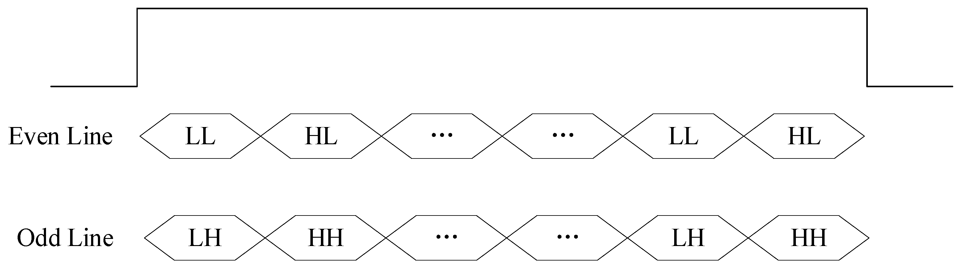
Since wavelet transform operates in both row and column directions, the lifting steps must be applied accordingly in both dimensions. On account of the large scale of the images, a multilevel decomposition structure based on row transformation is adopted. As illustrated in Figure 1, a row of input image data is first separated into odd and even line buffers, and a lifting-based row filter is applied. The coefficients for column filtering are then obtained by progressively applying vertical filtering to the results of the row processing. This structure significantly reduces the need for intermediate data storage. By utilizing only a small number of line buffers, it enables a pipelined line decomposition mode, allowing both row and column filtering to be completed in a single image data pass. For the filtering operations, only two additional row memories are required. The sub-band data output structure is shown in Figure 4. Because two rows of data are processed simultaneously, the computational units achieve 100% hardware utilization [29]. The architecture includes two dedicated filters that handle the first and second stages of the wavelet transform independently, ensuring efficient multilevel decomposition with minimal resource overhead.

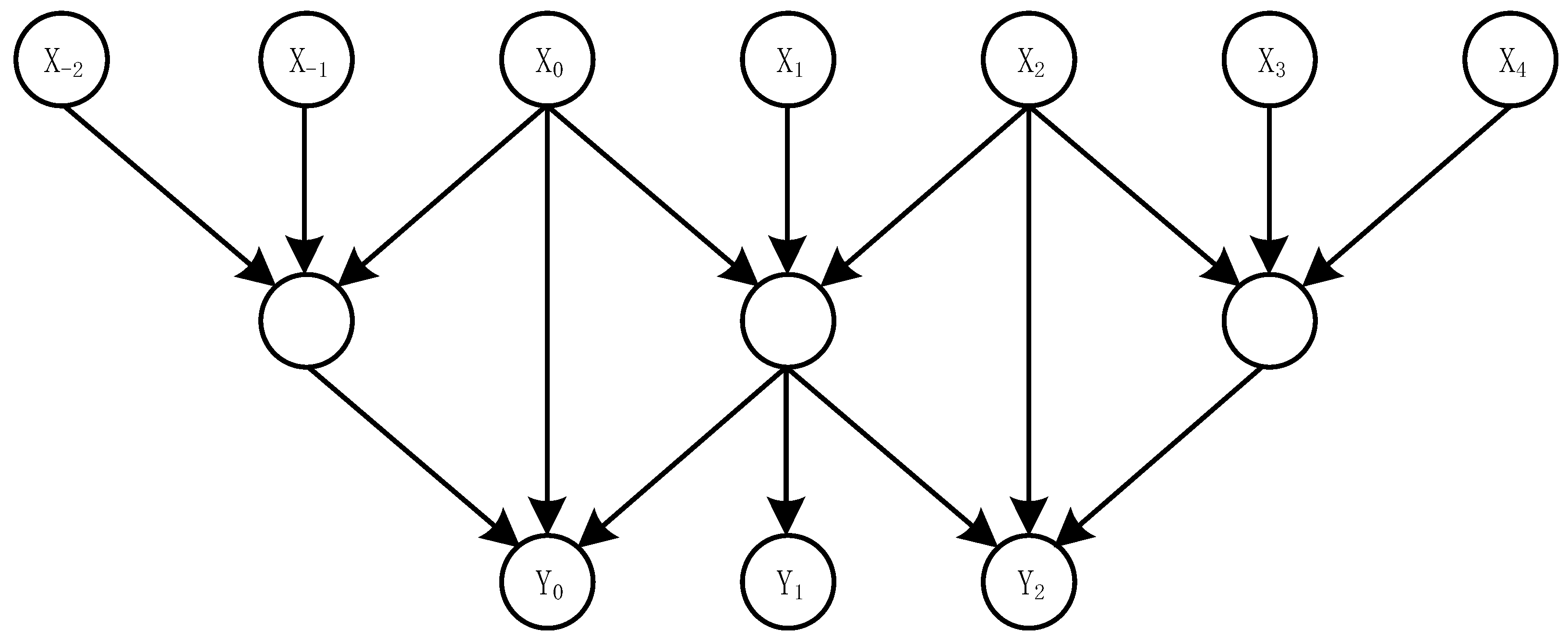
In the LeGall 5/3 lifting wavelet transform, boundary conditions are handled using symmetric extension, where the edge pixels are mirrored to provide the necessary data for prediction and update operations. Specifically, for the 5/3 wavelet, two pixels are extended on the left boundary and one pixel on the right boundary, as illustrated in Figure 5.

The memory usage in the processing system is primarily allocated for wavelet transforms and the storage of coefficients used in threshold calculation. The detailed memory requirements are as follows: During the first wavelet decomposition, a row of input data is split into odd and even components, which requires one line buffer. The 1-DWT column transform then needs two additional line buffers for the lifting operation. After completing the 1-DWT, the resulting LL sub-band must be cached for the second-level wavelet transform, which requires another two line buffers. Additionally, after each filtering stage, the output data must be aligned across rows, necessitating one further line buffer. This process is repeated in the i-DWT transform, following a similar memory usage pattern. Thanks to the multilevel decomposition structure based on row-wise data processing, memory consumption is minimized. Furthermore, the threshold calculation is designed to utilize existing storage resources, eliminating the need for additional memory allocation.

3.2. Threshold Calculation Design

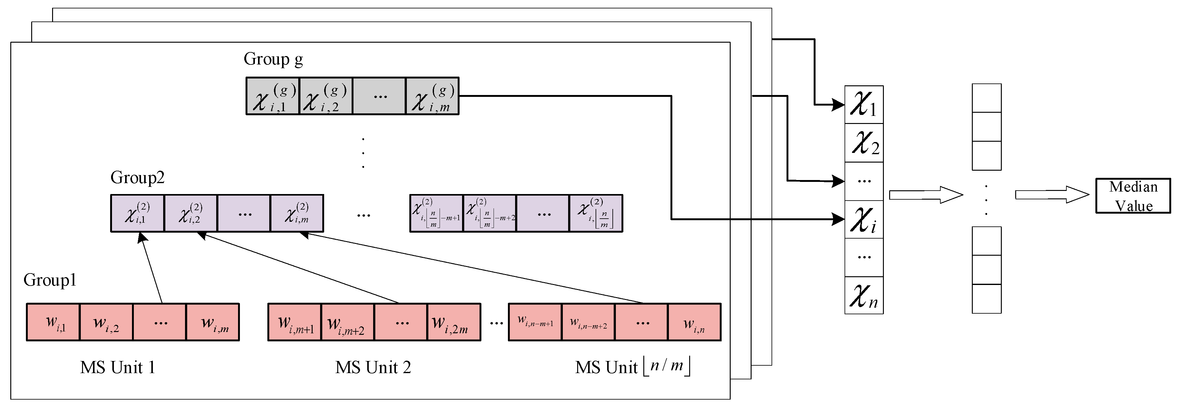
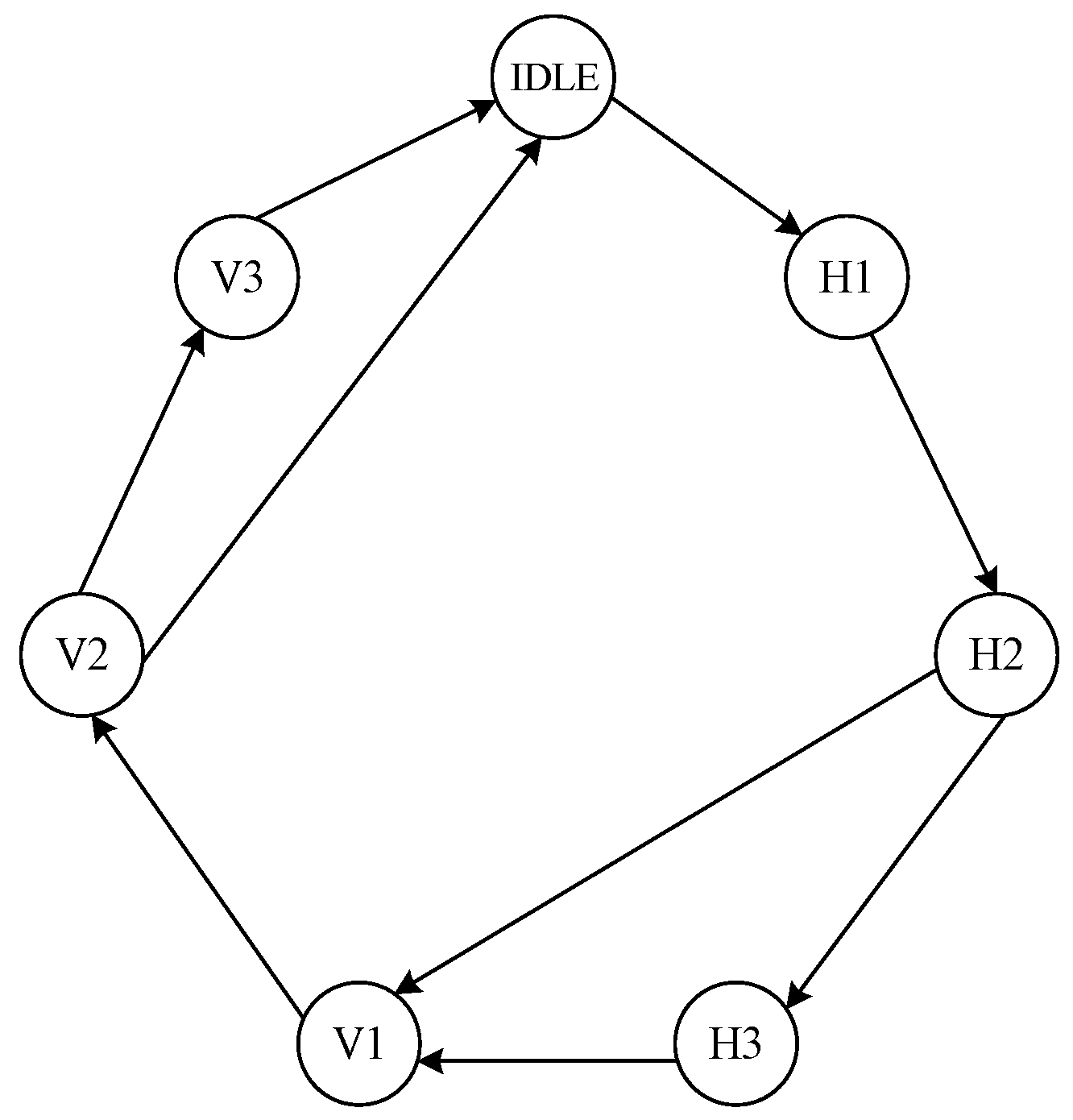
Since the median calculation needs to be piecewise, an FSM shown in Figure 6 is defined to distinguish the current state of the circuit. Taking a 4096 × 4096 image as an example, according to (10), three groups are needed to calculate the median value of a row. The first group is calculated to obtain 128 median values, and the calculation process is regarded as state H1. The second group calculates 8 median values from 128 data of the first group results, which is regarded as state H2. The third group is the special case of m′ < m, and the row median value is calculated by eight intermediate results, which is regarded as state H3. The states of V1, V2, and V3 are needed to calculate the column median values in the same way. Therefore, seven switching states are needed during the median calculation to obtain the final median value. For smaller images, H3 and V3 states may not be required, and the corresponding computing units will be reduced as well. 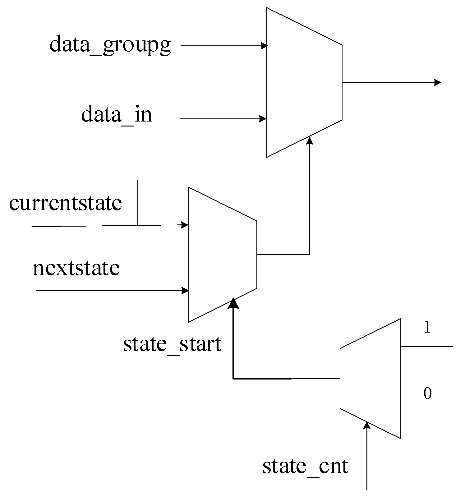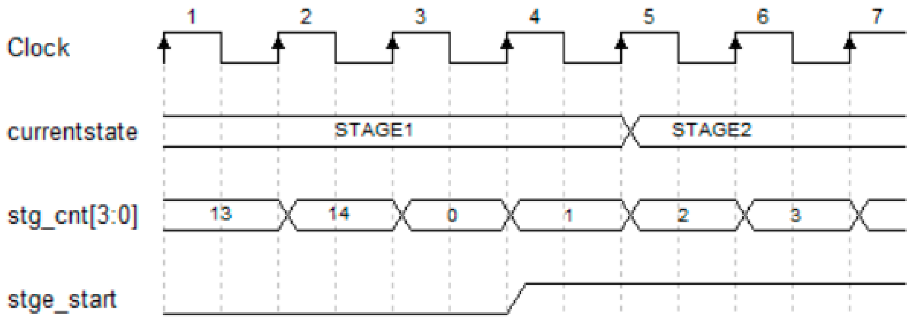The circuit structure is shown in Figure 7. The control signal of the state switch is determined by the current state and counters. As the counter reaches the maximum value, the corresponding state start signal jumps to a high level, and the state transmits from the current state to the next state. As Figure 6 shows, three multiplexers are used to select the appropriate state start signal, state signal, and input data. The control signals and counters used for the state switch are shown in Figure 8.

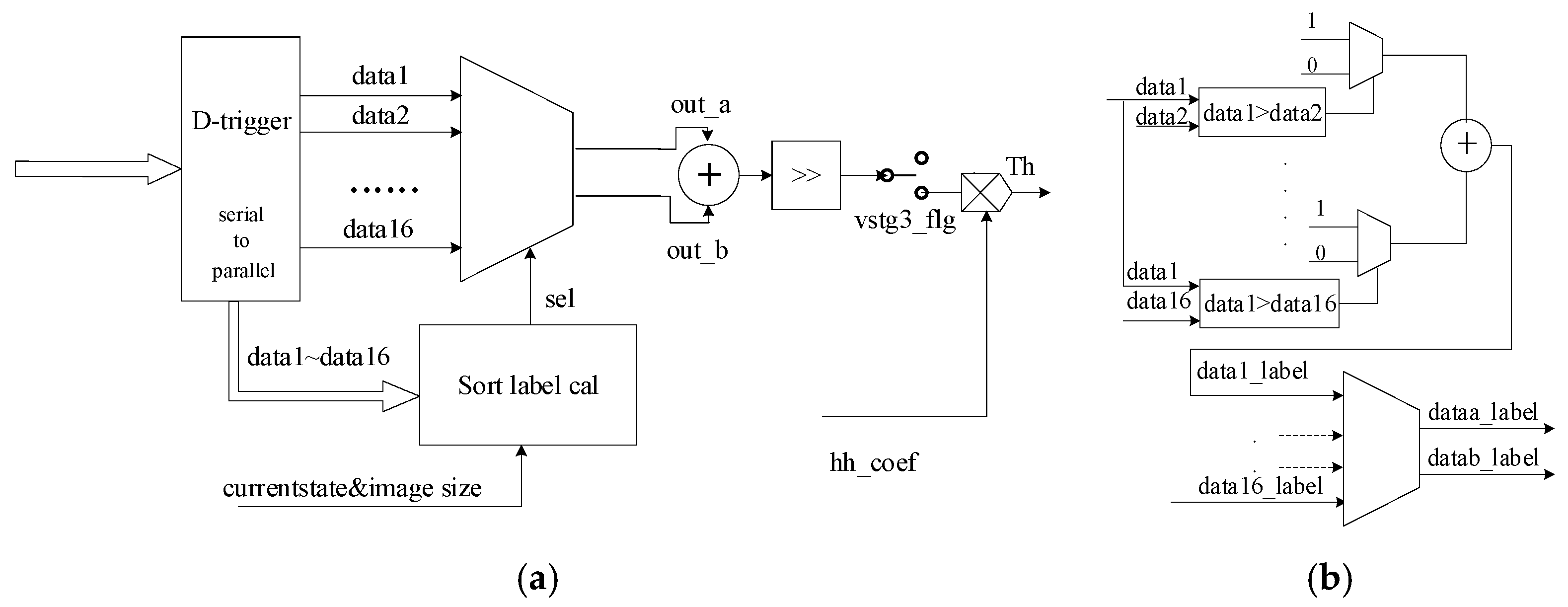
We adopt the parallel sorting method for the internal design of MS Units, and the architectures are shown in Figure 9. The serial unit pixels are transformed into a parallel structure. Pairwise comparisons of every two pixels are executed in parallel by D-trigger. Corresponding latency is reduced by the parallel structure, whereas additional registers are needed to store intermediate results. As in Figure 9b, every two pixels are compared and added together as a sorting label to represent the order of pixels. The same procedures are repeated, resulting in sorting labels of 16 pixels in MS Units. A multiplexer is used to select the pixels as median values, of which the label values are 7 and 8.

Similar to Section 2.2, we need to discuss the special case of m’ < m. We propose a reuse circuit to change the mapping regulation of the multiplexer instead of redesigning the sorting circuit. The mapping guideline is mainly determined by the FSM current state and image size. For example, if the current state of FSM is H3 and the image size is 4096 × 4096, then m′ = 8. The values in MS Units with sorting labels 4 and 5 are mapped as median values. A mapping table designed is applied to the multiplexer to convert the special condition into a general case, which increases the reuse ratio and complexity reduction. An adder and a shifter are applied to the selected pixels to obtain the median value ${\chi }_{x,j}^{\left(k\right)}$.

For the threshold TH, we define two constant parameters of two stages during initialization in (14). The threshold can be obtained by a multiplier in (15).

$$\begin{array}{l}hh\_coef1={\displaystyle \frac{\sqrt{2\log (\frac{hsize}{2}\times \frac{vsize}{2})}}{0.6745}}\\ hh\_coef2={\displaystyle \frac{\sqrt{2\log (\frac{hsize}{4}\times \frac{vsize}{4})}}{0.6745}}\end{array}$$

(14)

$$TH=hh\_coefx\times median$$

(15)

3.3. Accuracy and Storage Estimation

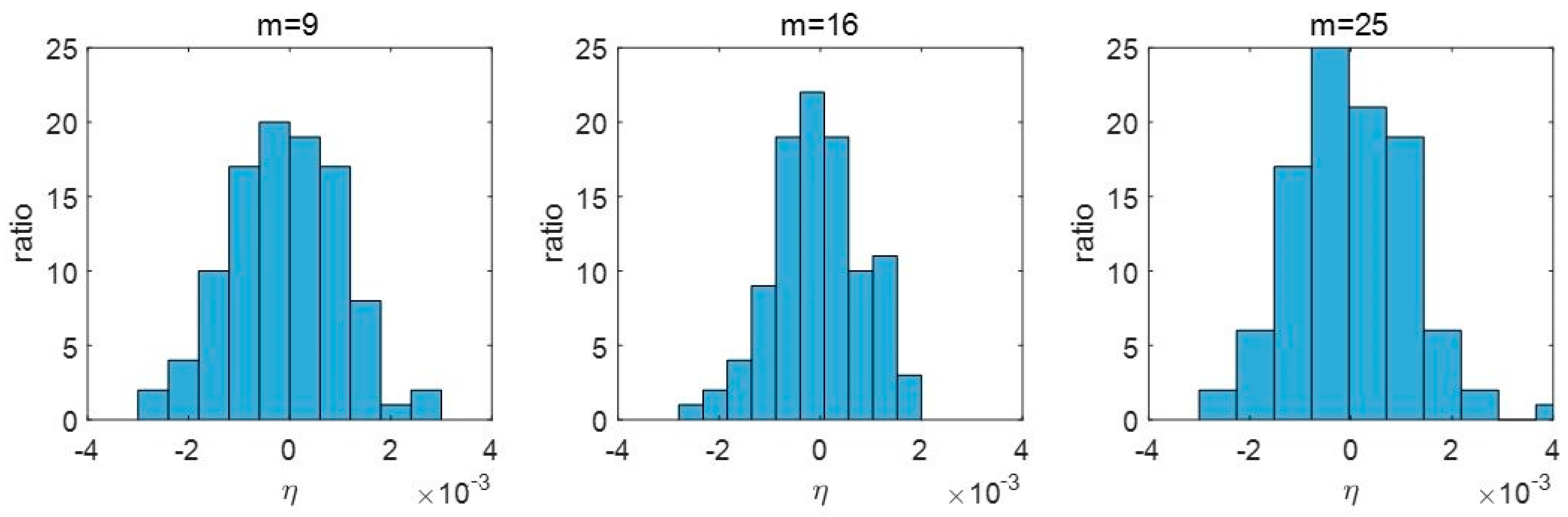
For hardware-based wavelet computation, a lossless transformation is adopted to preserve signal integrity. A fixed-point design is generally adopted, ensuring sufficient bit width in register initialization to maintain accuracy and prevent overflow during processing. According to experimental verification, the input data are expanded by 3 bits prior to wavelet decomposition to guarantee a lossless transform. Therefore, the LL sub-band retains 19-bit registers after wavelet transform, and the HL, LH, and HH sub-bands retain 17-bit registers. For the inverse wavelet reconstruction, an additional 3-bit extension is applied, resulting in the use of 22-bit registers to further safeguard against overflow. In the process of threshold calculations, 6 decimal bits are retained in the median calculation, and 9 fractional bits are preserved in the HH coefficients. Finally, during the threshold multiplication, only the integer part of the result is retained to complete the fixed-point operation. The results of 1-DWT threshold calculations across test images are presented in

Table 1. Accuracy of threshold implementation.

Image	Algorithm Threshold	Implementation Threshold
lena	13.9648	13
Castle	7.8038	7
Great_wall	2.0469	2

, showing no variation in the integer parts of the computed thresholds. Since wavelet coefficients are inherently integers, the fixed-point approximation introduces only minimal error, validating the suitability of the proposed hardware design.

3.4. FPGA Verification

The method is verified based on the Genesys 2 FPGA development board (Digilent Inc., Pullman, WA, USA), which is equipped with Xilinx Kintex-7 chip (Xilinx Inc., San Jose, CA, USA), in cooperation with Xilinx’s development suite Vivado 2018.3. Since the test images are too large to be directly stored in in-chip RAM, 4096 × 4096 × 16 bit images need to be stored on an SD card and then loaded into DDR SDRAM after power on. The data are read out according to a specified time sequence by DDR rules to start the denoising process. In addition, on-board hardware resources are required for validation, including a VGA monitoring interface for viewing image processing effects and a UART interface for data export comparison.

The verification process is as follows: after power-on reset, the image data on the SD card are transmitted to DDR through the SPI interface, and the image data are read out from DDR in accordance with a specified frequency and processed inside the FPGA. The output data are read out by the UART for comparison and enter the “Resize Module” for sampling. The resize data are displayed on VGA monitoring for observation. The denoising effect can be reproduced on the hardware platform, and the timing synthesis has no illegal situation.

In hardware design, only 56 BRAMs are used throughout the entire processing pipeline, which is quite economical considering the 4K image size. Resource consumption including slices, LUTs, and BRAMs is kept around 10% of the available resources, ensuring high efficiency and integration potential. The system achieves a maximum clock frequency of 230 MHz, with the critical path located at the interface for image data input, and the worst negative slack reported is 2.055 ns. Despite supporting high-resolution real-time processing, the total power consumption is only 931 mW, reflecting the low-power and lightweight characteristics of the architecture. DSP usage is also minimized; the adaptive thresholding module employs only a single multiplier, highlighting the efficiency and compactness of the designs.

4. Performance Evaluation

4.1. Denoising Effect

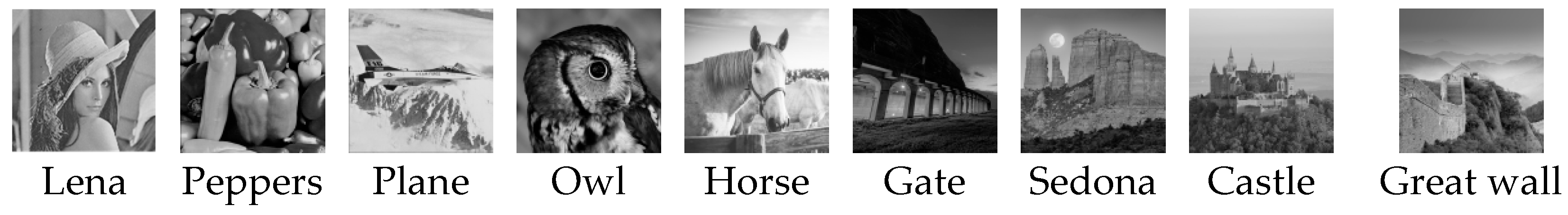
The proposed method is compared with filtering algorithms including TG Median Filter [30], db2 filter [31], bilateral filter [32], and contourlet filter [33]. We choose nine test images shown in Figure 10 of different sizes: 512 × 512, 1024 × 1024, and 4096 × 4096. Considering that application scenarios such as infrared, low-light, and biomedical images are mainly based on grayscale images, we use grayscale images as test cases. Mixed noises of gaussian, speckle, and Poisson are added to the images, the variances are 0.01, 0.02, and 0.03, and different noise levels are added for each image size for a comprehensive contrast.

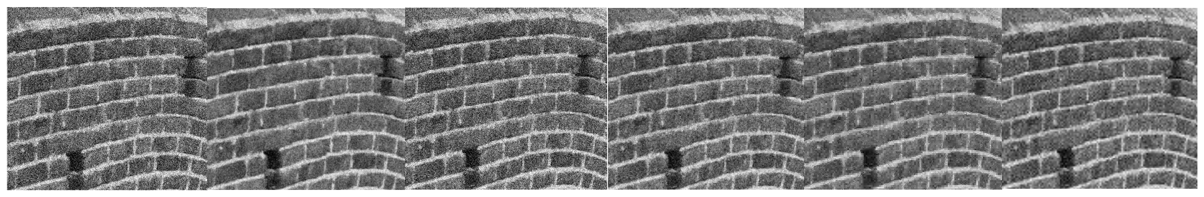
Figure 11 shows the experimental performance of different algorithms. Our method has better visual effects, especially the conditions of larger noise variance. The standard evaluation indexes of image quality including PSNR [34] and SSIM [35] are shown in

Table 2. The quantitative comparison between denoising algorithms in terms of PSNR.

Image	Size	σnoise	Noise Image	TG Median Filter [30]	Db2 Filter [31]	Bilateral Filter [32]	Contourlet [33]	Ours
Lena	512 × 512	0.01	18.31	25.46	19.06	26.78	24.55	27.07
Peppers	512 × 512	0.02	16.32	23.25	16.79	23.69	22.80	24.94
Plane	512 × 512	0.03	14.32	20.91	14.62	20.73	20.13	22.94
Owl	1024 × 1024	0.01	19.16	26.32	20.09	27.80	25.78	28.16
Horse	1024 × 1024	0.02	15.91	22.32	16.35	22.71	22.65	23.99
Tiger	1024 × 1024	0.03	14.62	20.70	14.94	20.63	20.05	22.06
Sedona	4096 × 4096	0.01	18.82	26.26	19.68	27.68	26.32	28.22
Castle	4096 × 4096	0.02	16.02	23.06	16.48	23.73	24.26	26.02
Great wall	4096 × 4096	0.03	14.41	21.74	14.73	21.28	22.42	25.41

and

Table 3. The quantitative comparison between denoising algorithms in terms of SSIM.

Image	Size	σnoise	Noise Image	TG Median Filter [30]	Db2 Filter [31]	Bilateral Filter [32]	Contourlet [33]	Ours
Lena	512 × 512	0.01	0.19	0.45	0.21	0.55	0.47	0.65
Peppers	512 × 512	0.02	0.16	0.37	0.17	0.43	0.43	0.56
Plane	512 × 512	0.03	0.14	0.31	0.14	0.31	0.30	0.49
Owl	1024 × 1024	0.01	0.20	0.49	0.23	0.60	0.54	0.68
Horse	1024 × 1024	0.02	0.12	0.29	0.13	0.36	0.42	0.53
Tiger	1024 × 1024	0.03	0.17	0.32	0.18	0.37	0.35	0.47
Sedona	4096 × 4096	0.01	0.18	0.48	0.20	0.58	0.52	0.65
Castle	4096 × 4096	0.02	0.10	0.31	0.11	0.36	0.42	0.53
Great wall	4096 × 4096	0.03	0.05	0.22	0.06	0.22	0.32	0.50

, and the result is consistent with the visual effect. From the data, we can see that in the case of small noise variance, the performance of our method is slightly better than other methods compared with TG median filter and bilateral filter. The difference is more obvious in high-noise-variation pictures. As noise variance equals 0.03, the contourlet filter has the best effect in the comparison scheme, but there is still a big gap with our method. This is attributed to the good self-adaptability of our method. The accuracy of threshold calculation design, as well as the detail retention capability and self-adaptability of the wavelet domain, are also the reasons for the good evaluation effect.

To evaluate the impact of quantization and fixed-point operations, we conducted additional experiments comparing the PSNR and SSIM values of original computation and quantitative operation using the same LeGall 5/3 wavelet basis. The results show no measurable difference in PSNR and SSIM across various test images, indicating that the quantization and bit-width design did not introduce any observable degradation. This confirms that our fixed-point architecture maintains denoising performance while achieving hardware efficiency and low resource consumption.

Figure 12 shows the denoised image details. TG median filter [30] performs best in preserving edges and contour structures, while our method introduces slight edge blurring but offers stronger noise suppression. To assess the preservation of the image structure, we adopt the FSIM metric for evaluation.

As shown in

Table 4. The quantitative comparison between denoising algorithms in terms of FSIM.

Image	Noise Image	TG Median Filter [30]	Db2 Filter [31]	Bilateral Filter [32]	Contourlet [33]	Ours
Great wall	0.9791	0.9894	0.9792	0.9801	0.9806	0.9806

, the TG median filter [30] achieves the highest FSIM score, primarily due to its strong edge-preserving capability. Since FSIM is highly sensitive to phase congruency and gradient information, algorithms that retain sharp edges and fine structural details tend to perform better under this metric. In our method, the use of soft thresholding for high-frequency wavelet coefficients inherently suppresses both noise and subtle edge features. Additionally, while the LeGall 5/3 wavelet transform is lossless and computationally efficient, its ability to capture high-frequency details is somewhat limited compared to wavelets such as Daubechies 9/7. These factors lead to a slight reduction in FSIM. Nevertheless, our approach still achieves competitive PSNR and SSIM values, demonstrating a well-balanced trade-off between denoising performance and hardware efficiency, particularly for real-time and large-format image processing tasks.

4.2. Implementation Performance

Before discussing hardware resources, we need to clarify the implementation structure of each method. The methods in Db2 filter [31], bilateral filter [32], and contourlet [33] were previously compared in terms of algorithmic performance, while UD-Wavelets [23], EAF [25], and LWD [36] are wavelet-domain filters similar to ours and serve as benchmarks for hardware performance comparison. In addition, both bilateral filter and TG median filter are in the time–space domain. TG median filter does not provide hardware implementation details. However, it is evident that real-time deployment of this method would require multi-frame data caching to perform temporal averaging, involving external memory interactions such as with DDR or SDRAM. This dependency significantly increases the complexity, reduces processing speed, and raises resource consumption compared to on-chip computation methods. As a result, we exclude TG Median Filter from hardware resource comparisons due to its impracticality for efficient real-time FPGA implementation.

The hardware resources comparations are shown in

Table 5. Resource consumption and speed of FPGA.

Features	Db2 Filter [31]	Bilateral Filter [32]	LWD [36]	Ours (Fixed Th)	UD-Wavelets [23]	EAF [25]	Contourlet [33]	Ours (Adaptive Th)
Device	Xilinx Virtex-6	Xilinx Virtex-5	Nexys 4	Xilinx Kintex-7	Virtex-7	Virtex-7	Cyclone II	Xilinx Kintex-7
max size	640 × 480	512 × 512	1D	4 k × 4 k	4 × 4 × 3 × 3	1D	/	4 k × 4 k
Th	fixed	fixed	fixed	fixed	adaptive	adaptive	adaptive	adaptive
slice	2402	1060	3253	1164	56,640	7688	/	5589 (11%)
LUT as logic	/	/	/	3002	64,353	3368	22k	18k (9%)
BRAM					16			48 (11%)
multiplier	3	23	0	0	/	/	0	1
speed	166.5 MHz	220 MHz	166 MHz	230 MHz	/	/	150 MHz	230 MHz

, Contourlet is implemented in Cyclone II (Intel, San Jose, CA, USA), while others are implemented in Xilinx FPGAs (Xilinx Inc., San Jose, CA, USA). First, our architecture supports 4K resolution with 16-bit grayscale images, whereas other methods are typically limited to lower-resolution images or 1-dimensional signal processing. Functionally, Db2 denoising, bilateral filter, and LWD are fixed threshold algorithms; we list the resources of our denoising module without the adaptive threshold module for reasonable contrast. For the denoising process with a fixed threshold, the slice used of our method is half of the db2 denoising method. Since the db2 method needs preprocessing resources, our approach has obvious advantages. Compared with bilateral filter, the slice resources are close. The LWD method, also a fixed-threshold wavelet-based approach, consumes more slices than ours, despite being targeted for 1D signal processing rather than high-resolution 2D images. Excluding the threshold module, our resources are superior to the method of wavelet domain and similar to the method of time–space domain, which means the denoising hardware design is scalable and compact.

The overall circuit implementation is more complex than that of the fixed-threshold methods; however, it offers distinct advantages over other adaptive threshold approaches. It should be noticed that the complexity of the thresholding circuit is closely tied to the image size, as it determines the number of FSM states and the corresponding control logic required. In addition, the hardware resources in this module are primarily allocated for parallel transformation and sorting operations, with the scale directly influenced by the size of the MS unit. Considering the trade-off between computational accuracy and hardware costs, our design prioritizes threshold accuracy, which significantly enhances denoising performance while maintaining reasonable resource usage. Compared with the EAF method, which is designed for ECG signal denoising using adaptive filtering, our system achieves better hardware efficiency. Although EAF operates in 1D and has a relatively simple structure, it consumes 7688 slices, significantly more than our architecture. Moreover, the EAF design lacks scalability and image-level throughput, making it less suitable for high-resolution applications. In contrast, the UD-Wavelets method, proposed for image fusion, relies on stationary wavelet transform and consumes massive resources—over 56,000 slices and 64,353 LUTs. Our design reduces complexity significantly while maintaining high precision in adaptive thresholding. In view of high-definition images and more accurate threshold calculation, our hardware resources still have advantages over the contourlet method, which shows good reusability and simplicity.

In addition, our design reduces the use of DSP as far as possible; only one multiplier is used for the threshold calculation module, which reduces hardware complexity. In addition, the processing speed of our method also has advantages compared with other methods. The high processing speed also gives us more advantages in denoising large-array real-time images.

In general, on the premise of a larger supported image size and a better denoising effect, our method has a reasonable design and utilization of hardware resources in the denoising module, and the total resources and running speed have advantages over other adaptive threshold methods.

5. Conclusions

This paper proposes a real-time adaptive wavelet denoising method for large-size images and its hardware implementation. By combining the improved VisuShrink adaptive threshold algorithm with the LeGall 5/3 wavelet transform of the row-processing structure, the proposed method can maintain a stable denoising effect under various noise conditions and effectively retain the detailed information of the image. Combining quantitative optimization and fixed-point operation strategies, the storage and computing efficiency is optimized.

In response to the demand for efficient real-time processing, a dedicated hardware architecture based on FSM control was designed, equipped with a reusable median calculation module, supporting a processing speed of 230 MHz and maximum image size of 4096 × 4096 × 16 bit. Compared with existing filtering and adaptive-threshold methods, the proposed approach significantly reduces resource usage and improves processing speed while maintaining stability in denoising performance. Quantitative evaluations show that the method achieves higher PSNR and SSIM across various noise levels, demonstrating enhanced denoising effectiveness. Furthermore, it supports large-format image processing with high hardware efficiency and scalability. This makes the method highly suitable for real-time image applications such as security monitoring and remote sensing, where high-resolution denoising and fast processing are crucial.