A Globally Collaborative Multi-View k-Means Clustering

Abstract

Multi-view (MV) data are increasingly collected from various fields, like IoT. The surge in MV data demands clustering algorithms capable of handling heterogeneous features and high dimensionality. Existing feature-weighted MV k-means (MVKM) algorithms often neglect effective dimensionality reduction such that their scalability and interpretability are limited. To address this, we propose a novel procedure for clustering MV data, namely a globally collaborative MVKM (G-CoMVKM) clustering algorithm. The proposed G-CoMVKM integrates a collaborative transfer learning framework with entropy-regularized feature-view reduction, enabling dynamic elimination of uninformative components. This method achieves clustering by balancing local view importance and global consensus, without relying on matrix reconstruction. We design a feature-view reduction by embedding transferred learning processes across view components by using penalty terms and entropy to simultaneously reduce these unimportant feature-view components. Experiments on synthetic and real-world datasets demonstrate that G-CoMVKM consistently outperforms these existing MVKM clustering algorithms in clustering accuracy, performance, and dimensionality reduction, affirming its robustness and efficiency.

1. Introduction

The proliferation of multi-view (MV) data is evident across diverse domains. Social media platforms, such as Facebook, YouTube, Instagram, Twitter, etc., have increased significantly over the past years. The rapidly growing amount of MV data also happened on Google images in which there are over 136 billion images stored on their database. News agencies like Reuters, BBC, and CNN leverage these platforms to share headline news through multiple views: textual articles, photographs, videos, and social media engagement metrics. In healthcare, patient data often combines clinical records, imaging data (MRI, CT scans), and genetic information, forming comprehensive multi-view datasets. These collected data from multiple sources will form MV data, which will continue to grow rapidly in the future. The massive phenomena exploiting the availability of data can enable businesses to accelerate their services and benefits. With the surge of data generated from diverse sources and its ease of accessibility, clustering methods for MV data become a more attractive field of research.

Clustering is one of the most useful methods in pattern recognition and machine learning. The clustering method uses mathematical functions to label input data with high similarity into the same cluster while loading dissimilar data into different clusters. In clustering, there are generally two approaches: model-based [1] and non-parametric [2]. In the model-based approach, expectation & maximization (EM) becomes the most popular [3,4]. In the non-parametric approach, partitional methods are widely used, including k-means [5,6], mean-shift [7,8], spectral clustering [9,10], fuzzy c-means [11,12], graph clustering [13,14], and possibilistic c-means [15,16]. However, most consider only single-view data. In this paper, we develop clustering algorithms specifically for MV data, focusing on k-means clustering. MV clustering algorithms represent a popular version of unsupervised machine learning. While several MV k-means (MVKM) algorithms existed [17,18,19,20], most treat feature components with equal importance. In real applications, different features may have varying weights, making feature weighting crucial for MVKM algorithms. Several feature-weighted MVKM algorithms have been proposed in the literature [21,22,23], showing that MV clustering algorithms are more robust compared to conventional single-view clustering (SVC) algorithms.

However, most recently feature-weighted MVKM clustering only reveals the behavior of multiple representations for MV data by setting a collaboration stage between local membership and cluster centers across views. The real challenge lies in combining feature-view-reduction and collaborative-based approaches between feature weights, local membership, and cluster centers within a single framework. This integration faces several key challenges:

• Mathematical complexity in revealing common information through matrix learning.
• Integrating local steps to enhance global-based collaboration.
• Maintaining consistency across different views.
• Managing noise sensitivity in datasets.
• Achieving unified patterns through fusion stages.
• Implementing Shannon function [24] for collaborative transfer learning.

Yang and Sinaga [25] proposed Co-FW-MVFCM, which builds collaborative learning based on multiplication between diagonal matrix components and weighted square distances. However, they considered feature weighting independently without addressing mutual links across data views. To address these limitations, we propose a globally collaborative MV k-means (G-CoMVKM) clustering algorithm that embeds mutual feature weighting links across views within a single framework. The remainder of the paper is organized as follows. In Section 2, we review these related works in the literature. Section 3 presents the proposed G-CoMVKM objective function, updating equations, and algorithm details, including parameter behavior and computational complexity. In Section 4, we give a comparative analysis of the G-CoMVKM and existing methods using simulated and real data sets. Finally, conclusions are stated in Section 5.

2. Related Works

In this section, we review some related works of MVKM algorithms. We organize these related works into five categories: classical methods, feature reduction approaches, collaborative learning techniques, deep learning-based approaches, and contrastive learning methods. Let $X=\left\{x_1,\dots ,x_n\right\}$ be an MV dataset in a d-dimensional Euclidean space ${ℝ}^d$ with $x_i={\left\{x_i^h\right\}}_{h=1}^s$, $x_i^h={\left\{x_{ij}^h\right\}}_{j=1}^{d_h}$, $x_i^h\in {ℝ}^{d_h}$, $i=1,\cdots ,n$, and ${\displaystyle {\sum }_{h=1}^s{d}_h=d}$. Let ${\mu }_{ik}\in \{0,1\}$ represent the membership degree of the ith data point assigned in the kth cluster where ${\mu }_{ik}=1$ if the data point $x_i$ belongs to the kth cluster $a_k$, but ${\mu }_{ik}=0$ if the data point $x_i$ is not belonged to the kth cluster $a_k$. Let $U_{c\times n}={\left[{\mu }_1,\dots ,{\mu }_n\right]}_{n\times c}$ be the membership matrix. Furthermore, let ${\mu }_i^h=\left\{{\mu }_{ik}^h\right\}$ be the membership degree of ith data point assigned in the kth cluster for hth view with $U^h=\left[{\mu }_1^1,\dots ,{\mu }_n^1,{\mu }_1^2,\dots ,{\mu }_n^1,\dots ,{\mu }_n^s\right]$. Let $A^h=\left[a_1^1,\dots ,a_c^{d_1},a_1^2,\dots ,a_c^{d_2},\dots ,a_c^{d_s}\right]$ with $a_k^h=\left\{a_{kj}^h\right\}$, $k=1,\dots ,c$ being the cluster centers of jth feature component in the kth cluster for each hth view. Let $W^h=\left[w_1^1,\dots ,w_{d_1}^1,w_1^2,\dots ,w_{d_2}^2,\dots ,w_{d_s}^s\right]$ with $w_{d_h}^h=\left\{w_j^h\right\}$ being the jth feature weight for the hth view and let $V_h={\left[v_1,\dots ,v_s\right]}_{1\times s}$ be the weight for the hth view.

2.1. Classical MVKM Methods

The foundation of MVKM clustering algorithms is rooted in the classical k-means algorithm introduced by MacQueen [26]. The k-means algorithm has been widely adopted for clustering tasks due to its simplicity and efficiency in handling single-view data. Its objective function is mathematically expressed as $J_{k\text{-}means}\left(U,A\right)={\displaystyle \sum _{k=1}^c{\displaystyle \sum _{i=1}^n{\mu }_{ik}}{‖x_i-a_k‖}^2}={\displaystyle \sum _{k=1}^c{\displaystyle \sum _{i=1}^n{\mu }_{ik}}{\displaystyle \sum _{j=1}^d{\left(x_{ij}-a_{kj}\right)}^2}}$. Despite its widespread use, the classical k-means algorithm is inherently limited to single-view data and cannot effectively handle datasets with multiple representations (multi-view) data. Furthermore, its sensitivity to initialization and the lack of a mechanism to incorporate feature importance or inter-view relationships restrict its applicability in complex multi-view scenarios.

To address these limitations, several extensions of the classical k-means algorithm have been proposed, particularly in the context of multi-view clustering. Two notable advancements are the Two-Level Weighted K-means (TW-K-means) by Chen et al. [27] and the Weighted Multi-view Clustering with Feature Selection (WMCFS) by Xu et al. [21]. TW-K-means [27] extended the single-view feature-weighted k-means (WKM) [28] to multi-view data by introducing a two-level weighting mechanism. This approach assigns weights to both features and views, enabling the algorithm to identify and prioritize the most informative components across multiple representations. The objective function of TW-K-means [27] is formulated as:

$$J_{TW\text{-}K\text{-}means}\left(V,U,W,A\right)={\displaystyle \sum _{h=1}^s{v}_h{\displaystyle \sum _{j=1}^{d_h}{w}_j^h}}{\displaystyle \sum _{k=1}^c{\displaystyle \sum _{i=1}^n{\mu }_{ik}}}{\left(x_{ij}^h-a_{kj}^h\right)}^2+\eta {\displaystyle \sum _{h=1}^s{v}_h\log v_h}+\beta {\displaystyle \sum _{j=1}^{d_h}{w}_j^h\log w_j^h}$$

Here, the parameters $\eta$ and $\beta$ control the entropy-based regularization terms, which prevent overfitting by penalizing extreme weight distributions. TW-K-means effectively identifies significant feature-view components, but it is sensitive to user-defined parameters and initialization. Additionally, it lacks mechanisms for inter-view information sharing, which limits its ability to achieve consensus clustering results.

WMCFS [21] introduces a feature selection mechanism by incorporating L2 penalty terms into the objective function. This approach shrinks feature-view weights toward zero, effectively eliminating irrelevant or redundant features during the clustering process. The objective function of WMCFS is given by:

$$J_{WMCFS}\left(V,U,W,A\right)={\displaystyle \sum _{h=1}^s{\left(v_h\right)}^{\alpha }{\displaystyle \sum _{k=1}^c{\displaystyle \sum _{i=1}^n{\mu }_{ik}{‖\mathrm{diag}\left(w^h\right)\left(x_{ij}^h-a_{kj}^h\right)‖}^2}}}+\beta {\displaystyle \sum _{h=1}^s{‖w^h‖}^2}$$

where $\alpha$ and $\beta$ are regularization parameters that control the distribution of view and feature weights. By penalizing large weights, WMCFS ensures that only the most relevant features contribute to the clustering process. This method is particularly effective for sparse datasets, such as text or image data. However, its performance heavily depends on the choice of the regularization parameters, and it may struggle with datasets that exhibit diverse feature characteristics across views. These MVKM methods laid the groundwork for MV clustering by extending the capabilities of k-means to handle MV data. However, their reliance on user-defined parameters, sensitivity to initialization, and limited ability to incorporate inter-view relationships highlight the need for more advanced approaches, such as collaborative learning and feature reduction techniques, which are discussed in subsequent sections.

2.2. Feature Reduction Approaches

Feature reduction approaches in MVKM clustering aim to address the challenges posed by high-dimensional data in identifying and eliminating irrelevant or redundant features within each view. These methods not only improve clustering performance but also reduce computational complexity, making them particularly valuable for large-scale and high-dimensional datasets. Two prominent algorithms in this category are the Simultaneous Weighting on Views and Features (SWVF) by Jiang et al. [22] and the Feature Reduction Multi-View K-means (FRMVK) by Yang et al. [29].

SWVF was proposed by Jiang et al. [22] as an enhancement to the Weighted Multi-view Clustering with Feature Selection (WMCFS) algorithm. While WMCFS [21] employs L2 penalty terms to shrink feature-view weights, SWVF [22] introduces a sparsity representation mechanism using logarithmic weight functions. This approach allows SWVF to better capture the importance of feature-view components while maintaining a compact representation of the data. The objective function of SWVF is formulated as:

$$J_{SWVF}\left(V,U,W,A\right)={\displaystyle \sum _{h=1}^s{\left(v_h\right)}^{\alpha }{\displaystyle \sum _{k=1}^c{\displaystyle \sum _{i=1}^n{\mu }_{ik}{\displaystyle \sum _{j=1}^{d_h}{\left(w_j^h\right)}^{\beta }}}}}{\left(x_{ij}^h-a_{kj}^h\right)}^2$$

where parameters $\alpha$ and $\beta$ are regularization exponents that control the distribution of view and feature weights. By leveraging these parameters, SWVF achieves improved clustering performance compared to WMCFS. However, the algorithm is sensitive to the choice of $\alpha$ and $\beta$, requires extensive parameter tuning to achieve optimal results. Additionally, while SWVF effectively handles sparsity in datasets such as text or image data, its performance may degrade when applied to datasets with diverse feature characteristics.

FRMVK was proposed by Yang et al. [29] as a novel approach to incorporate feature reduction directly into the clustering process. Unlike SWVF, which focuses on sparsity representation, FRMVK employs a feature reduction mechanism that dynamically eliminates irrelevant features during clustering. This is achieved by regulating the importance of each feature through a balancing parameter, ${\delta }_j^h$, defined as ${\delta }_j^h={\displaystyle \frac{\sqrt{\left|\mathrm{mean}(x_{ij}^h)\right|}}{\mathrm{var}(x_{ij}^h)}},$ where $\mathrm{mean}(x_{ij}^h)$ and $\mathrm{var}(x_{ij}^h)$ denote the mean and variance of the j-th feature in the h-th view, respectively. The objective function of FRMVK is formulated as:

$$J_{FRMVK}\left(V,U,W,A\right)={\displaystyle \sum _{h=1}^s{\left(v_h\right)}^{\alpha }{\displaystyle \sum _{k=1}^c{\displaystyle \sum _{i=1}^n{\mu }_{ik}{\displaystyle \sum _{j=1}^{d_h}{w}_j^h{\delta }_j^h{\left(x_{ij}^h-a_{kj}^h\right)}^2+\frac{n}{d_h}{\displaystyle \sum _{h=1}^s{\displaystyle \sum _{j=1}^{d_h}{w}_j^h\ln {\delta }_j^h{w}_j^h}}}}}}$$

where the first term represents the clustering objective, and the second term penalizes uninformative features by shrinking their weights toward zero. The exponent parameter $\alpha$ controls the contribution of each view, with values typically ranging from 2 to 10. By dynamically reducing the dimensionality of each view, FRMVK improves clustering performance and reduces computational overhead. However, it does not leverage complementary information across views, limiting its ability to achieve consensus clustering results. This highlights the need for collaborative learning approaches that integrate feature reduction with inter-view information sharing.

In summary, feature reduction approaches such as SWVF and FRMVK play a critical role in addressing the challenges of high-dimensional multi-view data. While SWVF excels in sparsity representation, FRMVK introduces an effective mechanism for feature elimination. Both methods, however, face limitations in their ability to fully exploit inter-view relationships, paving the way for the development of more advanced collaborative learning techniques.

2.3. Collaborative Learning Methods

Collaborative learning methods in MVKM clustering represent a significant advancement by incorporating cross-view information sharing to enhance clustering performance. These methods address the limitations of traditional approaches by leveraging the disagreement between views to achieve a global consensus solution. One prominent example is the two-level weighted collaborative k-means (TW-Co-K-means) algorithm proposed by Zhang et al. [30]. This method introduces a novel collaboration step that facilitates information exchange across views during the clustering process. The objective function of TW-Co-K-means is formulated as:

$$J_{TW\text{-}Co\text{-}K\text{-}means}\left(V,U,W,A\right)={\displaystyle \sum _{h=1}^s{v}_h}\left({\displaystyle \sum _{j=1}^{d_h}{w}_j^h}{\displaystyle \sum _{k=1}^c{\displaystyle \sum _{i=1}^n{\mu }_{ik}^h{d}_{ik}^h}}\right)+{\displaystyle \frac{\eta }{s-1}}\Delta +\alpha {\displaystyle \sum _{h=1}^s{\displaystyle \sum _{j=1}^{d_h}{w}_j^h\ln w_j^h}}+\beta {\displaystyle \sum _{h=1}^s{v}_h\ln v_h}$$

where $d_{ik}^h={\left(x_{ij}^h-a_{kj}^h\right)}^2$ represents the Euclidean distance between data points and cluster centers, and $\Delta$ quantifies the degree of disagreement between views. The disagreement term $\Delta$ is expressed as $\Delta ={\displaystyle \sum _{h=1}^s{\displaystyle \sum _{h^{\prime }=1,h^{\prime }\ne h}^s\left({\displaystyle \sum _{i=1}^n{\displaystyle \sum _{k=1}^c\left|{\mu }_{ik}^{h^{\prime }}-{\mu }_{ik}^h\right|\left(v_h{\displaystyle \sum _{j=1}^{d_h}{w}_j^h{d}_{ik}^h-v_{h^{\prime }}{\displaystyle \sum _{j=1}^{d_{h^{\prime }}}{w}_j^{h^{\prime }}{d}_{ik}^{h^{\prime }}}}\right)}}\right)}}$. The inclusion of $\Delta$ ensures that the algorithm accounts for the disagreement between views, promoting collaboration and information sharing. Larger values of $\Delta$ indicate stronger cross-view collaboration, which enhances the clustering performance.

The TW-Co-K-means algorithm [28] incorporates entropy-based regularization terms for both feature weights $w_j^h$ and view weights $v_h$, controlled by the parameters $\alpha$ and $\beta$, respectively. These terms encourage sparsity and prevent overfitting by penalizing excessive reliance on specific features or views. Additionally, the parameter $\eta$ regulates the degree of agreement between views, with higher values promoting stronger inter-view correlations. While TW-Co-K-means demonstrates superior performance in real-world applications, it is computationally intensive due to the iterative nature of the collaboration step and the need to optimize multiple parameters $\alpha$, $\beta$, and $\eta$. Furthermore, the algorithm considers all feature components within each view during clustering, which may degrade performance if irrelevant or redundant features are included. To address this, feature selection or reduction techniques, such as those employed in FRMVK [29], can be integrated to enhance efficiency and accuracy.

In summary, collaborative learning methods like TW-Co-K-means represent a paradigm shift in MVKM clustering by leveraging cross-view information sharing to achieve a global consensus solution. These methods effectively balance the contributions of individual views and their features, enabling robust clustering performance across diverse datasets. However, future research should focus on reducing computational complexity and improving the interpretability of parameter tuning to further enhance their applicability.

2.4. Deep Learning-Based Approaches

Recent advances in deep learning have led to more sophisticated MVKM variants. In this subsection, we focus on the Dynamic Multi-scale and multi-resolution Convolution Network (DMC-Net) proposed by Yang et al. [31,32] for the automatic pancreas and pancreatic mass segmentation in CT images. DMC-Net enhances the traditional U-Net architecture with two key modules [31,32]. We briefly review the Dynamic Multi-Resolution Convolution (DMRC). The DMRC [31] module consists of three main components:

• Multi-scale Feature Extraction: Utilizes three distinct paths:

  -

  Path 1: Original resolution features via 3 × 3 convolution with $F_1={\mathcal{F}}_{\mathrm{conv}}(X)$.

  -

  Path 2: Neighboring context via 4 × 4 pooling and upsampling with $F_2={\mathcal{F}}_{\mathrm{up}}({\mathcal{F}}_{\mathrm{conv}}({\mathcal{F}}_{\mathrm{AvgPool}}(X)))$.

  -

  Path 3: Pixel-wise context via 1 × 1 convolution with $F_3={\mathcal{F}}_{\mathrm{conv}}^{(1)}(X)$.

• Feature Fusion: Combines Paths 2 and 3 Features to enhance the representation capabilities of the network according to $F_s=F_2\oplus F_3$ and $F=F_1\otimes {\mathcal{F}}_{\mathrm{Sig}}(F_s)$.
• Global Context Integration: Extracted from the fused features (Fs) using global average pooling ${\mathcal{F}}_{\mathrm{GAvgPool}}(F^{\prime })$: a linear layer ${\mathcal{F}}_{\mathrm{conv}}^{(1)}$ and a sigmoid activation ${\mathcal{F}}_{\mathrm{Sig}}$, formulated in the following way with $G={\mathcal{F}}_{\mathrm{Sig}}({\mathcal{F}}_{\mathrm{conv}}^{(1)}({\mathcal{F}}_{\mathrm{GAvgPool}}(F^{\prime })))$ and $F^{\ast }=F^{\prime }\otimes G$

2.5. Contrastive Learning Methods

Hassani and Khasahmadi [33] introduced a self-supervised approach for learning node and graph-level representations by contrasting encodings from two structural views of graphs such as graph diffusion and graph pooling, and then Fu et al. [34] considered contrastive multi-view clustering. We briefly described its key points as follows.

• Graph diffusion is a technique used to generate structural views of graphs by combining local and global information. Graph diffusion provides a global view of the graph structure, complementing the local view provided by the adjacency matrix. The diffusion matrix is computed as $\mathrm{S}={\displaystyle {\sum }_{k=0}^{\infty }{\mathsf{\Theta }}_k}{\mathrm{T}}^k\in {ℝ}^{n\times n}$ where $\mathrm{T}$ is the generalized transition matrix, and ${\mathsf{\Theta }}_k$ is the weighting coefficient.
• Graph pooling is used to aggregate node-level representations into graph-level representations. This pooling method is simple yet effective, outperforming more complex hierarchical graph pooling methods like DiffPool. It ensures that both local and global information from all layers is captured in the graph-level representation. Node representations are aggregated into graph representations using a pooling function, formulated in the following way: ${\overrightarrow{h}}_g=\sigma \left(\underset{l=1}{\overset{L}{\Vert }}\left[{\displaystyle \sum _{i=1}^n }{\overrightarrow{h}}_i^{(l)}\right]\mathrm{W}\right)\in {ℝ}^{h^d}$ where ${\overrightarrow{h}}_i^{(l)}$ is the latent representation of node i in layer l, $\Vert$ is the concatenation operator, L the number of GCN layers, $\mathrm{W}\in {ℝ}^{(L\times d_h)\times d_h}$ is the network parameters, and $\sigma$ is a PReLU non-linearity.

2.6. Comparative Analysis

Table 1. Comprehensive Analysis of Multi-View K-Means Clustering Methods.

Method	FS	VC	PS	S	Performance
Classical Multi-View K-Means Methods
TW-K-means	V	X	High	High	Baseline with high scalability
WMCFS	V	X	Med.	Med.	Balanced trade-off
SWVF	V	X	High	Med.	Strong feature selection
FRMVK	V	X	Med.	High	Robust to noise
TW-Co-K-means	V	V	High	Low	Enhanced collaboration
Modern Deep Learning-Based Methods
Deep-learning/autoencoder MV clustering	V	V	Med.	Med.	Superior learning
Contrastive MV clustering	V	V	Med.	Med.	State-of-the-art

FS: Feature Selection, VC: View Collaboration, PS: Parameter Sensitivity, S: Scalability; V/X: Present/Absent, Med.: Medium.

summarizes the key characteristics of representative methods from each category. As reported in Table 1, each approach presents distinct advantages and limitations. TW-K-means and WMCFS provide robust foundations but lack sophisticated feature reduction. TW-Co-K-means leverages cross-view information but faces computational challenges. Autoencoder-based methods demonstrate non-linear feature transformation capabilities, effective noise reduction through reconstruction, automatic feature hierarchy learning, and challenges in determining optimal network architecture. Contrastive learning approaches offer self-supervised representation learning, better view-invariant features, robust performance without manual labeling, and increased computational requirements during training. Our proposed G-CoMVKM addresses these limitations by combining feature reduction with collaborative learning while maintaining computational efficiency.

3. The Proposed Globally Collaborative Multi-View K-Means Algorithm

This section will cover the proposed algorithm’s architecture and intuition, followed by the mathematical formulation, component-wise explanation of the objective function, optimization procedures, parameters, threshold setting and impact, fusion stage, algorithm implementation, complexity analysis, and comparison with existing methods. This provides readers with a better understanding of the section’s organization and helps them navigate through the technical details of our proposed Globally Collaborative Multi-View K-means (G-CoMVKM) method. Let $X=\left\{x_1,\dots ,x_n\right\}$ be an MV dataset in ${ℝ}^d$ with $x_i={\left\{x_i^h\right\}}_{h=1}^s,$ $x_i^h={\left\{x_{ij}^h\right\}}_{j=1}^{d_h},$ $x_i^h\in {ℝ}^{d_h}, i=1,\cdots ,n$ and ${\displaystyle {\sum }_{h=1}^s{d}_h=d}$. Let ${\mu }_{ik}\in \{0,1\}$ be the membership of the ith data point assigned in the kth cluster. Let $U_{c\times n}={\left[{\mu }_1,\dots ,{\mu }_n\right]}_{n\times c}$ be the membership matrix with ${\mu }_i^h=\left\{{\mu }_{ik}^h\right\}$ being the membership of ith data point assigned in kth cluster for hth view with $U^h=\left[{\mu }_1^1,\dots ,{\mu }_n^1,{\mu }_1^2,\dots ,{\mu }_n^1,\dots ,{\mu }_n^s\right]$. Let $A^h=\left[a_1^1,\dots ,a_c^{d_1},a_1^2,\dots ,a_c^{d_2},\dots ,a_c^{d_s}\right]$ with $a_k^h=\left\{a_{kj}^h\right\}$, $k=1,\dots ,c$ being the cluster centers of jth feature component in the kth cluster for each hth view. Let $W^h=\left[w_1^1,\dots ,w_{d_1}^1,w_1^2,\dots ,w_{d_2}^2,\dots ,w_{d_s}^s\right]$ with $w_{d_h}^h=\left\{w_j^h\right\}$ being the jth feature weight for the hth view and let $V_h={\left[v_1,\dots ,v_s\right]}_{1\times s}$ be the weight for the hth view.

3.1. Overview and Algorithm Architecture

This subsection introduces our G-CoMVKM algorithm, which addresses several limitations of existing MVKM methods. We first present the overall architecture and working principles of G-CoMVKM, and then formulate its objective function with detailed explanations of each component. Subsequently, we derive the updating rules for cluster memberships, centroids or cluster centers, view weights, and feature weights. We also explain the feature pruning mechanism that enables effective dimensionality reduction, followed by a discussion on parameter settings and computational complexity analysis. The G-CoMVKM algorithm uniquely combines three critical components into a unified framework: (1) adaptive feature weighting, (2) cross-view collaboration through transfer learning, and (3) automatic feature pruning via threshold-based selection. 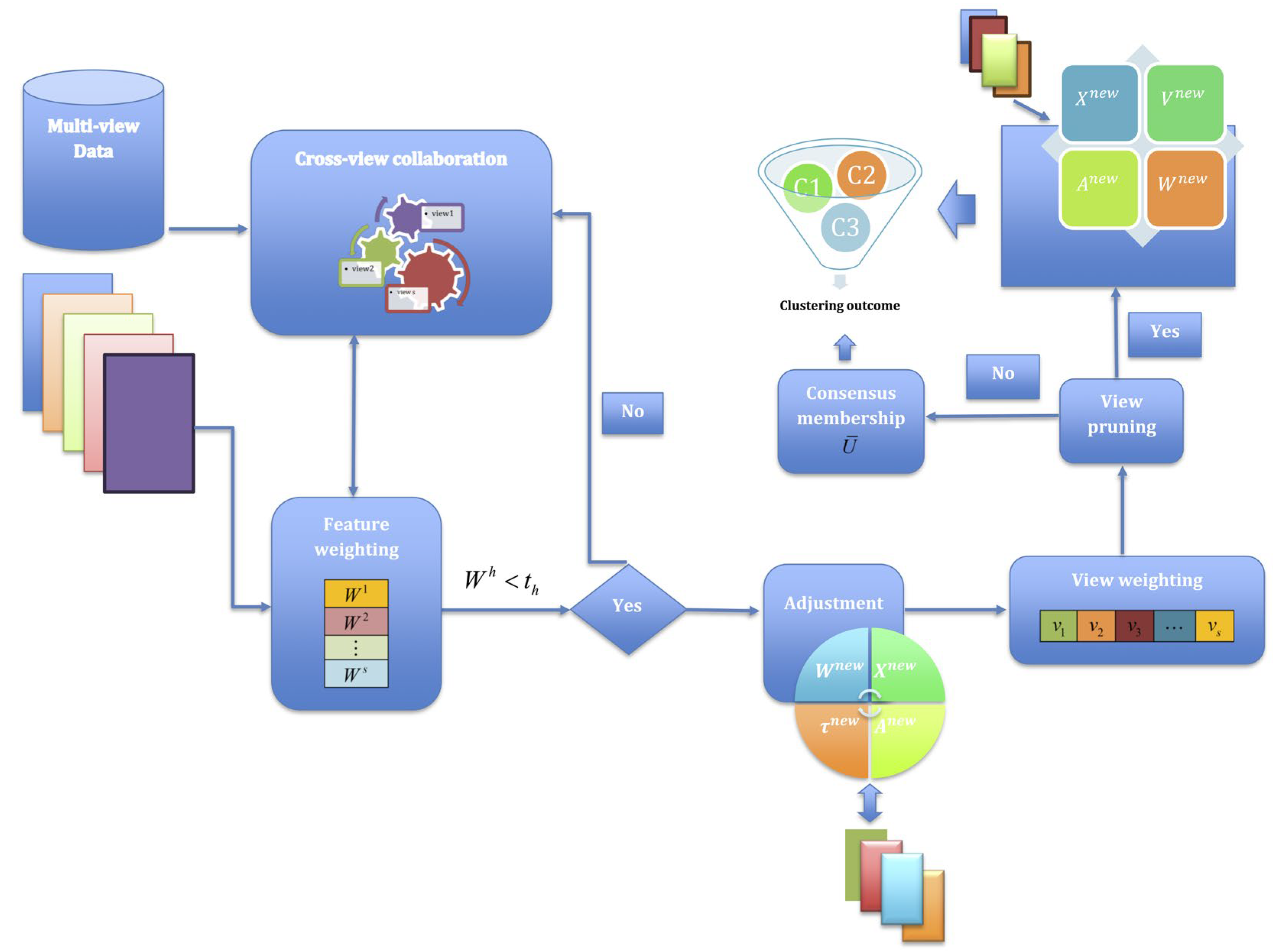Figure 1 illustrates the overall architecture of the G-CoMVKM algorithm, illustrating the flow from multi-view data input through feature weighting, cross-view collaboration, and feature pruning to final clustering output.

As shown in Figure 1, the algorithm begins with multi-view input data, where each view may contain different feature representations of the same entities. These features undergo an adaptive weighting process that determines their importance for clustering. Simultaneously, membership information is shared across views through a collaborative learning mechanism that transfers knowledge between views. The algorithm then employs a feature-pruning process that automatically identifies and eliminates redundant or irrelevant features using a threshold-based approach. Unlike feature pruning which occurs automatically, view pruning in G-CoMVKM is an optional user-guided process. The algorithm computes weights for each view, but the decision to exclude views with minimal weights depends on empirical validation. We recommend that users evaluate clustering performance both with and without the lowest-weighted views. If excluding a low-weight view improves clustering accuracy, we suggest discarding that view from the global solution. This empirical approach to view selection ensures optimal performance while maintaining interpretability. The entire integrated process iterates until convergence, producing the final clustering result with optimized feature-view weights. Most existing weighted MVKM algorithms can distinguish between relevant and weakly relevant features, but they cannot effectively eliminate redundant, unimportant, or noisy features [23,24,25,26]. In contrast, G-CoMVKM enables all relevant components across views to enhance collaborative learning while automatically pruning irrelevant features.

3.2. Problem Formulation and Objective Function

In this subsection, we formulate the G-CoMVKM objective function, which integrates adaptive feature weighting, cross-view collaborative learning, and automatic feature pruning mechanisms. Before diving into the mathematical formulation, we first provide an intuitive explanation of our approach. The core idea of G-CoMVKM is to perform clustering by balancing three key objectives including distance minimization, cross-view knowledge transfer, and feature pruning. Distance minimization aims to minimize the weighted distance between data points and their assigned cluster centers across views. Cross-view knowledge facilitates information sharing between different views through a collaborative transfer learning mechanism. Feature pruning is designed to automatically identify and eliminate irrelevant or redundant features using a threshold-based approach.

The mathematical formulation of G-CoMVKM is designed to address the challenges of clustering high-dimensional multi-view data by integrating feature-view reduction and collaborative learning. Unlike traditional MVKM methods, G-CoMVKM balances local view importance and global consensus, resulting in improved scalability, interpretability, and clustering accuracy. Most existing weighted MVKM algorithms can distinguish between relevant and weakly relevant features but are unable to effectively remove redundant, uninformative, or noisy features [25,26,27,29]. To overcome this limitation, we propose G-CoMVKM, which enables collaborative learning across all relevant components from multiple views. The objective function of G-CoMVKM is formulated as follows:

$$J_{G\text{-}CoMVKM}={\displaystyle \sum _{h=1}^s{\left(v_h\right)}^{\gamma }}\left({\displaystyle \sum _{k=1}^c{\displaystyle \sum _{i=1}^n{\mu }_{ik}^h{\displaystyle \sum _{j=1}^{d_h}{w}_j^h{\tau }_j^h{d}_{ik}^h+\delta \rho }}}\right)+\theta {\displaystyle \sum _{h=1}^s{\displaystyle \sum _{j=1}^{d_h}{w}_j^h\log }}({\tau }_j^h{w}_j^h)$$

(1)

where $\rho ={\displaystyle \sum _{\begin{array}{l}{h}^{\prime }=1,\\ h^{\prime }\ne h\end{array}}^s\left({\displaystyle \sum _{k=1}^c{\displaystyle \sum _{i=1}^n\left|{\mu }_{ik}^{h^{\prime }}-{\mu }_{ik}^h\right|\left({\displaystyle \sum _{j=1}^{d_h}{w}_j^h{\tau }_j^h{d}_{ik}^h-{\displaystyle \sum _{j=1}^{d_{h^{\prime }}}{w}_j^{h^{\prime }}{\tau }_j^{h^{\prime }}{d}_{ik}^{h^{\prime }}}}\right)}}\right)} , d_{ik}^h={\left(x_{ij}^h-a_{kj}^h\right)}^2$ and ${\displaystyle {\sum }_{h=1}^s{\displaystyle {\sum }_{k=1}^c{\mu }_{ik}^h=1,}}$ ${\mu }_{ik}^h\in \left\{0,1\right\}$, ${\displaystyle {\sum }_{h=1}^s{v}_h=1}, v_h\in \left[0,1\right],$ and ${\displaystyle {\sum }_{j=1}^{d_h}{w}_j^h}=1, w_j^h\in \left[0,1\right]$.

3.3. Component-Wise Explanation of the Objective Function

As can be seen in Equation (1), the objective function of our proposed G-CoMVKM consists of two main components including collaborative clustering term in the first term and entropy-regularized feature-view reduction in the second term. The first term promotes clustering within each view while encouraging collaboration across views throughout the $\rho$ term. This enables the algorithm to leverage complementary information and achieve a global consensus. The second term, weighted by $\theta$, is an entropy regularization that encourages sparsity in feature weights. This term penalizes uninformative or redundant features, allowing the algorithm to dynamically eliminate them based on a threshold criterion. Features with small weights are considered unimportant and are pruned, resulting in effective dimensionality reduction.

To provide a clearer understanding, we explain each component of the objective function:

$${\displaystyle \sum _{h=1}^s{\left(v_h\right)}^{\gamma }}{\displaystyle \sum _{k=1}^c{\displaystyle \sum _{i=1}^n{\mu }_{ik}^h}}{\displaystyle \sum _{j=1}^{d_h}{w}_j^h{\tau }_j^h}{(x_{ij}^h-a_{kj}^h)}^2$$

(2)

The term presented in Equation (2) performs weighted k-means clustering across all views. The weights $v_h$ and $w_j^h$ determine the importance of each view and feature, respectively. The exponent $\gamma$ and penalty parameter ${\tau }_j^h$ control the distribution of these weights. A larger $\gamma$ increases the view weight disparity, allowing dominant views to have more influence. Similarly, a larger ${\tau }_j^h$ enhances the feature weight discrimination.

$$\delta {\displaystyle \sum _{h=1}^s{\displaystyle \sum _{\begin{array}{l}{h}^{\prime }=1,\\ h^{\prime }\ne h\end{array}}^s{\displaystyle \sum _{k=1}^c{\displaystyle \sum _{i=1}^n\left|{\mu }_{ik}^{h^{\prime }}-{\mu }_{ik}^h\right|}}}}\left({\left(v_h\right)}^{\gamma }{\displaystyle \sum _{j=1}^{d_h}{w}_j^h{\tau }_j^h}{(x_{ij}^h-a_{kj}^h)}^2-{\left(v_{h^{\prime }}\right)}^{\gamma }{\displaystyle \sum _{j=1}^{d_{h^{\prime }}}{w}_j^{h^{\prime }}{\tau }_j^{h^{\prime }}}{(x_{ij}^{h^{\prime }}-a_{kj}^{h^{\prime }})}^2\right)$$

(3)

As displayed in Equation (3), this term facilitates G-CoMVKM cross-view knowledge transfer by minimizing the disagreement between weighted distances across different views. The parameter $\delta$ controls the strength of this collaboration. A larger $\delta$ enforces stronger agreement between views, promoting consistency in the clustering results. For more details, we provide a brief description of implementation transfer learning through three key mechanisms. The 1st key is cross-view disagreement quantification. The expression $\left|{\mu }_{ik}^{h^{\prime }}-{\mu }_{ik}^h\right|$ measures the disagreement in cluster assignments between views h and h′ for each data point i. When views disagree on cluster assignments, this term captures potentially complementary information. The 2nd key is distance-based knowledge transfer. The term ${\displaystyle \sum _{j=1}^{d_h}{w}_j^h}{\tau }_j^h{d}_{ik}^h-{\displaystyle \sum _{j=1}^{d_{h^{\prime }}}{w}_j^{h^{\prime }}}{\tau }_j^{h^{\prime }}{d}_{ik}^{h^{\prime }}$ compares weighted distances across views, facilitating the transfer of structural information from one view to another. This allows G-CoMVKM to leverage complementary clustering structures that may be more prominent in certain views. While the 3rd key is adaptive transfer strength. The parameter $\delta$ in Equation (1) controls the strength of knowledge transfer between views. A larger value of $\delta$ enforces stronger collaboration, while a smaller value preserves more view-specific information.

$$\theta {\displaystyle \sum _{h=1}^s{\displaystyle \sum _{j=1}^{d_h}{w}_j^h\log }}({\tau }_j^h{w}_j^h)$$

(4)

In Equation (4), entropy-based terms prevent the algorithm from assigning extreme weights to specific views or features. They ensure a more balanced weight distribution while still allowing the algorithm to identify and prioritize the most informative components.

$$w_j^h<t_h,\hspace{1em}\forall h=1,\dots ,s,\hspace{1em}\forall j=1,\dots ,d_h$$

(5)

During optimization, features with weights below a predefined threshold $t_h$ are excluded from further computation. This mechanism ensures that only informative features and views contribute to the clustering process, improving both accuracy and computational efficiency. This constraint in Equation (5) implements the feature pruning mechanism by setting feature weights below a certain threshold $t_h$ to zero. This effectively eliminates irrelevant or redundant features from the clustering process, improving both performance and interpretability. The threshold $t_h$ plays a crucial role in the feature pruning mechanism. It determines which features are considered relevant for clustering. In our implementation, $t_h$ is adaptively set based on the distribution of feature weights within each view. In our scenario, the threshold estimator ($t_h$) includes $1/n, 1/D, t/\sqrt{nD}, s/\sqrt{nD}, t/n{d}_h$, and ${\theta /\left(\sqrt{n{d}_h}\right)}^{-1}$. In summary, our threshold represents the division of the actual number of iterations, the total number of dimensionalities of s views input data, the total number of data points, and the number of dimensionalities within one data view. This adaptive threshold allows the algorithm to automatically determine the appropriate level of sparsity for each view.

3.4. Optimization

Theorem 1.

The necessary and sufficient conditions for minimizing the objective function $J_{G\text{-}CoMVKM}$ in Equation (1) with respect to cluster memberships ${\mu }_{ik}^h$, cluster centers $a_{kj}^h$, view weights $v_h$, and feature weights $w_j^h$ are given as follows:

$${\mu }_{ik}^h=\left\{\begin{array}{c}1 \mathrm{if} k=\arg \underset{1\le q\le c}{\min }{\left(v_h\right)}^{\gamma }{\zeta }^h-\delta n{\left(v_h\right)}^{\gamma }\left({\zeta }^h-{\displaystyle {\sum }_{\begin{array}{l}{h}^{\prime }=1,\\ h^{\prime }\ne h\end{array}}^s\zeta h^{\prime }}\right)\hfill \\ 0, \mathrm{Otherwise}\hfill \end{array}\right.$$

(6)

$$a_{kj}^h={\displaystyle \frac{{\displaystyle \sum _{i=1}^n{\mu }_{ik}^h{\mathsf{\Theta }}_j^h}+\delta {\displaystyle \sum _{\begin{array}{l}{h}^{\prime }=1,\\ h^{\prime }\ne h\end{array}}^s{\displaystyle \sum _{i=1}^n\left|{\mu }_{ik}^{h^{\prime }}-{\mu }_{ik}^h\right|{\mathsf{\Theta }}_j^h}}}{{\displaystyle \sum _{i=1}^n{\mu }_{ik}^h{\mathsf{\Theta }}_j^h}+\delta {\displaystyle \sum _{\begin{array}{l}{h}^{\prime }=1,\\ h^{\prime }\ne h\end{array}}^s{\displaystyle \sum _{i=1}^n\left|{\mu }_{ik}^{h^{\prime }}-{\mu }_{ik}^h\right|{\mathsf{\Theta }}_j^h}}}}{x}_{ij}^h$$

(7)

$$v_h={\left({\displaystyle \frac{{\displaystyle \sum _{r=1}^s\gamma \left({\displaystyle \sum _{k=1}^c{\displaystyle \sum _{i=1}^n{\mu }_{ik}^r{\zeta }^r+\delta \rho }}\right)}}{\gamma \left({\displaystyle \sum _{k=1}^c{\displaystyle \sum _{i=1}^n{\mu }_{ik}^h{\zeta }^h+\delta \rho }}\right)}}\right)}^{{\displaystyle \frac{1}{\gamma -1}}}$$

(8)

$$w_j^h={\displaystyle \frac{\frac{1}{{\tau }_j^h}\exp \left(-{\varpi }_h\left({\displaystyle \sum _{k=1}^c{\displaystyle \sum _{i=1}^n{\mu }_{ik}^h}}{\tau }_j^h{d}_{ik}^h+\delta {\rho }^{\prime }\right)\right)}{{\displaystyle \sum _{j^{\prime }=1}^{d_h}\frac{1}{{\tau }_{j^{\prime }}^h}\exp \left(-{\varpi }_h\left({\displaystyle \sum _{k=1}^c{\displaystyle \sum _{i=1}^n{\mu }_{ik}^h}}{\tau }_{j^{\prime }}^h{d}_{ik}^h+\delta {\rho }^{\prime }\right)\right)}}}$$

(9)

where $\rho ={\displaystyle \sum _{\begin{array}{l}{h}^{\prime }=1,\\ h^{\prime }\ne h\end{array}}^s\left({\displaystyle \sum _{k=1}^c{\displaystyle \sum _{i=1}^n\left|{\mu }_{ik}^{h^{\prime }}-{\mu }_{ik}^h\right|\left({\displaystyle \sum _{j=1}^{d_h}{w}_j^h{\tau }_j^h{d}_{ik}^h-{\displaystyle \sum _{j=1}^{d_{h^{\prime }}}{w}_j^{h^{\prime }}{\tau }_j^{h^{\prime }}{d}_{ik}^{h^{\prime }}}}\right)}}\right)} , d_{ik}^h={\left(x_{ij}^h-a_{kj}^h\right)}^2$and${\mathsf{\Theta }}_j^h=w_j^h{\tau }_j^h$.

Proof. 

The necessary condition to minimize $J_{G\text{-}Co\text{-}MVKM}$ w.r.t. ${\mu }_{ik}^h$ is similar to the k-means, and so the updating equation for ${\mu }_{ik}^h$ can be obtained with Equation (6). To find the necessary condition to minimize $J_{G\text{-}Co\text{-}MVKM}$ w.r.t. $a_{kj}^h$, we need to differentiate $J_{G\text{-}CoMVKM}$ w.r.t. $a_{kj}^h$ by treating other variables as fixed. First, we differentiate $\rho$ w.r.t. $a_{kj}^h$ with ${\displaystyle \frac{\partial \rho }{\partial a_{kj}^h}}={\displaystyle \frac{\partial }{\partial a_{kj}^h}}\left(\left({\displaystyle \sum _{\begin{array}{l}{h}^{\prime }=1,\\ h^{\prime }\ne h\end{array}}^s\left({\displaystyle \sum _{k=1}^c{\displaystyle \sum _{i=1}^n\left|{\mu }_{ik}^{h^{\prime }}-{\mu }_{ik}^h\right|\left({\displaystyle \sum _{j=1}^{d_h}{w}_j^h{\tau }_j^h{d}_{ik}^h-{\displaystyle \sum _{j=1}^{d_{h^{\prime }}}{w}_j^{h^{\prime }}{\tau }_j^{h^{\prime }}{d}_{ik}^{h^{\prime }}}}\right)}}\right)} \right)\right)=0.$ Then, we get ${\displaystyle \frac{\partial \rho }{\partial a_{kj}^h}}={\displaystyle \frac{\partial }{\partial a_{kj}^h}}\left(\left({\displaystyle \sum _{\begin{array}{l}{h}^{\prime }=1,\\ h^{\prime }\ne h\end{array}}^s{\displaystyle \sum _{k=1}^c{\displaystyle \sum _{i=1}^n\left|{\mu }_{ik}^{h^{\prime }}-{\mu }_{ik}^h\right|\left({\displaystyle \sum _{j=1}^{d_h}{w}_j^h{\tau }_j^h{\left(x_{ij}^h-a_{kj}^h\right)}^2}\right)}}} \right)\right)=0.$ Due to $-{\displaystyle \sum _{\begin{array}{l}{h}^{\prime }=1,\\ h^{\prime }\ne h\end{array}}^s{\displaystyle \sum _{i=1}^n\left|{\mu }_{ik}^{h^{\prime }}-{\mu }_{ik}^h\right|w_j^h{\tau }_j^h}}\left(x_{ij}^h-a_{kj}^h\right)=0$, and let ${\mathsf{\Theta }}_j^h=w_j^h{\tau }_j^h$, we have $\mathsf{\Omega }={\displaystyle \frac{\partial J_{G\text{-}Co\text{-}MVKM}}{\partial a_{kj}^h}}=-{\displaystyle \sum _{\begin{array}{l}{h}^{\prime }=1,\\ h^{\prime }\ne h\end{array}}^s{\displaystyle \sum _{i=1}^n\left|{\mu }_{ik}^{h^{\prime }}-{\mu }_{ik}^h\right|{\mathsf{\Theta }}_j^h}}\left(x_{ij}^h-a_{kj}^h\right)=0.$ Thus, we obtain ${\displaystyle \frac{\partial J_{G-CoFLKM}}{\partial a_{kj}^h}}={\left(v_h\right)}^{\gamma }\left(-{\displaystyle \sum _{i=1}^n{\mu }_{ik}^h{\mathsf{\Theta }}_j^h\left(x_{ij}^h-a_{kj}^h\right)+\delta \mathsf{\Omega }}\right)=0$ and ${\left(v_h\right)}^{\gamma }\left(-{\displaystyle \sum _{i=1}^n{\mu }_{ik}^h{\mathsf{\Theta }}_j^h\left(x_{ij}^h-a_{kj}^h\right)-\delta {\displaystyle \sum _{\begin{array}{l}{h}^{\prime }=1,\\ h^{\prime }\ne h\end{array}}^s{\displaystyle \sum _{i=1}^n\left|{\mu }_{ik}^{h^{\prime }}-{\mu }_{ik}^h\right|{\mathsf{\Theta }}_j^h}}\left(x_{ij}^h-a_{kj}^h\right)}\right)=0.$ They can convert to $-{\displaystyle \sum _{i=1}^n{\mu }_{ik}^h{\mathsf{\Theta }}_j^h{x}_{ij}^h+{\displaystyle \sum _{i=1}^n{\mu }_{ik}^h{\mathsf{\Theta }}_j^h{a}_{kj}^h}-\delta {\displaystyle \sum _{\begin{array}{l}{h}^{\prime }=1,\\ h^{\prime }\ne h\end{array}}^s{\displaystyle \sum _{i=1}^n\left|{\mu }_{ik}^{h^{\prime }}-{\mu }_{ik}^h\right|{\mathsf{\Theta }}_j^h{x}_{ij}^h+}}\delta {\displaystyle \sum _{\begin{array}{l}{h}^{\prime }=1,\\ h^{\prime }\ne h\end{array}}^s{\displaystyle \sum _{i=1}^n\left|{\mu }_{ik}^{h^{\prime }}-{\mu }_{ik}^h\right|{\mathsf{\Theta }}_j^h{a}_{kj}^h}}}=0.$ We note that ${\displaystyle \sum _{i=1}^n{\mu }_{ik}^h{\mathsf{\Theta }}_j^h{a}_{kj}^h}+\delta {\displaystyle \sum _{\begin{array}{l}{h}^{\prime }=1,\\ h^{\prime }\ne h\end{array}}^s{\displaystyle \sum _{i=1}^n\left|{\mu }_{ik}^{h^{\prime }}-{\mu }_{ik}^h\right|{\mathsf{\Theta }}_j^h{a}_{kj}^h}}={\displaystyle \sum _{i=1}^n{\mu }_{ik}^h{\mathsf{\Theta }}_j^h{x}_{ij}^h}+\delta {\displaystyle \sum _{\begin{array}{l}{h}^{\prime }=1,\\ h^{\prime }\ne h\end{array}}^s{\displaystyle \sum _{i=1}^n\left|{\mu }_{ik}^{h^{\prime }}-{\mu }_{ik}^h\right|{\mathsf{\Theta }}_j^h{x}_{ij}^h}}$ and $\left({\displaystyle \sum _{i=1}^n{\mu }_{ik}^h{\mathsf{\Theta }}_j^h}+\delta {\displaystyle \sum _{\begin{array}{l}{h}^{\prime }=1,\\ h^{\prime }\ne h\end{array}}^s{\displaystyle \sum _{i=1}^n\left|{\mu }_{ik}^{h^{\prime }}-{\mu }_{ik}^h\right|{\mathsf{\Theta }}_j^h}}\right)a_{kj}^h=\left({\displaystyle \sum _{i=1}^n{\mu }_{ik}^h{\mathsf{\Theta }}_j^h}+\delta {\displaystyle \sum _{\begin{array}{l}{h}^{\prime }=1,\\ h^{\prime }\ne h\end{array}}^s{\displaystyle \sum _{i=1}^n\left|{\mu }_{ik}^{h^{\prime }}-{\mu }_{ik}^h\right|{\mathsf{\Theta }}_j^h}}\right)x_{ij}^h$. Therefore, the updated equation of $J_{G\text{-}Co\text{-}MVKM}$ w.r.t. $a_{kj}^h$ is obtained as Equation (7). To find the necessary condition to minimize $J_{G\text{-}Co\text{-}MVKM}$ w.r.t. $v_h$, we can treat all other variables as constants and differentiate w.r.t. $v_h$. The terms that do not depend on $v_h$ will disappear, $J_{G\text{-}Co\text{-}MVKM}$ will be left with $J_{G\text{-}Co\text{-}MVKM}={\displaystyle \sum _{h=1}^s{\left(v_h\right)}^{\gamma }}\left({\displaystyle \sum _{k=1}^c{\displaystyle \sum _{i=1}^n{\mu }_{ik}^h{\displaystyle \sum _{j=1}^{d_h}{w}_j^h{\tau }_j^h{d}_{ik}^h+\delta \rho }}}\right)$. The Lagrangian of $J_{G\text{-}Co\text{-}MVKM}$ corresponding to $v_h$ can be expressed as ${\tilde{J}}_{G\text{-}Co\text{-}MVKM}=J_{G\text{-}Co\text{-}MVKM}+{\lambda }_2\left({\displaystyle \sum _{h=1}^s{v}_h-1}\right)$. To take the derivative of ${\tilde{J}}_{G\text{-}Co\text{-}MVKM}$ w.r.t. $v_h$, we have that ${\displaystyle \frac{\partial {\tilde{J}}_{G\text{-}Co\text{-}MVKM}}{\partial v_h}}={\displaystyle \frac{\partial }{\partial v_h}}\left(J_{G\text{-}CoFLKM}+{\lambda }_2\left({\displaystyle \sum _{h=1}^s{v}_h-1}\right)\right)=0$, and then both $\gamma {\left(v_h\right)}^{\gamma -1}\left({\displaystyle \sum _{k=1}^c{\displaystyle \sum _{i=1}^n{\mu }_{ik}^h{\displaystyle \sum _{j=1}^{d_h}{w}_j^h{\tau }_j^h{d}_{ik}^h+\delta \rho }}}\right)+{\lambda }_2=0$ and ${\left(v_h\right)}^{\gamma -1}=-{\lambda }_2/\gamma \left({\displaystyle \sum _{k=1}^c{\displaystyle \sum _{i=1}^n{\mu }_{ik}^h{\zeta }^h+\delta \rho }}\right)$ are obtained. They can be reformulated as $v_h={\left(-{\lambda }_2/\gamma \left({\displaystyle \sum _{k=1}^c{\displaystyle \sum _{i=1}^n{\mu }_{ik}^h{\zeta }^h+\delta \rho }}\right)\right)}^{{\displaystyle \frac{1}{\gamma -1}}}$. Since ${\displaystyle \sum _{h=1}^s{v}_h-1=0}$, we have ${\displaystyle \sum _{r=1}^s{\left(-{\lambda }_2/\gamma \left({\displaystyle \sum _{k=1}^c{\displaystyle \sum _{i=1}^n{\mu }_{ik}^h{\zeta }^h+\delta \rho }}\right)\right)}^{\frac{1}{\gamma -1}}}-1=0$ and ${\displaystyle \sum _{r=1}^s{\left(\gamma \left({\displaystyle \sum _{k=1}^c{\displaystyle \sum _{i=1}^n{\mu }_{ik}^r{\zeta }^r+\delta \rho }}\right)\right)}^{-1}}={\left(-{\lambda }_2\right)}^{-1}$, and then ${\displaystyle \sum _{r=1}^s\gamma \left({\displaystyle \sum _{k=1}^c{\displaystyle \sum _{i=1}^n{\mu }_{ik}^r{\zeta }^r+\delta \rho }}\right)}=-{\lambda }_2$. Thus, we have the update equation for $v_h$ as $v_h={\left({\displaystyle \sum _{r=1}^s\gamma \left({\displaystyle \sum _{k=1}^c{\displaystyle \sum _{i=1}^n{\mu }_{ik}^r{\zeta }^r+\delta \rho }}\right)}/\gamma \left({\displaystyle \sum _{k=1}^c{\displaystyle \sum _{i=1}^n{\mu }_{ik}^h{\zeta }^h+\delta \rho }}\right)\right)}^{{\displaystyle \frac{1}{\gamma -1}}}$. To find the partial derivative of $J_{G\text{-}Co\text{-}MVKM}$ w.r.t. $w_j^h$, we need to consider the terms that depend on $w_j^h$, and differentiate them while treating all other variables as constant. To identify the relevant terms, we need to break down the objective function $J_{G\text{-}Co\text{-}MVKM}$ by removing the absolute value of ${\mu }_{ik}^{h^{\prime }}-{\mu }_{ik}^h$. The Lagrangian of $J_{G\text{-}Co\text{-}MVKM}$ corresponding to $w_j^h$ can be expressed as ${\tilde{J}}_{G\text{-}Co\text{-}MVKM}=J_{G\text{-}Co\text{-}MVKM}+{\lambda }_1\left({\displaystyle \sum _{j=1}^{d_h}{w}_j^h-1}\right)$. First, we have that ${\displaystyle \frac{\partial \rho }{\partial w_j^h}}={\displaystyle \sum _{\begin{array}{l}{h}^{\prime }=1,\\ h^{\prime }\ne h\end{array}}^s\left({\displaystyle \sum _{k=1}^c{\displaystyle \sum _{i=1}^n\left|{\mu }_{ik}^{h^{\prime }}-{\mu }_{ik}^h\right|{\tau }_j^h{d}_{ik}^h}}\right)}={\displaystyle \sum _{k=1}^c{\displaystyle \sum _{i=1}^n\left({\displaystyle \sum _{\begin{array}{l}{h}^{\prime }=1,\\ h^{\prime }\ne h\end{array}}^s\left|{\mu }_{ik}^{h^{\prime }}-{\mu }_{ik}^h\right|}\right){\tau }_j^h{d}_{ik}^h}}$. Therefore, to simplify the notation, we write ${\rho }^{\prime }=\partial \rho /\partial w_j^h={\displaystyle \sum _{k=1}^c{\displaystyle \sum _{i=1}^n\left({\displaystyle \sum _{\begin{array}{l}{h}^{\prime }=1,\\ h^{\prime }\ne h\end{array}}^s{\mu }_{ik}^{h^{\prime }}-{\mu }_{ik}^h}\right){\tau }_j^h{d}_{ik}^h}}$. The partial derivation of ${\tilde{J}}_{G\text{-}Co\text{-}MVKM}$ w.r.t. $w_j^h$ can be represented as ${\displaystyle \frac{\partial {\tilde{J}}_{G\text{-}Co\text{-}MVKM}}{\partial w_j^h}}={\displaystyle \frac{\partial \left({\displaystyle \sum _{h=1}^s{\left(v_h\right)}^{\gamma }}\left({\displaystyle \sum _{k=1}^c{\displaystyle \sum _{i=1}^n{\mu }_{ik}^h{\displaystyle \sum _{j=1}^{d_h}{w}_j^h{\tau }_j^h{d}_{ik}^h+\delta \rho }}}\right)+\theta {\displaystyle \sum _{h=1}^s{\displaystyle \sum _{j=1}^{d_h}{w}_j^h\log }}{\tau }_j^h{w}_j^h+{\lambda }_1\left({\displaystyle \sum _{j=1}^{d_h}{w}_j^h-1}\right)\right)}{\partial w_j^h}}=0$. Then ${\left(v_h\right)}^{\gamma }\left({\displaystyle \sum _{k=1}^c{\displaystyle \sum _{i=1}^n{\mu }_{ik}^h}}{\tau }_j^h{d}_{ik}^h+\delta {\rho }^{\prime }\right)+\theta \left(\log {\tau }_j^h{w}_j^h+1\right)+{\lambda }_1=0$ can be easily converted as $\log {\tau }_j^h{w}_j^h={\displaystyle \frac{-{\left(v_h\right)}^{\gamma }\left({\displaystyle \sum _{k=1}^c{\displaystyle \sum _{i=1}^n{\mu }_{ik}^h}}{\tau }_j^h{d}_{ik}^h+\delta {\rho }^{\prime }\right)-{\lambda }_1}{\theta }}-1$. Similarly, let $\log {\tau }_j^h{w}_j^h={\displaystyle \frac{-{\left(v_h\right)}^{\gamma }\left({\displaystyle \sum _{k=1}^c{\displaystyle \sum _{i=1}^n{\mu }_{ik}^h}}{\tau }_j^h{d}_{ik}^h+\delta {\rho }^{\prime }\right)}{\theta }}-\left({\displaystyle \frac{{\lambda }_1}{\theta }}+1\right)$ be converted to ${\tau }_j^h{w}_j^h=\exp \left({\displaystyle \frac{-{\left(v_h\right)}^{\gamma }\left({\displaystyle \sum _{k=1}^c{\displaystyle \sum _{i=1}^n{\mu }_{ik}^h}}{\tau }_j^h{d}_{ik}^h+\delta {\rho }^{\prime }\right)}{\theta }}\right)/\exp \left({\displaystyle \frac{{\lambda }_1}{\theta }}+1\right)$. Therefore, we have that $w_j^h={\displaystyle \frac{1}{{\tau }_j^h}}\exp \left({\displaystyle \frac{-{\left(v_h\right)}^{\gamma }\left({\displaystyle \sum _{k=1}^c{\displaystyle \sum _{i=1}^n{\mu }_{ik}^h}}{\tau }_j^h{d}_{ik}^h+\delta {\rho }^{\prime }\right)}{\theta }}\right)/\exp \left({\displaystyle \frac{{\lambda }_1}{\theta }}+1\right)$ and $w_j^h={\displaystyle \frac{\frac{1}{{\tau }_j^h}\exp \left(-{\varpi }_h\left({\displaystyle \sum _{k=1}^c{\displaystyle \sum _{i=1}^n{\mu }_{ik}^h}}{\tau }_j^h{d}_{ik}^h+\delta {\rho }^{\prime }\right)\right)}{{\displaystyle \sum _{j^{\prime }=1}^{d_h}\frac{1}{{\tau }_{j^{\prime }}^h}\exp \left(-{\varpi }_h\left({\displaystyle \sum _{k=1}^c{\displaystyle \sum _{i=1}^n{\mu }_{ik}^h}}{\tau }_{j^{\prime }}^h{d}_{ik}^h+\delta {\rho }^{\prime }\right)\right)}}}$ (*). Since ${\displaystyle \sum _{j=1}^{d_h}{w}_j^h-1=0}$, we obtain that ${\displaystyle \sum _{j^{\prime }=1}^{d_h}\frac{1}{{\tau }_{j^{\prime }}^h}\exp \left(\frac{-{\left(v_h\right)}^{\gamma }\left({\displaystyle \sum _{k=1}^c{\displaystyle \sum _{i=1}^n{\mu }_{ik}^h}}{\tau }_{j^{\prime }}^h{d}_{ik}^h+\delta {\rho }^{\prime }\right)}{\theta }\right)=\exp \left(\frac{{\lambda }_1}{\theta }+1\right)}$ (**). By substituting (**) into (*), we have $w_j^h={\displaystyle \frac{1}{{\tau }_j^h}}\exp \left({\displaystyle \frac{-{\left(v_h\right)}^{\gamma }\left({\displaystyle \sum _{k=1}^c{\displaystyle \sum _{i=1}^n{\mu }_{ik}^h}}{\tau }_j^h{d}_{ik}^h+\delta {\rho }^{\prime }\right)}{\theta }}\right)/{\displaystyle \sum _{j^{\prime }=1}^{d_h}\frac{1}{{\tau }_{j^{\prime }}^h}\exp \left(\frac{-{\left(v_h\right)}^{\gamma }\left({\displaystyle \sum _{k=1}^c{\displaystyle \sum _{i=1}^n{\mu }_{ik}^h}}{\tau }_{j^{\prime }}^h{d}_{ik}^h+\delta {\rho }^{\prime }\right)}{\theta }\right)}$. Now let ${\varpi }_h={\left(v_h\right)}^{\gamma }/\theta$, then the updated equation for feature weight $w_j^h$ can be expressed as $w_j^h={\displaystyle \frac{\frac{1}{{\tau }_j^h}\exp \left(-{\varpi }_h\left({\displaystyle \sum _{k=1}^c{\displaystyle \sum _{i=1}^n{\mu }_{ik}^h}}{\tau }_j^h{d}_{ik}^h+\delta {\rho }^{\prime }\right)\right)}{{\displaystyle \sum _{j^{\prime }=1}^{d_h}\frac{1}{{\tau }_{j^{\prime }}^h}\exp \left(-{\varpi }_h\left({\displaystyle \sum _{k=1}^c{\displaystyle \sum _{i=1}^n{\mu }_{ik}^h}}{\tau }_{j^{\prime }}^h{d}_{ik}^h+\delta {\rho }^{\prime }\right)\right)}}}$. This is Equation (9). □

3.5. Parameter, Threshold Setting and Impact

In addition to excluding irrelevant features within a single view of multiple representation data commonly known as MV data, we are experimenting with G-CoMVKM with a scheme of decreasing the number of views using feature-view-weighted based G-CoMVKM. The purpose of this experiment is to discover specific insights within one view during clustering processes. The idea is simply to answer whether there is a nonzero effect or not if we exclude unlikely or even unrealistic views during computation. Views with lower contributions are considered less important and can be excluded from the clustering process, thereby reducing the computational complexity, and improving the clustering performance. By combining both feature-level and view-level selection criteria in a collaborative manner, G-CoMVKM can effectively handle high-dimensional MV datasets by transforming them into lower dimensionalities using a subset reduction framework of redundant or noisy features. The feature-level selection helps to identify relevant features of each view, while the view-level selection helps to identify unlikely or even unrealistic views during the clustering process. Together, they help to improve the accuracy and efficiency of the clustering process of the proposed G-CoMVKM.

There are four essential parameters in the proposed G-CoMVKM an exponent parameter $\gamma$ to handle the distribution of one data view, a balancing parameter $\delta$ to handle the disagreement across views, a balancing parameter $\theta$ to regularize the entropy weights to lead to feature pruning, and a penalty parameter $\tau$ to handle the distribution of feature-view components. We need to define $\gamma$ as well as possible to be matched for a collaboration step. Since multi-view data is varied, the measurement to control each data view h is also different from each other. Generally, we specify $\gamma$ as a user defines with $\gamma \in \left[3,\infty \right]$. In G-CoMVKM, the parameter $\theta$ is also user-defined, with $\theta \in \left[0,1\right]$, for producing a desirable result, the starting point is 0.1 with incremental step 0.05 or 0.1. For producing a proper lower number of dimensionalities within one view on some MV data, tuning the parameter $\theta$ with criterion $\theta >2$ and $\gamma \in \left[0,1\right]$ are recommended. Detailed analysis of these two parameters of $\gamma$ and $\theta$ will be given in the experiments and results section. The estimation for ${\tau }_j^h$ depends on the minimum, mean, and maximum input data within one view, formulated as below:

$${\tau }_j^h=\mathrm{mean}\left({\displaystyle \frac{x_{ij}^h}{{\displaystyle {\sum }_{i=1}^n{x}_{ij}^h}}}\right)/\mathrm{mean}\left(\underset{i}{\max }{x}_{ij}^h-\underset{i}{\min }{x}_{ij}^h\right)$$

(10)

As visualized in Equation (10), the mean of data view measures the dispersion of feature weights and mean of maximization/minimum of data points in each view guaranteeing the variation of data sets. To exclude irrelevant features within one view during clustering processes, we need to take a threshold into account. We discontinue unimportant features-view by using some selection threshold criteria. In our scenario, the threshold estimator $\left(t_h\right)$ including $1/n, 1/D, t/\sqrt{nD}, s/\sqrt{nD}, t/n{d}_h,$ and ${\theta /\left(\sqrt{n{d}_h}\right)}^{-1}$. In our procedure, we define $\delta =\gamma \theta$, a multiplication between parameters to handle the distribution of view weights, and regularization for feature weights work better to handle collaborative transfer learning in our proposed G-CoMVKM. This adaptive balancing parameter maintains the greater weight variance, impacting clearer discrimination between important and unimportant features.

3.6. Fusion Stage

The initial memberships are randomly generated and updated based on the input data within one view taking advantage of its own local and collaborative steps weighting component. In the very first stage, different views will have different membership values. The updating equation of view weight, cluster centers, and feature weights is then calculated in their own loop, locally. In this sense, we can name it as a local updating estimation. Each feature-view component within multi-view data interacted with each other based on its weights to transform the original dimension of MV data into a new lower dimensionality without matrices-based reconstruction approaches. In the scenario, it simply transfers their information to build an agreement for generating a global solution considering feature based-threshold reduction step. As our global solution is formulated, a new transformation of original MV data expectedly will have lower dimensions containing relevant feature component. The global solution will be finally made by integrating the membership of the local step, named a fusion step. This fusion step will conclude the final pattern of multi-view data. Our fusion step is formulated as follows.

$$\overline{U}={\displaystyle \sum _{h=1}^s{\mu }_{ik}^h{v}_h}$$

(11)

where ${\mu }_{ik}^h$ is the membership of ith data point assigned in the kth cluster for hth view, and $v_h$ is the weight for the hth view.

3.7. Algorithm Implementation

In this subsection, we outline the full implementation of the proposed G-CoMVKM clustering algorithm (Algorithm 1). The algorithm begins by initializing the cluster centers, feature weights, and view weights, and then, it iteratively updates these variables until convergence or until the maximum number of iterations is reached. Thus, the proposed G-CoMVKM algorithm is summarized as follows in which Figure 2 demonstrates its flowchart.

Algorithm 1. The G-CoMVKM Clustering Algorithm

Input: Multi-view dataset $X=\left\{x_1,x_2,\dots ,x_n\right\}$ with $x_i={\left\{x_i^h\right\}}_{h=1}^s,x_i^h={\left\{x_{ij}^h\right\}}_{j=1}^{d_h}$, number of clusters c, parameters $\gamma ,\delta ,\theta$, maximum iterations t, convergence threshold $ϵ$ Initialization: Initialize cluster centers $a_{kj}^h$ randomly or using k-means++ Initialize feature weights $w_j^h=1/d_h$ for all $j=1,\dots ,d_h,h=1,\dots ,s$ Initialize view weights $v_h=1/s$ for all $h=1,\dots ,s$ $t=0$ and $J_{G\text{-}CoMVKM}^{\left(0\right)}=\infty$ While $t<t_{\max }$ and $\left|J_{G\text{-}CoMVKM}^{\left(t\right)}-J_{G\text{-}CoMVKM}^{\left(t-1\right)}\right|>ϵ$ do       // Compute penalty parameter       Compute ${\tau }_j^h$ by Equation (10).       // Compute membership matrix       for $i=1$ to $n$ do              for $k=1$ to $c$ do                       Calculate $D_{ik}={\left(v_h\right)}^{\gamma }{\displaystyle \sum _{j=1}^{d_h}{w}_j^h{\tau }_j^h}{(x_{ij}^h-a_{kj}^h)}^2-{\left(v_{h^{\prime }}\right)}^{\gamma }{\displaystyle \sum _{j=1}^{d_{h^{\prime }}}{w}_j^{h^{\prime }}{\tau }_j^{h^{\prime }}}{(x_{ij}^{h^{\prime }}-a_{kj}^{h^{\prime }})}^2$                       Compute ${\mu }_{ik}^h$ according to Equation (6)       // Update Cluster Centers       for $h=1$ to $s$ do              for $k=1$ to $c$ do                     for $j=1$ to $d_h$ do                       Calculate ${\mathsf{\Theta }}_j^h$                       Compute $a_{kj}^h$ according to Equation (7)       // Update Feature Weights       for $h=1$ to $s$ do              for $j=1$ to $d_h$ do                       Calculate $\rho ={\displaystyle \sum _{h^{\prime }=1,h^{\prime }\ne h}^s\left({\displaystyle \sum _{k=1}^c{\displaystyle \sum _{i=1}^n\left|{\mu }_{ik}^{h^{\prime }}-{\mu }_{ik}^h\right|}}\left({\displaystyle \sum _{j=1}^{d_h}{w}_j^h}{\tau }_j^h{d}_{ik}^h-{\displaystyle \sum _{j=1}^{d_{h^{\prime }}}{w}_j^{h^{\prime }}}{\tau }_j^{h^{\prime }}{d}_{ik}^{h^{\prime }}\right)\right)}$                       Update $w_j^h$ according to Equation (9)       // Feature pruning       for $h=1$ to $s$ do              Calculate threshold $t_h$              for $j=1$ to $d_h$ do                       set $w_j^h=0$ if $w_j^h<t_h$              Renormalize remaining non-zero weights: $w_j^h=w_j^h/{\displaystyle {\sum }_{j^{\prime }=1}^{d_h}{w}_{j^{\prime }}^h}$       // Update viee weights       for $h=1$ to $s$ do              Calculate ${\zeta }^h$              Update $v_h$ according to Equation (8)       // View pruning             for $h=1$ to $s$ do              set $v_h=0$ if $v_h=\min \left(v_h\right)$              Renormalize remaining non-zero weights: $v_h=v_h/{\displaystyle {\sum }_{r=1}^s{v}_r}$       // Calculate objective function value       Calculate $J_{G\text{-}CoMVKM}^{\left(t+1\right)}$ according to Equation (1)       $t=t+1$

3.8. Computational Complexity and Initialization Sensitivity

The computational complexity of G-CoMVKM is an important consideration, especially when dealing with large-scale multi-view datasets. As a non-convex optimization problem, G-CoMVKM employs Lagrangian multiplier techniques to derive the update functions for each variable while satisfying the respective constraints. This analytical approach, while mathematically elegant, inherits the initialization sensitivity common to many clustering algorithms in the k-means family. Similar to k-means and its variants, G-CoMVKM’s convergence to a global optimum cannot be guaranteed due to the non-convex nature of its objective function. The algorithm typically converges to a local minimum, with the quality of this solution being heavily dependent on the initial cluster centers, feature weights, and view weights. Multiple runs with different initializations are often necessary to identify a robust solution—a common practice in non-convex clustering frameworks.

With these considerations in mind, we analyze the complexity of each major step in the algorithm, accounting for both the computational requirements and the iterative nature needed to mitigate initialization sensitivity. First, for the membership updating of ${\mu }_{ik}^h$, we need to compute the distance to each cluster center across all views. The computational complexity is $O(n\times c\times s\times \overline{d})$, where n is the number of samples, c is the number of clusters, s is the number of views, and $\overline{d}={\displaystyle \frac{1}{s}}{\displaystyle \sum _{h=1}^s{d}_h}$ is the average dimensionality across views. Second, for the cluster center updating of $a_{kj}^h$, it requires computing the weighted sum of all assigned samples, and so the computational complexity is $O(n\times c\times s\times \overline{d})$. Third, for the view weight updating of $v_h$, it involves computing memberships and cluster centers and so has a complexity of $O(n\times c\times s\times \overline{d})$. Similarly, for feature weight updating of $w_j^h$, it has a complexity of $O(n\times c\times s\times \overline{d})$. Thus, the overall computational complexity of the G-CoMVKM algorithm should be $O(n\times c\times s\times \overline{d}\times t)$, where t is the number of iterations.

3.9. Comparison with Existing Methods

Table 2. Computational Complexity Comparison.

Algorithm	Time Complexity	Space Complexity
TW-K-means	$O(n\times c\times s\times \overline{d}\times t)$	$O(n\times c\times s\times \overline{d})$
WMCFS	$O(n\times c\times s\times \overline{d}\times t)$	$O(n\times c\times s\times \overline{d})$
SWVF	$O(n\times c\times s\times \overline{d}\times t)$	$O(n\times c\times s\times \overline{d})$
TW-Co-K-means	$O(n\times c\times s^2\times \overline{d}\times t)$	$O(n\times c\times s^2\times \overline{d})$
FRMVK	$O(n\times c\times s\times \overline{d}\times t)$	$O(n\times c\times s\times \overline{d})$
G-CoMVKM	$O(n\times c\times s\times \overline{d}\times t)$	$O(n\times c\times s\times \overline{d})$

compares the computational complexity of G-CoMVKM with existing multi-view clustering algorithms.

Despite incorporating the collaborative transfer mechanism and feature pruning, G-CoMVKM maintains the same asymptotic complexity as basic multi-view k-means variants like TW-K-means and FRMVK. This is achieved through efficient implementation of the updating rules and pruning mechanism. The computational advantage becomes even more significant as the algorithm progresses because feature pruning reduces the effective dimensionality with each iteration, view weights concentrate on the most informative views, allowing for potential view-based early stopping strategies, and adaptive threshold calculation adds negligible overhead. In practice, G-CoMVKM shows superior computational efficiency compared to TW-Co-K-means due to the latter’s quadratic dependency on the number of views. Additionally, G-CoMVKM’s feature pruning mechanism not only improves interpretability but also enhances computational efficiency by reducing the effective dimensionality during clustering.

4. Experiments and Results

In this section, numerical and real data sets will be implemented to evaluate the performances of the proposed G-CoMVKM and several related MVKM algorithms.

Table 3. Experiments with the numerical data set before and after withdrawing irrelevant features.

	V1D2C		V2D3C			AR
	${\mathit{x}}_1^1$	${\mathit{x}}_2^1$	${\mathit{x}}_1^2$	${\mathit{x}}_2^2$	${\mathit{x}}_3^2$
Initials	0.5	0.5	0.333	0.333	0.333
Iteration 0	0.483	0.517	0.382	0.480	0.138	0.362
Iteration 1	0.483	0.517	0.443	0.557	Dropped out	0.362
Iteration 2	0.483	0.517	0.443	0.557		0.344
Iteration 3	0.483	0.517	0.443	0.557		1.00
Iteration 4	0.483	0.517	0.443	0.557		1.00

summarizes detailed information of ten real-world applications and

Table 4. Experiments with the numerical data set before and after withdrawing irrelevant features.

	View Weights		${\mathit{\mu }}_{\mathit{k}}^1$		${\mathit{\mu }}_{\mathit{k}}^2$		$\overline{\mathit{U}}$
	V1D2C	V2D3C	C1	C2	C1	C2	C1	C2
Initials	0.5	0.5	-	-	-	-	-	-
Iteration 0	0.487	0.513	371	629	653	347	515.8	484.2
Iteration 1	0.474	0.527	371	629	653	347	519.6	480.5
Iteration 2	0.497	0.503	572	428	615	385	593.6	406.4
Iteration 3	0.493	0.507	533	467	533	467	533	467
Iteration 4	0.494	0.507	533	467	533	467	533	467

summarizes detailed parameter settings of related methods used as comparisons. All algorithms in our experiments are evaluated by using three evaluation clustering metrics: accuracy rate (AR), Rand Index (RI) [35], and Normalized Mutual Information (NMI) [36,37]. The AR is calculated by using ${\displaystyle {\sum }_{k=1}^c{n}_k/n}$ where n is the number of data points and $n_k$ is the number of correctly clustered data points in cluster k. The RI evaluates how similar the cluster assignments are to one another by making pair-wise comparisons. Let $\left(P_i,P_j\right)$ be a given pair of points from the data set. Let $a$ be the number of pairs of points in which both points belong to the same cluster in $C$ and the same cluster in $C^{\prime }$, b denote the number of point pairs in which both points belong to two different clusters $C$ and two different clusters in $C^{\prime }$, $c$ be the number of pairs of points if the two points belong to the same cluster in $C$ and different clusters in $C^{\prime }$, and $d$ be the number of pairs of points if the two points belong to two different clusters in $C$ and to the same cluster in $C^{\prime }.$ The overall number $M=n\left(n-1\right)/2$ of possible point pairs within the dataset and the number n of data points are used to determine RI with $RI=\left(a+d\right)/M$. NMI measures the amount of information on the presence/absence of a term that contributes to making the correct classification decision [36,37]. NMI is computed by $\mathrm{NMI}=MI\left(y,\hat{y}\right)/\left([H\left(y\right)+H\left(\hat{y}\right)]/2\right)$, where $H\left(y\right)$ and $H\left(\hat{y}\right)$ are the marginal entropies of $y$ and $\hat{y}$, respectively, and $MI\left(y,\hat{y}\right)$ is a mutual information between the ground truth $y$ and the predicted $\hat{y}$ cluster. The values of AR, RI, and NMI range from 0 to 1. Thus, a higher value indicates larger similarity. The worst value is close to 0, and the best value is close to 1.

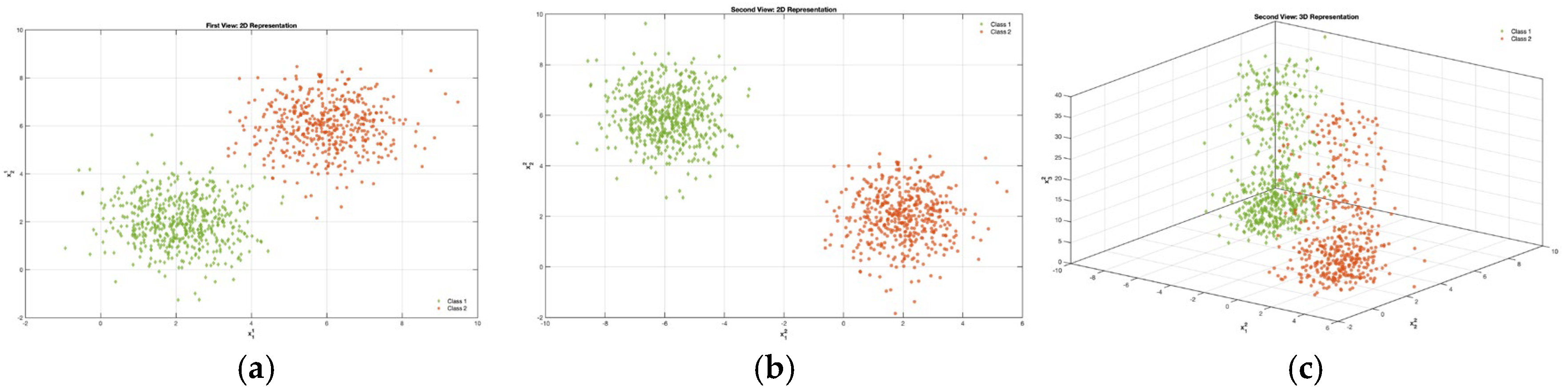
Example 1.

A two-dimensional two-view data with 1000 points distributed into two clusters is generated from a 2-component 2-variate Gaussian mixture model (GMM), as shown in Figure 3a–c, is called 2V2D2C. View 1 is named as V1D2C, while view 2 is named V2D3C. These $x_1^1$ and $x_2^1$ are the coordinates for V1D2C, while $x_1^2$, $x_2^2$, and $x_3^2$ are the coordinates for V2D3C. The means ${\mu }_k^1$ for V1D2C in the 2V2D2C data are $\left(2,2\right)$ and $\left(6,6\right)$. The means ${\mu }_k^2$ for V2D3C in the 2V2D2C data are $\left(-6,6\right)$ and $\left(2,2\right)$. The covariance matrices and mixing proportions for the two views are ${\displaystyle {\sum }_1^1={\displaystyle {\sum }_2^1={\displaystyle {\sum }_1^2={\displaystyle {\sum }_2^2=\left(\begin{array}{cc}1& 0\\ 0& 1\end{array}\right)}}}}$, ${\alpha }_k^1={\alpha }_k^2=1/2, k=1,2$, respectively. To simulate our scenario in selecting relevant features with automatically unimportant feature-reduction, an additional feature component $x_3^2$ is added to V3D2C. We design all feature components in view 1 that are relevant, thus the procedure of reduction is expected to not be applied and continuously processed as they retain as good features. The additional feature is generated from a uniform distribution to demonstrate unimportant features within one view in this multi-view data scenario, with the range from 50 to 60. In this experiment, we investigate the ability of our proposed G-CoMVKM algorithm to detect the unimportant features within each data view.

Table 3 shows the results of our experiments on this syntactic data by dropping out unimportant features during the clustering processes. As can be seen in Table 3, the proposed G-CoMVKM effectively shows its ability to correctly measure the quality of feature-view components and views. It can identify the third component of V2D3C as a non-informative feature and automatically exclude it from the account after iteration 1. While the remaining feature-view components of V1D2C handle the robustness to improve the accuracy by 65.6% after the third iteration. The experimental results successfully support our hypothesis to find a good pattern by exploiting the relevancy of both feature and view components subjected to reduce the dimensionality of each view that is designed as a noisy-feature-view. Moreover, the distribution of data points within one cluster for a single view (locally) and globally across views is reported in Table 4. As shown in Table 4, G-CoMVKM converges completely after 4 iterations, with view weights distribution stabilizing by the 3rd iteration. This stable distribution of weights determines the final assignment of data points across clusters. The early stabilization of some weights, far from being problematic, demonstrates the algorithm’s efficiency in identifying and preserving important features while focusing computational effort on optimizing features that require more refinement.

Example 2.

In this experiment, we consider two real datasets, called Wikipedia Articles [38] and Prokaryotic phyla [39]. The detailed information of these two datasets is displayed in Table 5. The purpose of this experiment is to learn a typical threshold for filtering the unimportant noisy or redundant features within one view. Our experiments will include some learning thresholds to see the effect of dimensionality reduction in advance. Our learning threshold will use the current number of dimensionality, number of data points, number of iterations, and number of views to distinguish a pair of essential feature-view components from a pair of unimportant feature-view components. This behavior occurs because:

• Feature importance stability: These features ($x_1^1,x_2^1$ for view 1 and $x_1^2,x_2^2$ for view 2) represent highly informative dimensions that are immediately recognized by the algorithm as significant for clustering. Their weights stabilize early because they consistently provide strong discriminative power.
• View-specific convergence: Different views may converge at different rates depending on their information content. In this case, the stable weights indicate that the algorithm quickly identified the optimal weighting for these specific features.
• Collaborative learning effect: The collaborative learning mechanism in G-CoMVKM can accelerate convergence for features that have strong consensus across views, resulting in early stabilization of their weights.

Table 5. A Summary of Seven Real World Datasets.

Data Sets	Characteristics
	# of h	# of n	# of c	Name of Views	# of d
Biological data
Prokaryotic phyla [39]	3	551	4	Gene repertoire	393
				Proteome composition	3
				Textual	438
Image data
MNIST4 [40]	3	4000	4	ISO	30
				LDA	9
				NPE	30
COIL20 [41]	3	1440	20	Degree $\left[0^{\circ },{85}^{\circ }\right]$	30
				Degree $\left[{90}^{\circ },{175}^{\circ }\right]$	19
				Degree $\left[{180}^{\circ },{265}^{\circ }\right]$	30
ORL Face [42]	4	400	40	Intensity	4096
				LBP	3304
				Gabor	6750
				PHOG	1024
Text and Image Data
Wikipedia articles [38]	2	639	10	Text	128
				Image	10
Motion or Human Activity Recognition (HAR) Data
DHA [43]	2	253	23	RGB view	6144
				Depth view	110
UWA [44]	2	254	30	RGB view	6144
				Depth view	110

Table 5. A Summary of Seven Real World Datasets.

Data Sets	Characteristics
	# of h	# of n	# of c	Name of Views	# of d
Biological data
Prokaryotic phyla [39]	3	551	4	Gene repertoire	393
				Proteome composition	3
				Textual	438
Image data
MNIST4 [40]	3	4000	4	ISO	30
				LDA	9
				NPE	30
COIL20 [41]	3	1440	20	Degree $\left[0^{\circ },{85}^{\circ }\right]$	30
				Degree $\left[{90}^{\circ },{175}^{\circ }\right]$	19
				Degree $\left[{180}^{\circ },{265}^{\circ }\right]$	30
ORL Face [42]	4	400	40	Intensity	4096
				LBP	3304
				Gabor	6750
				PHOG	1024
Text and Image Data
Wikipedia articles [38]	2	639	10	Text	128
				Image	10
Motion or Human Activity Recognition (HAR) Data
DHA [43]	2	253	23	RGB view	6144
				Depth view	110
UWA [44]	2	254	30	RGB view	6144
				Depth view	110

As comparisons, we employ TW-k-means, WMCFS, SWVF, TW-Co-k-means, and FRMVK to quantify the superiority of our proposed G-CoMVKM. Note that the parameter settings on these five competitive algorithms of TW-k-means, WMCFS, SWVF, TW-Co-k-means, and FRMVK are presented in

Table 6. Parameter Setting of Six Related Algorithms.

Data Sets	TW-k-Means	WMCFS	SWVF	TW-Co-k-Means	FRMVK	G-CoMVKM
Prokaryotic Phyla	$\begin{array}{l}\eta =10,\\ \beta =5\end{array}$	$\alpha =7,\beta =5\times {10}^{-3}$	$\alpha =5,\beta =4$	$\begin{array}{l}\alpha =60,\beta =50,\\ \eta =0.45\end{array}$	$\alpha =8$	$\gamma =3,\theta =4$
Coil20		$\alpha =7,\beta =5\times {10}^{-3}$	$\alpha =5,\beta =4\times {10}^{-4}$	$\begin{array}{l}\alpha =6,\beta =5,\\ \eta =0.45\end{array}$		$\gamma =0.5,\theta =8$
MNIST4		$\alpha =7,\beta =5\times {10}^{-6}$
ORL Face		$\alpha =57\times {10}^{-7},\beta =8$	$\alpha =8,\beta =25\times {10}^{-4}$	$\begin{array}{l}\alpha =35,\beta =7,\\ \eta =0.25\end{array}$		$\gamma =0.35,\theta =8$
Wikipedia Articles	$\begin{array}{l}\eta =10,\\ \beta =5\end{array}$	$\alpha =10,\beta =25\times {10}^{-2}$	$\alpha =5,\beta =4$	$\begin{array}{l}\alpha =60,\beta =50,\\ \eta =0.45\end{array}$	$\alpha =8$	$\gamma =0.35,\theta =6$
DHA		$\alpha =57\times {10}^{-7},\beta =8$	$\alpha =8,\beta =25\times {10}^{-4}$		$\alpha =4$	$\gamma =0.7,\theta =8$
UWA		$\alpha =3\times {10}^{-6},\beta =8$	$\alpha =8,\beta =45\times {10}^{-4}$	$\begin{array}{l}\alpha =60,\beta =50,\\ \eta =0.45\end{array}$	$\alpha =5$	$\gamma =0.95,\theta =20$

.

The behavior of different thresholds on Wikipedia articles data produced by G-CoMVKM are displayed in

Table 7. The Clustering Performances of G-CoMVKM On Wikipedia Articles Data under Different Thresholds.

Thresholds	${\mathit{v}}_{\mathit{h}}$		$\mathbf{Final} {\mathit{d}}_{\mathit{h}}$		$\overline{\mathit{U}}$	Clustering Performances
	Text View	Image View	${\mathit{d}}_1$	${\mathit{d}}_2$		AR	RI	NMI
$t/\sqrt{nD}$	0.515	0.482	8	8	[107; 31; 43; 57; 57; 86; 139; 44; 70; 59]	0.470	0.869	0.482
$s/\sqrt{nD}$	0.514	0.486	30	10	[68; 101; 84; 57; 73; 50; 67; 65; 80; 48]	0.552	0.885	0.536
$1/n$	0.512	0.488	121	10	[104; 57; 86; 24; 33; 76; 74; 71; 113; 55]	0.547	0.885	0.541
$1/D$	0.515	0.485	13	10	[57; 69; 87; 58; 78; 62; 67; 109; 44; 62]	0.561 *	0.886 *	0.542 *

* Bold face indicates the best one, _ indicates the second best one.

. As can be seen, the first view of Wikipedia Articles, which is represented by text data, shows a trend of dimensionality reduction. The highest performance was obtained when the remaining dimension of the text view is 13, producing 56.13% ARs, 88.55% RIs, and 54.15% NMIs. Here, the image feature-view components are consistently relevant when these thresholds of $s/\sqrt{nD}, 1/n,$ and $1/D$ assigned to exclude the unimportant feature from the account. In Prokaryotic Phyla data, the best performance is reached when threshold $t_h=t/\sqrt{nD}$, displayed in

Table 8. The Clustering Performances of G-CoMVKM On Prokaryotic Data Set under Different Thresholds.

Thresholds	${\mathit{v}}_{\mathit{h}}$			$\mathbf{Final} {\mathit{d}}_{\mathit{h}}$			$\overline{\mathit{U}}$	Clustering Performances
	Gene Repertoire	Proteome Composition	Textual	${\mathit{d}}_1$	${\mathit{d}}_2$	${\mathit{d}}_3$		AR	RI	NMI
$t/\sqrt{nD}$	0.317	0.329	0.354	4	3	7	[140.1; 103.8; 53.1; 59.3]	0.623 *	0.676 *	0.406 *
$s/\sqrt{nD}$	0.285	0.357	0.358	4	3	3	[50.9; 97.6; 91.4; 114.1]	0.582	0.664	0.384
$1/n$	0.297	0.340	0.363	375	3	371	[107.5; 113.5; 74.4; 55.1]	0.561	0.642	0.318
$1/D$	0.299	0.335	0.367	393	3	438	[115.9; 75.1; 54.5; 103.6]	0.570	0.644	0.317

* Bold face indicates the best one, _ indicates the second best one.

. The three feature-view components are reduced to 4, 3, and 7, respectively. To be noted, the maximum iterations in this experiment were set manually and each experiment ran under 100 different random initializations. The performances of five related algorithms on Wikipedia articles [38] and prokaryotic phyla data [39] are reported in

Table 9. Experimental Results for Wikipedia Articles and Prokaryotic Data Sets.

Evaluation Criteria	Wikipedia Articles			Prokaryotic
	AR	RI	NMI	AR	RI	NMI
TW-k-means	0.527	0.879	0.539	0.294	0.522	0.006
WMCFS	0.425	0.629	0.361	0.553	0.645	0.325
SWVF	0.523	0.877	0.544 *	0.442	0.582	0.157
TW-Co-k-means	0.554	0.885	0.540	0.521	0.594	0.235
FRMVK	0.555	0.881	0.530	0.561	0.644	0.323
G-CoMVKM	0.561 *	0.886 *	0.542	0.625 *	0.676 *	0.406 *

* Bold face indicates the best one, _ indicates the second best one.

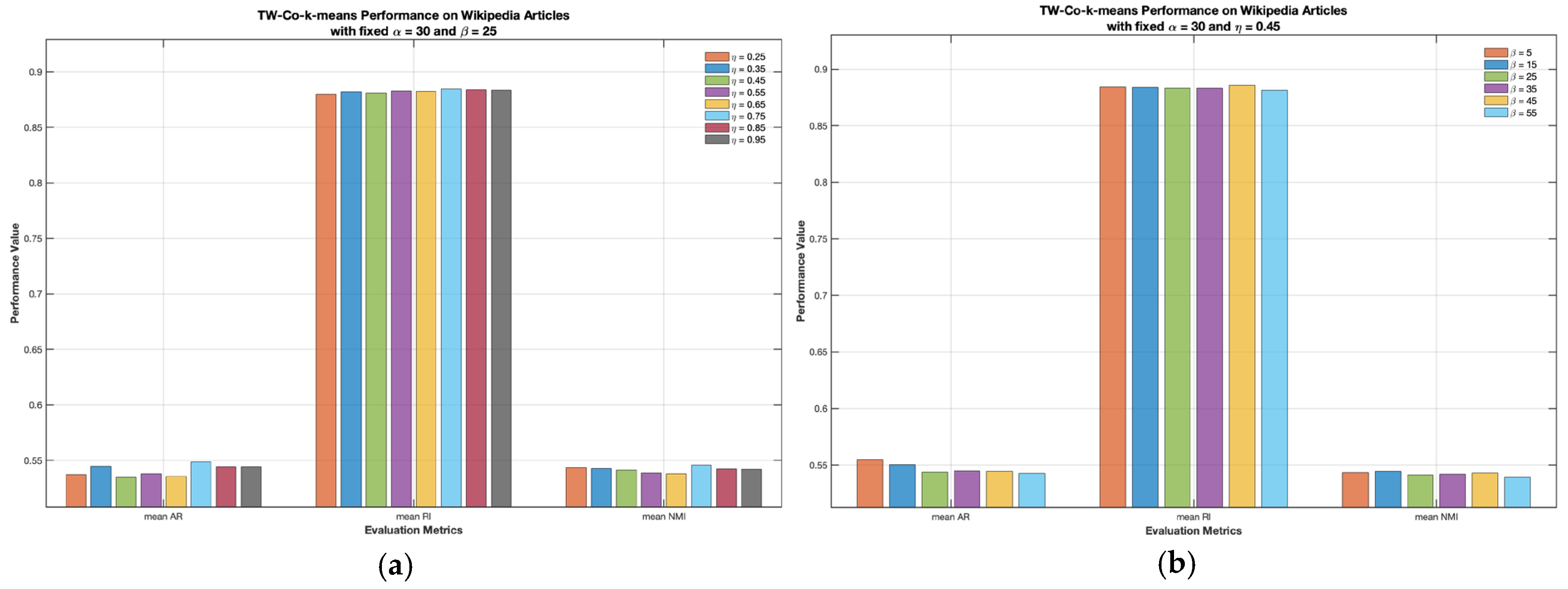
. As can be seen in Table 7, the proposed G-CoMVKM performs better as compared to these six related methods with 56.13% Ars, 88.55% Ars, and 54.15% NMIs on Wikipedia articles: 62.49% ARs, 67.57% RIs, and 40.60% NMIs on Prokaryotic phyla data. Using this example, we investigate the impact of parameters $\eta$, $\alpha$, and $\beta$ of TW-Co-k-means clustering algorithm on the Wikipedia articles data set. As can be seen in Figure 4a,b, given by the certain value of the fixed parameter and different values of another parameter of TW-Co-k-means on Wikipedia articles does not significantly affect the clustering performances. The final dimensionalities after feature reductions on Wikipedia articles and Prokaryotic Phyla performed by our proposed G-CoMVKM and FRMVK clustering algorithms are reported in

Table 10. Summary of Relevant Features By FRMVK and G-CoMVKM on Wikipedia Articles and Prokaryotic Data Sets.

Evaluation Criteria	Wikipedia Articles		Prokaryotic
	Text	Image	Gene Repertoire	Proteome Composition	Textual
FRMVK	57	10	116	3	124
G-CoMVKM	13	10	4	3	7

. As shown in Table 10, compared to FRMVK with final $d_h=\left[\begin{array}{cc}57& 10\end{array}\right]$ on Wikipedia articles and $d_h=\left[\begin{array}{ccc}116& 3& 124\end{array}\right]$ on prokaryotic phyla. Our proposed G-CoMVKM final $d_h=\left[\begin{array}{cc}13& 10\end{array}\right]$ on Wikipedia articles performs better with an improvement about 0.63% ARs, 0.51% RIs, and 1.15% NMIs. While final $d_h=\left[\begin{array}{ccc}4& 3& 7\end{array}\right]$ on prokaryotic phyla makes an improvement about 6.35% ARs, 3.14% RIs, and 8.31% NMIs.

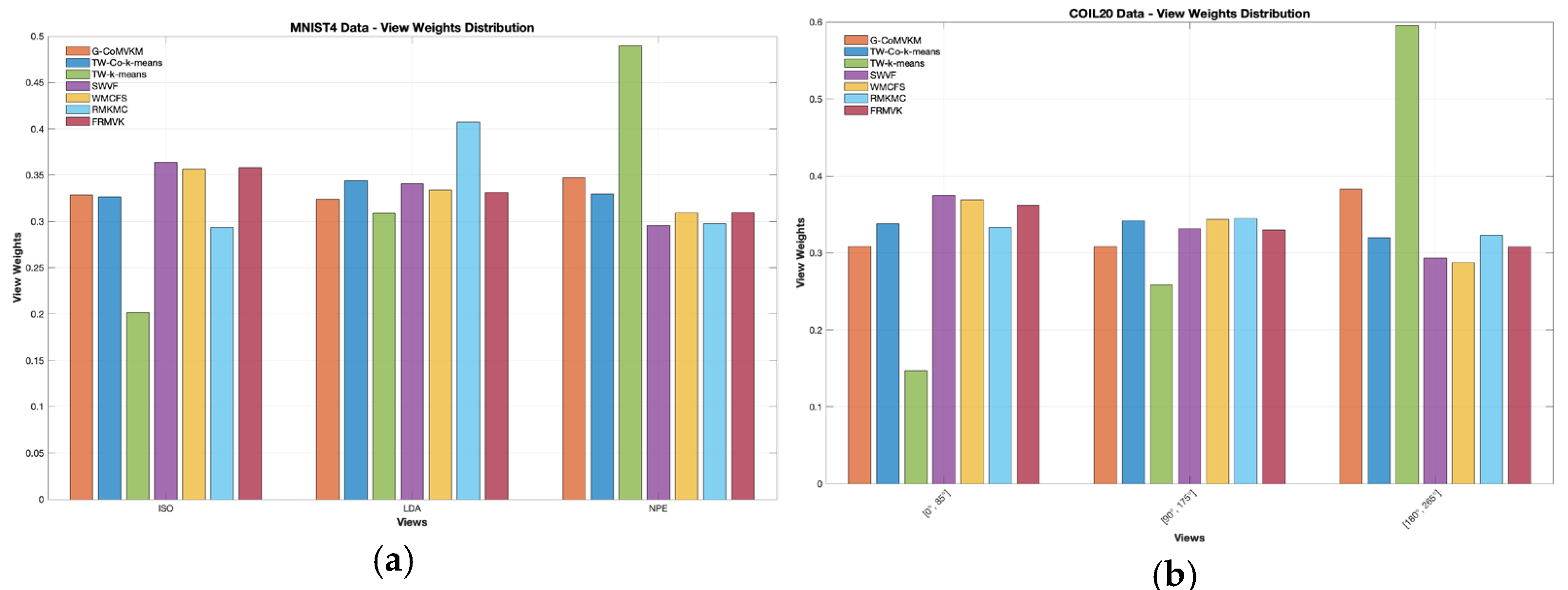
Example 3.

In this experiment, real-world applications such as COIL20 [41] and MNIST [40] datasets, will be used to see the effectiveness of the proposed G-CoMVKM in demonstrating data with larger sizes of data points and clusters. The detailed information of these data is reported in Table 5. For simulation purposes, all the algorithms are set to be run manually and using the default parameter setting provided in Table 6. Additionally, we set up the maximum number of iterations for each running algorithm as 35 times and report the minimum, average, and maximum values based on a hundred simulations.

Table 11. The Clustering Performances (Minimum, Mean, and Maximum AR, RI, NMI) and Total Running Time (TRT) of Each Employed Competitive Algorithms and Proposed G-CoMVKM on COIL20 Data Set.

	AR	RI	NMI	TRT
TW-k-means	0.565/0.631/0.701	0.511/0.589/0.655	0.767/0.854/0.902	6032.7
WMCFS	0.236/0.382/0.562	0.198/0.357/0.546	0.222/0.401/0.606	6176.3
SWVF	0.476/0.561/0.679	0.357/0.487/0.633	0.636/0.747/0.866	6177.7
TW-Co-k-means	0.535/0.613/0.680	0.484/0.566/0.654	0.701/0.793/0.872	2818.6
FRMVK	0.716 */0.752 */0.781	0.707/0.743/0.776	0.880 */0.902 */0.919 *	394.0
G-CoMVKM	0.579/0.719/0.798 *	0.947 */0.967 */0.976 *	0.815/0.867/0.889	34.50 *

* Bold face indicates the best one, _ indicates the second best one.

and

Table 12. The Clustering Performances (Minimum, Mean, and Maximum AR, RI, NMI) and Total Running Time (TRT) of Each Employed Competitive Algorithms and Proposed G-CoMVKM on MNIST4 Data Set.

	AR	RI	NMI	TRT
TW-k-means	0.729/0.786/0.845	0.567/0.627/0.681	0.623/0.659/0.696	3001.1
WMCFS	0.801/0.816/0.820	0.576/0.587/0.592	0.566/0.575/0.578	1790.6
SWVF	0.722/0.794/0.851	0.556/0.628/0.684	0.616/0.661/0.696	3038.3
TW-Co-k-means	0.729/0.777/0.831	0.570/0.619/0.675	0.629/0.659/0.692	2608.1
FRMVK	0.804 */0.843 */0.876	0.648/0.713/0.683	0.668/0.691/0.712	571.9
G-CoMVKM	0.617/0.833/0.885 *	0.808 */0.882 */0.899 *	0.885 */0.899 */0.717 *	26.2 *

* Bold face indicates the best one, _ indicates the second best one.

reported detailed clustering performances of our proposed G-CoMVKM and five related clustering algorithms in the minimum, average, and maximum values of these ARs, RIs, and NMIs. To perform the consistency of the importance of one view within multi-view data, we employed these six competitive clustering algorithms of TW-K-means [27], WMCFS [21], SWVF [22], TW-Co-K-means [30], and FRMVK [29]. Figure 5a,b displays the distribution of view weights performed by our proposed G-CoMVKM and these six employed related clustering algorithms on MNIST4 [40], and COIL20 [41] data sets, respectively. It is clearly shown that the proposed G-CoMVKM and six employed related clustering algorithms assigned a different weight to one data view that realized its contribution during the clustering process. Based on clustering performances in Table 11 and Table 12 and data views contribution in Figure 6a,b, we next investigate the impact of parameters of WMCFS, SWVF, and FRMVK on COIL20 data shown in Figure 6a–e. As can be seen, a different number of parameters combination on WMCFS and SWVF affects the clustering performances; While FRMVK on COIL20 data perform stable when different values of parameter assigned. This analysis showed that different combination parameters must be chosen properly to enable a good clustering performance on WMCFS and SWVF. Overall, the proposed G-CoMVKM is superior as compared to five employed competitive clustering algorithms. Even in the computational cost, our proposed G-CoMVKM is considerably faster with additional feature-view weighted, collaborative, and feature reduction steps, especially on a very large number of observation data sets such as MNIST4 [40] and COIL20 [41].

Example 4.

To enhance the assessment of the proposed G-CoMVKM’s efficacy, the view importance procedures will be implemented during the clustering processes. The significance of one view will be separately evaluated using our proposed G-CoMVKM-based-feature-view-weighted approaches, which will help to exclude the bias or unrealistic view and expectedly generate more valuable insights. The approach involves selecting views with lower dimensions and analyzing them in-depth. Our focus is on examining views that offer abundant information, with particular emphasis on the features that are most pertinent for pattern recognition.

$$v_h^{\ast }=\min \left(v_1,v_2,\dots ,v_s\right)$$

(12)

The hth view with $v_h^{\ast }$ according to Equation (12) is significant and can then be subjected to a repeated process of G-CoMVKM, which excludes unimportant features to refine the results. As an experimental design to enhance accuracy, we could exclude one or two unrealistic detected views and observe if even minor changes in behavior lead to an improvement. We believe that good feature-view components can significantly boost accuracy and be more cost-effective in terms of running time. To address the effect of the decreasing number of views on MV data, we applied G-CoMVKM on Olivetti Research Laboratory (ORL) face data [42].

Table 13. The Performance of G-CoMVKM with View Dropping Out Scheme On ORL Face Data Set.

	View 1	View 2	View 3	View 4	AR	RI	NMI
ORL Face	693	1487	381	1021	0.4600 */0.5005 */0.5650 *	0.9630 */0.9682 */0.9746 *	0.7276 */0.7596 */0.7911 *
	693	1487	381	Dropped out	0.3775/0.4164/0.4500	0.9591/0.9629/0.9675	0.7072/0.7209/0.7436
	693	1487	Dropped out	996	0.3825/0.4309/0.5350	0.9626/0.9650/0.9707	0.7153/0.7290/0.7597
	693	1487	Dropped out	Dropped out	0.4025/0.4270/0.4625	0.9599/0.9632/0.9692	0.7023/0.7175/0.7483

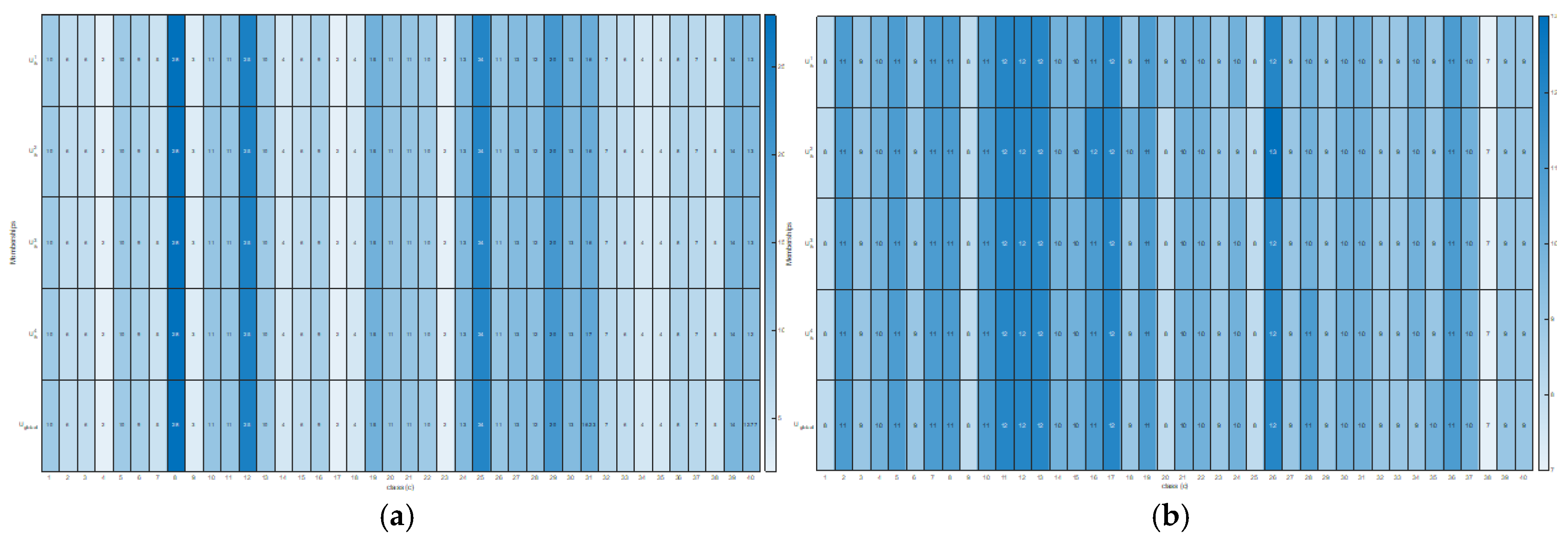
* Bold face indicates the best one, _ indicates the second best one.

reported that the G-CoMVKM produced the best results when all four view components on ORL face data were processed. It outperformed the G-CoMVKM with two or three views of ORL face as input data. In other words, there is no upgraded phenomenon when the number of views decreases. Conversely, the downgraded clustering performances happened with consistently processing all data-feature-view components obtained by G-CoMVKM on complete views. More preciously, the memberships among local and global feature-view component steps with complete views showed no tendencies of over-distributed behaviors, displayed in Figure 7a,b. Figure 8a,b displayed the feature and view weights behaviors on the ORL face data set by processing all the original view components as the input data and by decreasing the number of views, respectively. As can be seen in Figure 8a, each feature component of intensity’s, LBP’s, Gabor’s, and PHOG’s views showing trends. There exist some components with more and less contribution even after feature reduction is implemented. The high contribution of one component is occupied by the peak of the graph and the bottom indicates the lowest or less contribution. Figure 7b shows that the less the number of views, the better discriminated is the importance of one component. As the number of views decreased to two, G-CoMVKM recognized that intensity has the highest contribution in discovering the pattern of ORL face data. However, it linearly decreased the performances by 7.35% ARs, 5% RIs, and 4.21% NMIs. Observing these results, we conclude that the decreased number of views within MV data does not guarantee an upgrade phenomenon on clustering performances.

Example 5.

In this experiment, our goal is to identify motion or Human Activity Recognition (HAR) data, called UWA3D multi-view activity [43] and Depth-induced Human Action (DHA) [44]. The UWA data contains 660 action sequences; 11 actions were performed by 12 subjects with five repetitive actions. While DHA contains 483 video clips of 23 categories. These two HAR data were extracted with RGB and depth features. In this experiment, we first conduct 30 different simulations based on the G-CoMVKM algorithm and report its minimum, average, and maximum ARs, RIs, and NMIs. Secondly, we conduct an experiment by tuning the two parameters $\gamma$ and $\theta$ on UWA and DHA. Further comparisons with six related methods will be made and reported its minimum, average, and maximum clustering metric performances under 30 different simulations.

Figure 9a displays the distribution of feature components on RGB and Depth views of DHA data after feature reduction performed by G-CoMVKM. While Figure 9b displayed its view weight distributions. For DHA data, we set $\gamma$ as 0.49, 0.51, 0.59, 0.65, 0.67, and 0.69. The minimum, average, and maximum values of Ars, RIs, and NMIs produced by our proposed G-CoMVKM are displayed in a bar chart, presented in Figure 10a–c. For UWA data, we set $\gamma$ as 0.25, 0.35, 0.45, 0.55, 0.65, 0.75, 0.85, and 0.95. The minimum, average, and maximum values of its Ars, RIs, and NMIs produced by our proposed G-CoMVKM are displayed in a bar chart, presented in Figure 11a–c. The final dimensionalities of each view on DHA and UWA data after feature reduction performed by G-CoMVKM are presented in

Table 14. Final Dimensions on UWA Data After Performing G-CoFLKM with Fixed θ and Different γ.

	G-CoMVKM
	$\gamma =0.25$	$\gamma =0.35$	$\gamma =0.45$	$\gamma =0.55$	$\gamma =0.65$	$\gamma =0.75$	$\gamma =0.85$	$\gamma =0.95$
RGB	596	217	156	137	130	121	119	112
Depth	110	110	110	110	110	110	109	106

. As a comparison, the final dimensionalities produced by FRMVK are also reported in the same table. As it can be seen, all $\gamma$ produce the same final dimensionality on the Depth view when $\gamma$ is $\left[\begin{array}{cccccc}0.25& 0.35& 0.45& 0.55& 0.65& 0.75\end{array}\right]$. While it produces a different final dimensionality on both RGB and Depth views when $\gamma$ is $\left[\begin{array}{cc}0.85& 0.95\end{array}\right]$. Although all these $\gamma$ produce a different number of dimensionalities within one view, it did not affect the final clustering performances. This is due to the “relevant features” and “weakly relevant but non-redundant features” are both included and discriminated by our threshold during clustering processes. Overall, the proposed G-CoMVKM performs better as compared to another related state-of-the-art, as displayed in

Table 15. The Performance of G-CoMVKM and Five Related Algorithms On DHA and UWA Data Sets.

	HAR Data	RGB View	Depth View	Clustering Performances			TRT
				AR	RI	NMI
G-CoMVKM	DHA	147	110	0.5967 */0.6195 */0.6667*	0.9468 */0.9556 */0.9621*	0.7362 */0.7751 */0.8075*	595.728
	UWA	177		0.5415*/0.5818*/0.6245*	0.9525*/0.9618*/0.9688*	0.7610*/0.7815*/0.8086*	637.582
FRMVK	DHA	17	31	0.0658/0.1870/0.5761	0.0420/0.3127/0.9535	0.0000/0.1991/0.7121	8.781*
	UWA	1	20	0.1304/0.2694/0.4269	0.8431/0.8977/0.9430	0.3681/0.5303/0.6714	2.390*
TW-k-means	DHA	6144	110	0.3745/0.4471/0.4897	0.9266/0.9365/0.9442	0.6465/0.6673/0.7130	226.441
	UWA			0.4269/0.4900/0.5929	0.9434/0.9527/0.9610	0.6947/0.7306/0.7755	510.223
WMCFS	DHA			0.0658/0.1052/0.4691	0.0420/0.1314/0.9384	0.0000/0.0699/0.7197	223.247
	UWA			0.0553/0.0553/0.0553	0.0325/0.0325/0.0325	0.0000/0.0000/0.0000	454.559
SWVF	DHA			0.3745/0.4750/0.5432	0.9302/0.9393/0.9469	0.6416/0.6919/0.7324	233.293
	UWA			0.4704/0.5410/0.6087	0.9476/0.9596/0.9654	0.7340/0.7648/0.7914	466.964
TW-Co-k-means	DHA			0.3333/0.4016/0.4897	0.9171/0.9307/0.9405	0.6101/0.6384/0.6699	51.603
	UWA			0.4783/0.5387/0.6126	0.9512/0.9589/0.9668	0.7365/0.7638/0.7926	93.426

* Bold face indicates the best one, _ indicates the second best one.

.

5. Conclusions

In summary, the proposed G-CoMVKM algorithm can capture the local, collaborative, and global steps by taking advantage of features-view reduction into a single framework. It produces a new lower dimensionality within one view to pattern desirable MV data. While identifying redundant components and dropping them based on a threshold criterion. The G-CoMVKM succeed in transforming a new MV data with relevant feature components. Based on our experimental design and results, the proposed G-CoMVKM can process these real MV data applications and generate a feature-view reduction efficiently, without compromising on clustering performances. Overall, the G-CoMVKM is superior in terms of parameter tuning and its efficiency in transforming a high dimensionality without taking a matrices-based reconstruction approach into account. It is a simple MVKM algorithm that simultaneously enables transfer feature-view learning and feature reduction steps to form a global solution considering local and collaboration steps across data views. However, the proposed G-CoMVKM needs further improvement in terms of consideration of privacy concerns by using a concept of collaborative MV scenarios under multiple clients. Thus, our future work will consider including federated learning to discover hidden information from MV data under multiple clients.