Article

Time Series Forecasting via an Elastic Optimal Adaptive GM(1,1) Model

1
Office of Information Technology, Shandong University, Jinan 250100, China
2
School of Software, Shandong University, Jinan 250101, China
3
School of Information Science and Engineering, Shandong Normal University, Jinan 250014, China
*
Author to whom correspondence should be addressed.
Electronics 2025, 14(10), 2071; https://doi.org/10.3390/electronics14102071
Submission received: 18 April 2025 / Revised: 16 May 2025 / Accepted: 19 May 2025 / Published: 20 May 2025
(This article belongs to the Special Issue Future Technologies for Data Management, Processing and Application)

Abstract

:
The GM(1,1) model is a well-established approach for time series forecasting, demonstrating superior effectiveness with limited data and incomplete information. However, its performance often degrades in dynamic systems, leading to obvious prediction errors. To address this impediment, we propose an elastic optimal adaptive GM(1,1) model, dubbed EOAGM, to improve forecasting performance. Specifically, our proposed EOAGM dynamically optimizes the sequence length by discarding outdated data and incorporating new data, reducing the influence of irrelevant historical information. Moreover, we introduce a stationarity test mechanism to identify and adjust sequence data fluctuations, ensuring stability and robustness against volatility. Additionally, the model refines parameter optimization by incorporating predicted values into candidate sequences and assessing their impact on subsequent forecasts, particularly under conditions of data fluctuation or anomalies. Experimental evaluations across multiple real-world datasets demonstrate the superior prediction accuracy and reliability of our model compared to six baseline approaches.

1. Introduction

As a fundamental research direction in data mining [1,2], time series analysis is considered one of the top ten technical challenges of the 21st century [3,4,5]. Time series research encompasses multiple core domains, specifically including key technical directions such as time series forecasting, time series classification, time series clustering, and time series anomaly detection [6,7,8]. At its core, time series forecasting leverages historical data to uncover temporal patterns, constructing predictive models that provide quantitative foundations for trend anticipation, risk early warning, and evidence-based decision-making [9,10,11]. Research indicates that effective time series forecasting not only reveals the evolution mechanisms of systems [12,13,14] but also offers technological support for industrial upgrading, thereby facilitating the implementation of cross-industry sustainable development strategies [15,16,17].
Among various forecasting methods [18,19,20], the GM(1,1) model has garnered significant attention due to its unique capability in small-sample modeling [21,22]. As an important tool in gray system theory, this model demonstrates significant advantages in system behavior modeling and evolution analysis through specialized data generation mechanisms with limited information [23,24]. Its core features are (1) modeling with as few as four data points, (2) no preset distribution assumptions, and (3) a combination of computational efficiency and verifiability. These distinctive characteristics have facilitated its widespread adoption across diverse domains. For instance, Cai et al. [25] employed an enhanced GM(1,1) model to predict economic losses caused by marine disasters, while Ding [26] used a self-adaptive intelligent gray model to forecast natural gas demand.
However, the classical GM(1,1) model exhibits notable limitations when applied to dynamic systems. In [27,28], the following points are acknowledged: first, the traditional accumulation generation mechanism struggles to capture temporal fluctuation characteristics; second, the fixed-length modeling window fails to adapt to changes in data distribution; third, the parameter optimization process lacks dynamic error correction mechanisms [29]. Although existing studies have improved model performance through refinements of background values, construction of gray derivatives, and parameter optimization [30,31], most methods still assume system stability and do not effectively address data fluctuation issues in dynamic environments.
To overcome the challenges encountered by the traditional GM(1,1) model in dynamic system forecasting, we propose an innovative elastic optimal adaptive GM(1,1) model (EOAGM). This model enhances performance through three key innovations: first, it replaces the traditional cumulative generation sequence with an adaptive sequence generation method, strengthening the influence of recent observations and enhancing the model’s ability to capture dynamic system characteristics. Second, it introduces a statistical stationarity test framework to establish a dynamic adjustment mechanism for sequence length, enabling a transition from fixed windows to elastic ones. Lastly, it constructs a candidate sequence evaluation system that incorporates predicted values for back-validation and optimal sequence selection, forming a closed-loop optimization system for error self-correction, effectively improving the model’s predictive performance. These improvements significantly enhance the model’s adaptability and accuracy in dynamic systems, achieving superior simulation and forecasting outcomes. The contributions of our work could be summarized as follows:
  • Adaptive sequence generation mechanism: We improve the architecture of the gray system model by employing an adaptive sequence generation method that integrates the accumulation of historical data with the timing of recent observations. This enhanced framework effectively captures and characterizes the inherent complex temporal patterns in the system’s evolution by strengthening the dynamic representation of temporal features.
  • Elastic modeling window: We integrate stationarity testing into the gray system to dynamically adjust the sequence length used for prediction within the gray system. This reduces the adverse impact of changes in data distribution on prediction accuracy.
  • Candidate sequence evaluation system: We propose an optimal sequence selection method to evaluate whether replacing actual values with predicted values can improve the accuracy of subsequent predictions. The optimal sequence is then chosen to dynamically correct the prediction errors.
  • Applications and validation: The proposed model is applied to forecast dynamic systems, including China’s GDP and indigenous thermal energy consumption. Comparative analysis against other models reveals that our approach delivers superior predictive accuracy for dynamic systems.

2. Related Work

The gray forecasting model GM(1,1), introduced by Deng in 1982 [32], provides a robust framework for time series forecasting under incomplete information conditions. Renowned for its high precision and computational simplicity, the GM(1,1) model has been extensively adopted across various domains. It operates on the principle of interactive computation, leveraging limited and incomplete data during both model construction and parameter optimization. This involves formulating a first-order differential equation derived from the accumulated generating sequence, capturing the system’s development trends, and performing parameter estimation using statistical techniques like least squares. The model’s mechanism comprises three key steps:
  • Accumulated generating operation (AGO): The original dataset undergoes an accumulated transformation to yield a new sequence, emphasizing the system’s development trend and rendering the data’s evolution more discernible.
  • A first-order linear differential equation is constructed based on the accumulated sequence, describing the data’s progression. Parameters are estimated using statistical methods, such as the least squares method.
  • Optimization focuses on estimating the development coefficient and other parameters critical for the model’s accuracy.
Researchers have worked extensively to refine the GM(1,1) model by optimizing background values, gray derivatives, and parameter estimation processes [33,34,35]. Enhancements in the background value calculation have significantly improved prediction precision. For instance, Zhan et al. [36] developed a multi-parameter background value approach for nonlinear optimization, while Ma and Wang [37] proposed background value optimization based on improved algorithms. Similarly, the approximation of piecewise linear and generalized functions can be used for constructing background values to improve accuracy. Gray derivative calculations, crucial for capturing trends in data, have also seen advancements [38,39,40]. Parameter optimization remains a cornerstone for ensuring the GM(1,1) model’s robustness [41]. Despite these advancements, the GM(1,1) model’s assumption of system stability often limits its performance when applied to datasets characterized by high volatility or dynamic behavior [42].
Adaptive parameter estimation frameworks have emerged to mitigate these limitations, enabling real-time parameter adjustment based on incoming data [43]. However, such approaches often overlook the role of sequence stability in improving predictions [44]. Sequence stationarity, a fundamental prerequisite in time series forecasting, is essential for ensuring reliable and interpretable predictions. Stationarity detection methods, such as the augmented Dickey–Fuller (ADF) test [45,46], the Kwiatkowski–Phillips–Schmidt–Shin (KPSS) test [47,48], and the Phillips–Perron (PP) test [49,50], are widely used to evaluate unit roots or trends in datasets. Correctly addressing non-stationarity through techniques like differencing or detrending enhances a model’s ability to capture underlying patterns and produce robust forecasts. Despite these efforts, the fixed-length sequence framework of traditional gray systems, which retains recent data and discards older data, often fails to maintain sequence stability in dynamic environments. To overcome these limitations, we propose the EOAGM. This innovative model dynamically adjusts the data sequence length, discarding outdated information while integrating new data, thereby reducing the influence of irrelevant historical data. A stationarity test is incorporated to detect sequence fluctuations and dynamically modify sequence length, enhancing robustness against data volatility. Furthermore, parameter optimization is refined by integrating predicted values into the candidate sequence, enabling the evaluation of their efficacy in subsequent forecasts. This strategy improves the model’s adaptability and precision in capturing patterns within dynamic systems, achieving superior simulation and forecasting performance.

3. Materials and Methods

3.1. Traditional GM(1,1) Model

The traditional GM(1,1) model (TGM) operates through the following key steps: let the time series X ( 0 ) have n observations, X ( 0 ) = { X ( 0 ) ( 1 ) , X ( 0 ) ( 2 ) , , X ( 0 ) ( n ) } ; by AGO, we generate a new sequence, X ( 1 ) = { X ( 1 ) ( 1 ) , X ( 1 ) ( 2 ) , , X ( 1 ) ( n ) } , where
X ( 1 ) ( K ) = i = 1 k X ( 0 ) ( i ) , k = 1 , 2 , 3 , , n .
The adjacent mean generation sequence Z ( 1 ) of X ( 1 ) is computed as follows:
Z ( 1 ) ( K ) = 0.5 X ( 1 ) ( K ) + 0.5 X ( 1 ) ( K 1 ) , k = 2 , , n .
Then, the model establishes the first-order linear differential equation:
d X ( 1 ) d t + α X ( 1 ) = μ .
The discretization method of Equation (3) is X ( 0 ) ( K ) + α Z ( 1 ) ( K ) = μ , where α is the developmental gray number, and the μ is the endogenous control gray number. The parameters α and μ are estimated using the least squares method:
α μ = ( B T B ) 1 B T Y n ,
where
Y n = X ( 0 ) ( 2 ) X ( 0 ) ( 3 ) X ( 0 ) ( n ) , B = Z ( 1 ) ( 2 ) 1 Z ( 1 ) ( 3 ) 1 Z ( 1 ) ( n ) 1 .
The prediction model derived from the differential equation is as follows:
X ^ ( 1 ) ( k + 1 ) = X ^ ( 0 ) ( 1 ) μ α e α k + μ α , k = 0 , 1 , 2 , , n .
From this, the predicted values for the original sequence are obtained as follows:
X ^ ( 0 ) ( k + 1 ) = X ^ ( 1 ) ( k + 1 ) X ^ ( 1 ) ( k ) , k = 0 , 1 , 2 , , n .

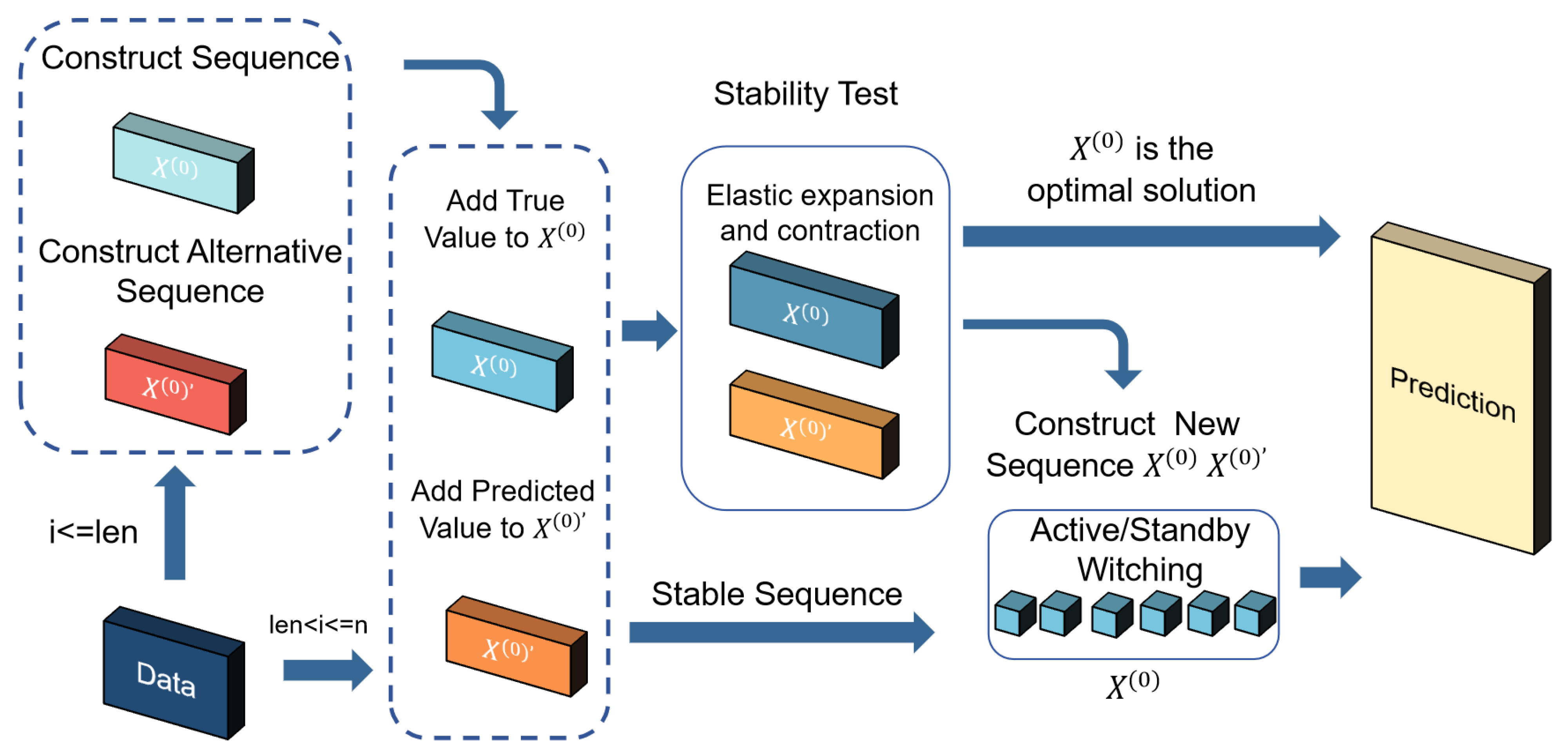
3.2. The Elastic Optimal Adaptive GM(1,1) Model

The elastic optimal adaptive GM(1,1) model (EOAGM) enhances the prediction accuracy of gray systems through parameter optimization methods. As illustrated in Figure 1, the EOAGM model is structured into three main steps:
  • Sequences construction: This step involves generating two types of sequences, the original sequence and the candidate sequence, to ensure robust prediction capability.
  • Stationarity detection: The EOAGM model improves on the AGM by using the ADF test to evaluate the stability of sequences. Stationarity ensures the model’s parameters accurately represent the system’s behavior, leading to better prediction accuracy.
  • Optimal sequence selection: This step identifies the sequence that provides the best prediction accuracy by evaluating the performance of both original and candidate sequences.

3.2.1. Sequences Construction

The process of sequence construction involves generating the original sequence and the candidate sequence, each designed to optimize prediction performance. The variable l e n (length) is initialized to represent the number of elements in the sequence. The steps of sequence construction include the following:
  • Defining sequence length: The optimal length l e n is set for both the original and candidate sequences.
  • Data insertion: When the sequence length is not more than l e n , new data points are directly added to both sequences. When the sequence length exceeds l e n , the observed value is appended to the original sequence, while the predicted value is added to the candidate sequence.
  • Maintaining sequence length: To keep the sequence length fixed, the oldest value is discarded from both sequences.
  • Temporary storage of discarded values: Discarded values are stored temporarily, allowing the model to revert to previous states during the stationarity detection phase if instability is detected. This structured approach ensures the sequences are robust, adaptable, and ready for subsequent stationarity detection and optimization steps.

3.2.2. Stationarity Detection

In the AGM, the length of the data sequence used to calculate the model parameters α and μ is fixed. However, even with operations that involve discarding outdated data and incorporating new data, the sequence stability may still degrade, leading to poor model performance and inaccurate predictions. To address this limitation, we introduce the ADF test method to assess the stability of the sequence within the model.
The ADF test is a statistical method used to determine whether a time series has a unit root, which indicates non-stationarity.
The procedure for calculating ADF statistics to test for the presence of unit roots is shown in Equation (7).
Y t = c + β t + α Y t 1 + ϕ Δ Y t 1 + e t , t = 0 , 1 , 2 , , n .
In the traditional DF test, the value of the time series at time t is denoted as Y t , the first-order difference of the series at time t 1 is denoted as Δ Y t 1 , and the difference term is e t . In traditional DF detection, an enhancement is made, transforming it as shown in Equation (8).
ϕ Δ Y t 1 = ϕ 1 Δ Y t 1 + ϕ 2 Δ Y t 2 + + ϕ p 1 Δ Y t ( p 1 ) ) , t = 0 , 1 , 2 , , n .
When conducting an ADF test, we typically pay attention to the test statistic ( T v a l u e ), the probability of the sequence being non-stationary ( P v a l u e ), and the critical values ( C v a l u e ) associated with the confidence interval [51].
The ADF test indicates whether the sequence has a unit root. A T v a l u e smaller than the C v a l u e implies stationarity. P v a l u e measures the probability of the sequence being non-stationary, with a P v a l u e < 0.05 indicating stationarity. The ADF test results provide C v a l u e s at different confidence levels (e.g., 1%, 5%, and 10%), which are used to compare with the T v a l u e . In the ADF test, the critical values of the confidence interval help us determine whether the time series is stationary, rather than directly providing a confidence interval for a parameter.
Modern statistical software packages, including including R (4.3.0+), Python (3.7), employ automated algorithms to select optimal lag orders for Dickey–Fuller tests based on predefined distribution criteria. In econometric analysis, the lag order specification in the augmented Dickey–Fuller (ADF) test is pivotal to ensure the validity of stationarity conclusions. For this study, the lag order was algorithmically determined via the Akaike information criterion (AIC) using Python’s statsmodels library, which generated the C v a l u e s and P v a l u e . The AIC optimizes model parsimony by penalizing over-parameterization, thereby mitigating risks of underfitting (insufficient lags) and overfitting (redundant lags). Furthermore, the AIC’s systematic optimization ensures that the selected lags adequately account for serial correlation in the residuals, which is critical for valid inference.
Using the ADF test, we assess whether adaptive adjustments to the sequence maintain its stability. Based on the test results, decisions can be made to modify the sequence length if necessary. If the adjusted sequence fails to achieve stationarity, the original sequence length is preserved.
The elastic adjustment process, as outlined in Algorithm 1, incorporates several parameters: c f , representing the confidence level (e.g., 1%, 5%, or and 10%, corresponding to 99%, 95%, and 90% probabilities of stationarity, respectively); d f  [52], indicating the differencing order, which can be first-order or second-order differencing for non-stationary time series data [53]. The ADF test method is applied to the sequence, yielding a result array containing T v a l u e , C v a l u e and P v a l u e , which collectively determine stationarity. To evaluate this, the stationarity method examines the array: if P v a l u e < 0.05 and T v a l u e < C v a l u e , the sequence is deemed stationary; otherwise, it is considered non-stationary. For non-stationary sequences, adjustments involve creating two new sequences (one by adding a data point to the beginning of the original sequence and the other by removing the oldest data point) and applying the ADF test to both. The sequence with the smaller P v a l u e is selected for further evaluation using the stationarity method. If the sequence achieves stationarity, it is used for subsequent modeling; otherwise, the original sequence is retained. This iterative approach ensures the balance and robustness of the sequence for accurate forecasting. In the revised methodology, it is adjusted up to two times during a single prediction cycle, and the window length is reset to its original baseline before initiating the next detection cycle.
Algorithm 1: Elastic adjustment process.
Electronics 14 02071 i001

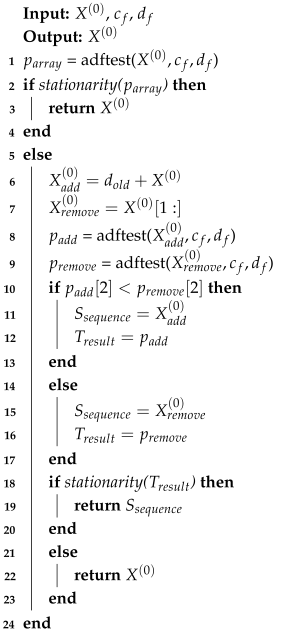
3.2.3. Optimal Sequence Selection

Stationarity detection adjusts the sequence length by adding or removing data from the sequence’s head to achieve a stable state. However, the sequence accepts all newly added values, including outliers or values with significant fluctuations, which would reduce the accuracy of the forecast result. Therefore, we employ the optimal sequence selection method to enhance prediction accuracy. The optimal sequence selection method is described in Algorithm 2. In Algorithm 2, we add a candidate series. Let the original series be a time series X k = i ( 0 ) with i observations. At the moment i + 1 , we obtain X ( 0 ) ( i + 1 ) , which is added to the original series and discard the oldest data to obtain a new series X k = i + 1 ( 0 ) , which serves as a prediction sequence, which is consistent with the AGM. In addition, we add the candidate series X k = i + 1 ( 0 ) = { X ( 0 ) ( 2 ) , , X ( 0 ) ( n ) , y p } .
At the moment i + 2 , we compare the true values with the predicted values of the two series, select a series with a small relative error, and then add new data, discard the old data, and generate a new candidate series right on top of the selection sequence.
The most useful thing about the candidate series is that the better data among the predicted data and the real data are selected for prediction, which leads to better prediction results.
Algorithm 2: Optimal sequence selection.
Electronics 14 02071 i002

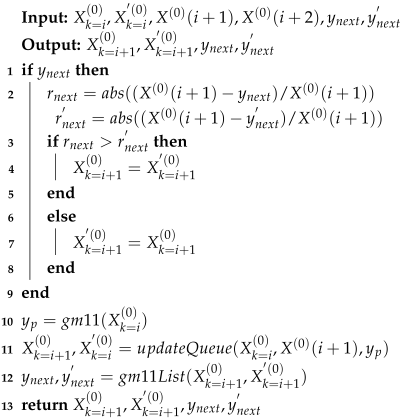
4. Experimental Results and Discussion

In this study, we first present the datasets, baseline methods, and evaluation metrics. Subsequently, we compare the prediction accuracy across different baseline approaches. Next, we conduct a sensitivity analysis to assess model robustness. Finally, we perform an ablation experiment to evaluate the contribution of key components.
Datasets: To validate the superiority of our algorithm, we conducted experiments on three distinct datasets: (1) China’s annual GDP data from 2008 to 2023, (2) district heating data from Jinan City, China, and (3) the annual cargo and mail throughput data of Jinan Yaoqiang Airport.
For the GDP dataset, obtained from the National Bureau of Statistics of China (https://data.stats.gov.cn (accessed on 22 May 2024)), we utilized observations from the years 2008–2014 as the training set to predict subsequent values for 2015–2021. For the heating dataset, we selected daily measurements from six residential buildings between 1–13 January. The model was trained on data from 1–7 January and tested on its ability to forecast heating demand for 8–13 January. The raw district heating data are presented in Table 1. Column 1 represents observation dates, and columns 2–7 represent daily thermal energy consumption (kWh) for buildings 11–16. For the cargo and mail throughput data of Jinan Yaoqiang Airport (JYA-CMTD), obtained from the website (https://www.huaon.com/channel/industrydata/1060968.html (accessed on 5 January 2025)), we utilized observations from 2011–2016 as the training set to predict subsequent years’ values for 2017–2021.
To promote transparency and reproducibility in scientific research, the original datasets and supplementary materials associated with this article were deposited in a public repository. The resources are freely accessible via Gitee and the link is https://gitee.com/sduliteng/gm.git (accessed on 10 May 2025).
Baseline Method: In addition to the traditional GM(1,1) (TGM), this study comprehensively evaluates five advanced gray models and one non-gray model proposed in recent studies.
  • Cumulative GM(1,1) Model (CGM) [54]: The CGM recalculates α and μ iteratively by incorporating new data. While this method improves adaptability by considering growing datasets, the increasing sequence length may introduce noise and irrelevant information, reducing prediction precision over time.
  • Adaptive GM(1,1) Model (AGM) [22]: The AGM dynamically adjusts the data sequence by discarding older data and incorporating new observations. This approach enhances forecasting accuracy for dynamic systems by reflecting real-time changes. However, removing older data may destabilize predictions, and incorporating new data (including anomalies) may reduce prediction reliability.
  • Simultaneous Gray Model (SimGM) [42]: This model can improve the algorithm for calculating α and μ [55]. Traditional GM(1,1) employs ordinary least squares (OLS) to estimate α and μ . However, since real-world systems are governed by interconnected and evolving factors, a single differential equation may inadequately capture these relationships. To address this limitation, the SimGM has been proposed, which significantly improves prediction accuracy compared to conventional single-equation models.
  • Nonlinear Gray Model (NonlGM) [56]: The NonlGM proposes an enhanced GM(1,N) model incorporating nonlinear optimization techniques to improve forecasting accuracy and robustness. The background value in the TGM(1,1) model is defined as Z ( 1 ) ( K ) = 0.5 X ( 1 ) ( K ) + 0.5 X ( 1 ) ( K 1 ) , k = 2 , , n . In the process of background value optimization, the fixed weight coefficient (0.5) can be optimized. In the NonlGM, Z ( 1 ) ( K ) = a X ( 1 ) ( K ) + ( 1 a ) X ( 1 ) ( K 1 ) , where a is optimized.
  • Improved Gray Model (ImGM) [37]: This model is an improved optimized background value determination method for the GM(1,1) model. In this method, background value optimization can also be achieved through the exponential background value and dynamic adaptive background value using data characteristics methods.
  • Lagged [57]: This model employs a non-gray modeling approach for data forecasting, specifically utilizing a quantile regression framework with lagged and asymmetric effects.
Evaluation Metrics: In the experiment, relative error and mean error are used as test indicators. The formula for calculating relative error is as follows:
w k = X ^ ( 0 ) ( k ) X ( 0 ) ( k ) X ( 0 ) ( k ) ,
where X ^ ( 0 ) ( k ) is the predicted value of the k-th data point, and X ( 0 ) ( k ) is the true value of the k-th data point. Assuming n is the number of predicted values, then the average error of the prediction is as follows:
w a v g = n k = 1 w k n .
Common Parameter Settings: In the experiments, the baseline models incorporate several shared parameters to ensure consistency and comparability. For the GM(1,1) model, the initialization parameters are uniformly set as gm11.alpha = 0.5, gm11.convolution = True, and gm11.stride = 1 across all datasets. These configurations aim to balance model flexibility and computational efficiency. For the ADF algorithm, parameters regression = “c” (constant term included) and autolag = “AIC” (automatic lag selection via the Akaike information criterion) are adopted universally to standardize stationarity testing and enhance robustness in time series analysis.
Dataset-Specific Configurations: The sequence length in GM(1,1) is optimized based on empirical results: a length of seven minimizes prediction errors for forecasting China’s GDP and Jinan’s thermal energy consumption, while six is optimal for the annual cargo and mail throughput data of Jinan Yaoqiang Airport. In the ADF algorithm, differencing strategies vary: thermal energy and cargo throughput data use first-order differencing, whereas GDP data employs first-order differencing for sequences shorter than six and second-order differencing for longer sequences to address non-stationarity. Elastic scaling ranges also differ: thermal energy and cargo throughput are assigned a range of 1, while GDP uses 2 to accommodate its higher volatility.
Rationale for Optimality: Parameter selections are empirically validated. For GM(1,1), a sequence length of seven optimally captures temporal patterns in GDP and thermal energy data, balancing underfitting and overfitting risks. A shorter length of six for cargo throughput aligns with its lower seasonal complexity. In ADF, differencing orders are tailored to data characteristics: higher-order differencing for longer GDP sequences mitigates trend persistence, while first-order suffices for other datasets. Elastic ranges reflect inherent volatility, i.e., GDP’s broader range of 2 accommodates macroeconomic fluctuations, whereas thermal and cargo data’s narrower range of 1 suits their smoother trends. These settings collectively ensure model generalizability and precision across diverse datasets.

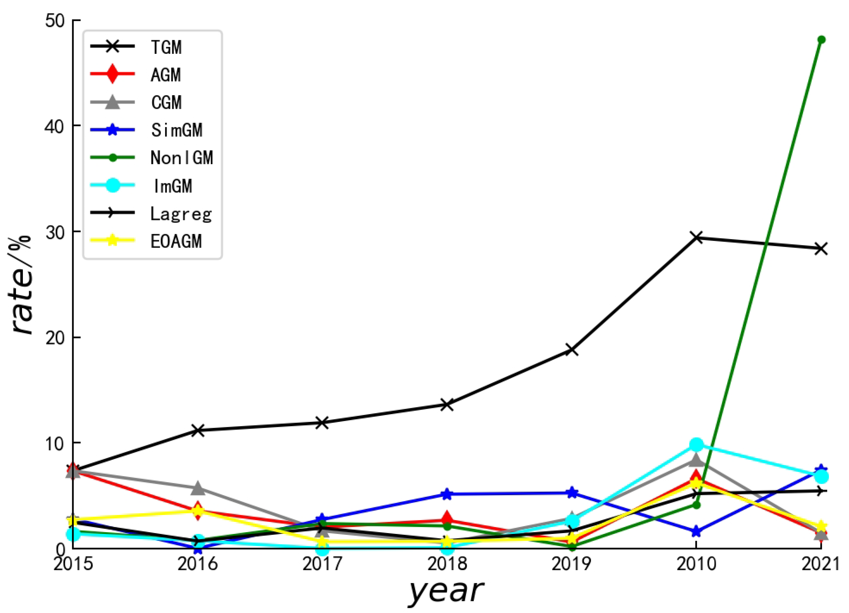
4.1. Performance Comparison with Base Lines

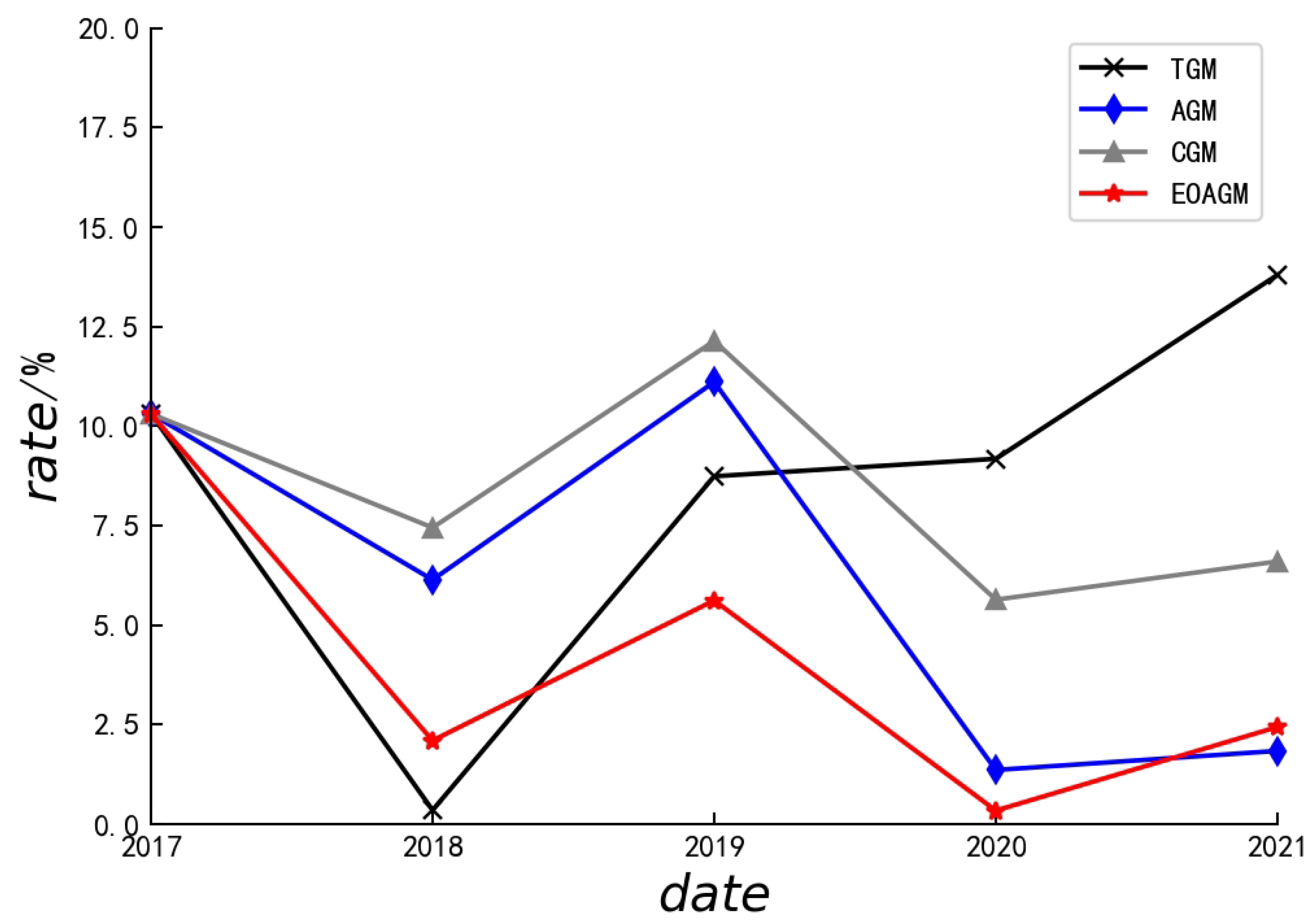
4.1.1. National GDP Prediction

To demonstrate the general applicability of our proposed model, we performed a comprehensive forecasting of China’s GDP from 2015 to 2021 using eight gray models: TGM/CGM/AGM/SimGM/NonlGM/ImGM/Lagreg and EOAGM.
The errors (%) of each model for different years, as well as the mean errors, are presented in Table 2. As can be observed from Table 2, our algorithm achieves the smallest values in both mean error and maximum error.
As Table 2 shows, error differences of <1 % can be seen between EOAGM and AGM for four of the GDP years. We provide a paired Wilcoxon signed-rank test over all forecasting horizons to show significance. The test was performed on the paired error data (before = AGM errors and after = EOAGM errors) from 2015 to 2024, yielding a p-value of 0.0499. Since this value is below the significance threshold of 0.05, we reject the null hypothesis and conclude that the improvement in EOAGM over AGM is statistically significant.
Furthermore, a line chart (Figure 2) was employed to illustrate the stability of the algorithms. The yellow line represents the error trend of our proposed algorithm, demonstrating its exceptional stability.

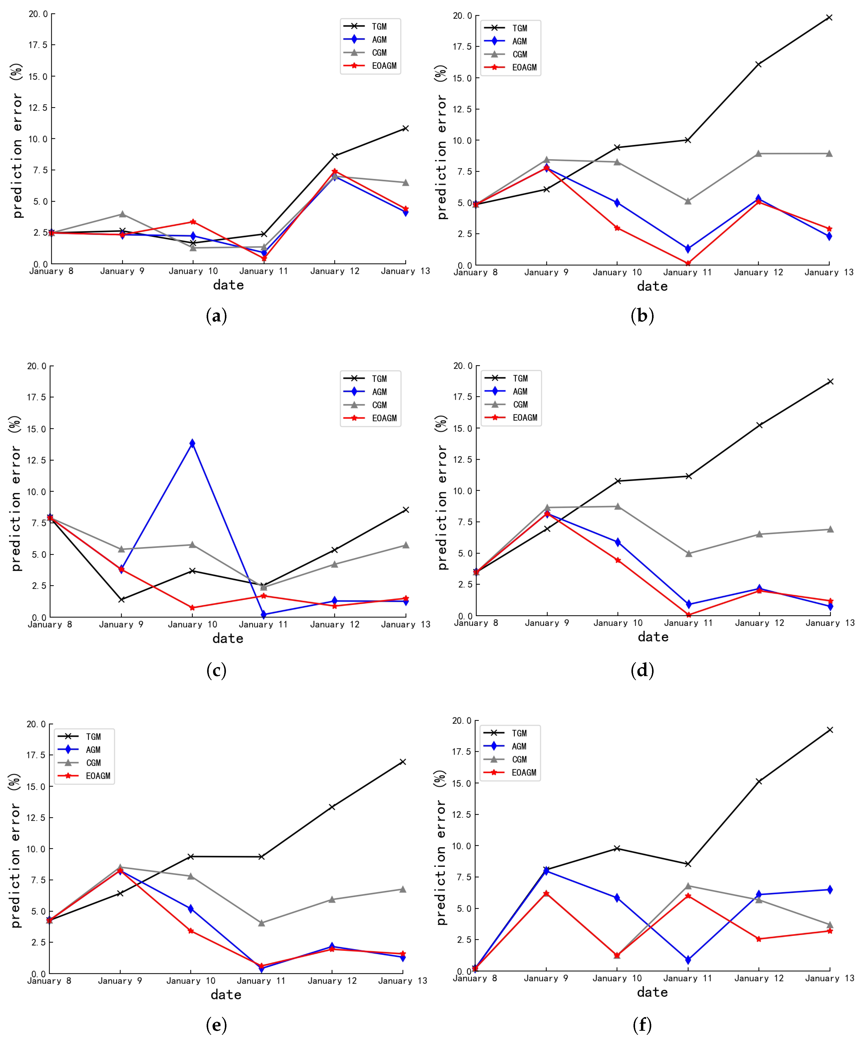
4.1.2. Indigenous Thermal Energy Prediction

TGM/CGM/AGM and EOAGM were applied to forecast indigenous thermal energy prediction for six buildings over the period from 8 to 13 January. The raw data presented in Table 1 were processed using Equation (9) to calculate daily prediction errors. For example, for the 8 January prediction error, the thermal load data on that date was predicted using either the preceding 6-day or 7-day sequences (with sequence length adjusted based on balance test results), yielding the predicted value X ^ ( 0 ) ( k ) . The observed value X ( 0 ) ( k ) , corresponding to 8 January, was directly extracted from the 8 January entry in Table 1. Figure 3 explicitly visualizes these errors from 8 to 13 January through line charts, enabling quantitative comparison of algorithmic accuracy (mean absolute error) and stability (temporal error variance).
As shown in Figure 3, both AGM and EOAGM outperform TGM and CGM. Furthermore, EOAGM consistently surpasses the adaptive model in prediction accuracy.
Using the mean error as a test indicator for the four algorithms, as shown in Table 3, except for building 11, the average error of the EOAGM is the smallest in the other five buildings. Moreover, if the data fluctuate or there are anomalous data, the prediction accuracy of the EOAGM will be significantly improved.

4.1.3. JYA-CMTD Prediction

To validate the universal applicability of our proposed model, we conducted comprehensive predictions of JYA-CMTD from 2017 to 2021 using TGM/CGM/AGM and EOAGM.
The errors (%) of each model for different years, as well as the mean errors, are presented in Table 4. As can be observed from Table 4, our algorithm achieves the smallest values in both mean error and maximum error, improving precision by at least 2.6% compared to baseline methods.
Furthermore, a line chart (Figure 4) was employed to illustrate the stability of the algorithms. The red line represents the error trend of our proposed algorithm, demonstrating its exceptional stability.

4.1.4. On Model Comparison

As demonstrated in Table 2, Table 3 and Table 4, the proposed EOAGM model exhibits superior performance compared to the seven baseline methods. This enhanced performance can be attributed to the following key innovations:
Stability-Aware Adaptive Forecasting: The model incorporates stationarity testing and dynamic sequence length adjustment, effectively mitigating prediction errors caused by temporal fluctuations. This ensures robust performance under non-stationary conditions.
Predictive Parameter Optimization: A novel parameter optimization strategy is implemented by embedding predicted values into candidate sequences. This approach allows for the direct evaluation of their predictive efficacy in subsequent forecasting steps, thereby enhancing both adaptability and precision in dynamic system modeling.

4.2. Ablation Experiment

In this section, we perform necessary ablation studies by removing specific components to generate three ablation models.
  • EOAGM-A: We replace the dynamic adaptive adjustment of sequences with a cumulative aggregation mode for data prediction.
  • EOAGM-O: We remove optimal sequence selection for data prediction.
  • EOAGM-E: We omit stationarity detection for data prediction.
As can be seen from Table 5, removing one of the three components affects the accuracy of the algorithm’s prediction.

5. Conclusions

To overcome challenges related to prediction instability and noise sensitivity in the TGM, this study proposes the EOAGM, an enhanced version of the AGM. Firstly, we replace the traditional cumulative generation sequence with an adaptive sequence generation method, which enhances the model’s ability to manage dynamic time series. Secondly, a stationarity detection method is introduced to adjust the sequence length dynamically, shifting from fixed-length to elastic sequences to reduce the impact of data fluctuations. Finally, the parameter optimization process is improved by incorporating predicted values into the candidate sequence. This allows for evaluating whether the inclusion of predicted values in subsequent forecasts improves performance, particularly in the presence of data volatility or anomalies. By selecting the optimal sequence, the proposed model significantly improves both simulation accuracy and predictive precision. The EOAGM was empirically validated in the Jinan Municipal Thermal Energy System, demonstrating robust performance in addressing nonlinear dynamics and operational uncertainties. Furthermore, the model exhibits inherent versatility for domains requiring high-fidelity time series analysis. For instance, in airline operations, the EOAGM enables accurate forecasting of monthly passenger volumes, which is critical for optimizing fleet scheduling, crew allocation, and revenue management under seasonal variations or exogenous disturbances. Similarly, as for power grid systems, high-frequency financial trading, and pattern prediction systems [58,59,60], it can predict monthly electricity generation patterns to mitigate supply–demand imbalances, enhance grid resilience, and facilitate renewable energy integration. These applications leverage the model’s capacity to disentangle complex temporal dependencies while adaptively incorporating external covariates.

Author Contributions

Conceptualization, T.L. and Z.L.; methodology, T.L. and Z.L.; software, T.L. and J.N.; validation, G.Q., T.L., and C.J.; formal analysis, X.L. and Z.L.; investigation, X.L. and Z.L.; resources, X.L. and Z.L.; data curation, T.L.; writing—original draft, C.J.; writing—review and editing, G.Q.; visualization, T.L.; supervision, J.N. and Z.L.; project administration, T.L. All authors have read and agreed to the published version of the manuscript.

Funding

This research was funded by the National Natural Science Foundation of China grant numbers 62276155 and 62206157.

Data Availability Statement

The data presented in this study are available on request from the corresponding author.

Acknowledgments

The authors are grateful to the editors and reviewers for their constructive comments, which have significantly improved this work.

Conflicts of Interest

The authors declare no conflicts of interest.

References

  1. Alqahtani, A.; Ali, M.; Xie, X.; Jones, M.W. Deep time-series clustering: A review. Electronics 2021, 10, 3001. [Google Scholar] [CrossRef]
  2. Hu, Y.; Zhan, P.; Xu, Y.; Zhao, J.; Li, Y.; Li, X. Temporal representation learning for time series classification. Neural Comput. Appl. 2021, 33, 3169–3182. [Google Scholar] [CrossRef]
  3. Liu, F.; Chen, L.; Zheng, Y.; Feng, Y. A prediction method with data leakage suppression for time series. Electronics 2022, 11, 3701. [Google Scholar] [CrossRef]
  4. Wei, Y.; Wang, Y.; Du, M.; Hu, Y.; Ji, C. Adaptive shapelet selection for time series classification. In Proceedings of the International Conference on Computer Supported Cooperative Work in Design, Rio de Janeiro, Brazil, 24–26 May 2023; pp. 1607–1612. [Google Scholar]
  5. Hu, Y.; Ji, C.; Jing, M.; Ding, Y.; Kuai, S.; Li, X. A continuous segmentation algorithm for streaming time series. In Proceedings of the Collaborate Computing: Networking, Applications and Worksharing: 12th International Conference, CollaborateCom 2016, Beijing, China, 10–11 November 2016; Proceedings 12. Springer: Berlin/Heidelberg, Germany, 2017; pp. 140–151. [Google Scholar]
  6. Ji, C.; Hu, Y.; Liu, S.; Pan, L.; Li, B.; Zheng, X. Fully convolutional networks with shapelet features for time series classification. Inf. Sci. 2022, 612, 835–847. [Google Scholar] [CrossRef]
  7. Hu, Y.; Ren, P.; Luo, W.; Zhan, P.; Li, X. Multi-resolution representation with recurrent neural networks application for streaming time series in IoT. Comput. Netw. 2019, 152, 114–132. [Google Scholar] [CrossRef]
  8. Hu, Y.; Jiang, Z.; Zhan, P.; Zhang, Q.; Ding, Y.; Li, X. A novel multi-resolution representation for streaming time series. Procedia Comput. Sci. 2018, 129, 178–184. [Google Scholar] [CrossRef]
  9. Liu, F.; Yin, B.; Cheng, M.; Feng, Y. n-Dimensional chaotic time series prediction method. Electronics 2022, 12, 160. [Google Scholar] [CrossRef]
  10. Wan, R.; Tian, C.; Zhang, W.; Deng, W.; Yang, F. A multivariate temporal convolutional attention network for time-series forecasting. Electronics 2022, 11, 1516. [Google Scholar] [CrossRef]
  11. Kim, M.; Lee, S.; Jeong, T. Time series prediction methodology and ensemble model using real-world data. Electronics 2023, 12, 2811. [Google Scholar] [CrossRef]
  12. Yuan, H.; Liao, S. A time series-based approach to elastic kubernetes scaling. Electronics 2024, 13, 285. [Google Scholar] [CrossRef]
  13. Li, G.; Yang, Z.; Wan, H.; Li, M. Anomaly-PTG: A time series data-anomaly-detection transformer framework in multiple scenarios. Electronics 2022, 11, 3955. [Google Scholar] [CrossRef]
  14. Zhong, Y.; He, T.; Mao, Z. Enhanced Solar Power Prediction Using Attention-Based DiPLS-BiLSTM Model. Electronics 2024, 13, 4815. [Google Scholar] [CrossRef]
  15. Ma, X.; Chang, S.; Zhan, J.; Zhang, L. Advanced Predictive Modeling of Tight Gas Production Leveraging Transfer Learning Techniques. Electronics 2024, 13, 4750. [Google Scholar] [CrossRef]
  16. Dai, L.; Liu, J.; Ju, Z. Attention Mechanism and Bidirectional Long Short-Term Memory-Based Real-Time Gaze Tracking. Electronics 2024, 13, 4599. [Google Scholar] [CrossRef]
  17. Hu, Y.; Liu, M.; Su, X.; Gao, Z.; Nie, L. Video moment localization via deep cross-modal hashing. IEEE Trans. Image Process. 2021, 30, 4667–4677. [Google Scholar] [CrossRef]
  18. Zeng, B.; Luo, C.; Liu, S.; Bai, Y.; Li, C. Development of an optimization method for the GM(1,N) model. Eng. Appl. Artif. Intell. 2016, 55, 353–362. [Google Scholar] [CrossRef]
  19. Masini, R.P.; Medeiros, M.C.; Mendes, E.F. Machine learning advances for time series forecasting. J. Econ. Surv. 2023, 37, 76–111. [Google Scholar] [CrossRef]
  20. Molnár, A.; Csiszárik-Kocsir, Á. Forecasting economic growth with v4 countries’ composite stock market indexes—A granger causality test. Acta Polytech. Hung. 2023, 20, 135–154. [Google Scholar] [CrossRef]
  21. Wang, Z.X.; Li, Q.; Pei, L.L. A seasonal GM(1,1) model for forecasting the electricity consumption of the primary economic sectors. Energy 2018, 154, 522–534. [Google Scholar] [CrossRef]
  22. Fan, G.; Li, B.; Mu, W.; Ji, C. The Application of the Optimal GM(1,1) Model for Heating Load Forecasting. In Proceedings of the 2015 4th International Conference on Mechatronics, Materials, Chemistry and Computer Engineering, Xi’an, China, 12–13 December 2015; Atlantis Press: Paris, France, 2015. [Google Scholar]
  23. Ren, Y.; Xia, L.; Wang, Y. An improved GM(1,1) forecasting model based on Aquila Optimizer for wind power generation in Sichuan Province. Soft Comput. 2024, 28, 8785–8805. [Google Scholar] [CrossRef]
  24. Prakash, S.; Agrawal, A.; Singh, R.; Singh, R.K.; Zindani, D. A decade of grey systems: Theory and application–bibliometric overview and future research directions. Grey Syst. Theory Appl. 2023, 13, 14–33. [Google Scholar] [CrossRef]
  25. Cai, L.; Wu, F.; Lei, D. Pavement condition index prediction using fractional order GM(1,1) model. IEEE Trans. Electr. Electron. Eng. 2021, 16, 1099–1103. [Google Scholar] [CrossRef]
  26. Ding, S. A novel self-adapting intelligent grey model for forecasting China’s natural-gas demand. Energy 2018, 162, 393–407. [Google Scholar] [CrossRef]
  27. Han, H.; Jing, Z. Anomaly Detection in Wireless Sensor Networks Based on Improved GM Model. Teh. Vjesn. 2023, 30, 1265–1273. [Google Scholar]
  28. Javanmardi, E.; Liu, S.; Xie, N. Exploring the challenges to sustainable development from the perspective of grey systems theory. Systems 2023, 11, 70. [Google Scholar] [CrossRef]
  29. Zhang, K.; Yuan, B. Dynamic change analysis and forecast of forestry-based industrial structure in China based on grey systems theory. J. Sustain. For. 2020, 39, 309–330. [Google Scholar] [CrossRef]
  30. Cheng, M.; Liu, B. Application of a novel grey model GM (1,1, exp× sin, exp× cos) in China’s GDP per capita prediction. Soft Comput. 2024, 28, 2309–2323. [Google Scholar] [CrossRef]
  31. Wang, Z.X.; Wang, Z.W.; Li, Q. Forecasting the industrial solar energy consumption using a novel seasonal GM(1,1) model with dynamic seasonal adjustment factors. Energy 2020, 200, 117460. [Google Scholar] [CrossRef]
  32. Julong, D. Introduction to grey system theory. J. Grey Syst. 1989, 1, 1–24. [Google Scholar]
  33. Li, J.; Feng, S.; Zhang, T.; Ma, L.; Shi, X.; Zhou, X. Study of Long-Term Energy Storage System Capacity Configuration Based on Improved Grey Forecasting Model. IEEE Access 2023, 11, 34977–34989. [Google Scholar] [CrossRef]
  34. Delcea, C.; Javed, S.A.; Florescu, M.S.; Ioanas, C.; Cotfas, L.A. 35 years of grey system theory in economics and education. Kybernetes 2025, 54, 649–683. [Google Scholar] [CrossRef]
  35. Chia-Nan, W.; Nhu-Ty, N.; Thanh-Tuyen, T. Integrated DEA Models and Grey System Theory to Evaluate Past-to-Future Performance: A Case of Indian Electricity Industry. Sci. World J. 2015, 2015, 638710. [Google Scholar]
  36. Zhan, T.; Xu, H. Nonlinear optimization of GM(1,1) model based on multi-parameter background value. In Proceedings of the International Conference on Computer and Computing Technologies in Agriculture, Beijing, China, 29–31 October 2011; Springer: Berlin/Heidelberg, Germany, 2011; pp. 15–19. [Google Scholar]
  37. Ma, Y.; Wang, S. Construction and application of improved GM(1,1) power model. J. Quant. Econ. 2019, 36, 84–88. [Google Scholar]
  38. Chen, F.; Zhu, Y. A New GM(1,1) Based on Piecewise Rational Linear/linear Monotonicity-preserving Interpolation Spline. Eng. Lett. 2021, 29, 3. [Google Scholar]
  39. Wang, X.; Qi, L.; Chen, C.; Tang, J.; Jiang, M. Grey System Theory based prediction for topic trend on Internet. Eng. Appl. Artif. Intell. 2014, 29, 191–200. [Google Scholar] [CrossRef]
  40. Liu, S.; Tao, L.; Xie, N.; Yang, Y. On the new model system and framework of grey system theory. In Proceedings of the 2015 IEEE International Conference on Grey Systems and Intelligent Services (GSIS), Leicester, UK, 18–20 August 2015; pp. 1–11. [Google Scholar]
  41. Tang, L.; Lu, Y. An Improved Non-equal Interval GM(1,1) Model Based on Grey Derivative and Accumulation. J. Grey Syst. 2020, 32, 77. [Google Scholar]
  42. Cheng, M.; Cheng, Z. A novel simultaneous grey model parameter optimization method and its application to predicting private car ownership and transportation economy. J. Ind. Manag. Optim. 2023, 19, 3160–3171. [Google Scholar] [CrossRef]
  43. Zeng, X.; Xu, M.; Hu, Y.; Tang, H.; Hu, Y.; Nie, L. Adaptive edge-aware semantic interaction network for salient object detection in optical remote sensing images. IEEE Trans. Geosci. Remote Sens. 2023, 61, 1–16. [Google Scholar] [CrossRef]
  44. Yuhong, W.; Jie, L. Improvement and application of GM(1,1) model based on multivariable dynamic optimization. J. Syst. Eng. Electron. 2020, 31, 593–601. [Google Scholar] [CrossRef]
  45. Gianfreda, A.; Maranzano, P.; Parisio, L.; Pelagatti, M. Testing for integration and cointegration when time series are observed with noise. Econ. Model. 2023, 125, 106352. [Google Scholar] [CrossRef]
  46. Chang, Y.; Park, J.Y. On the asymptotics of ADF tests for unit roots. Econom. Rev. 2002, 21, 431–447. [Google Scholar] [CrossRef]
  47. Alam, M.B.; Hossain, M.S. Investigating the connections between China’s economic growth, use of renewable energy, and research and development concerning CO2 emissions: An ARDL Bound Test Approach. Technol. Forecast. Soc. Change 2024, 201, 123220. [Google Scholar] [CrossRef]
  48. Hassan, M.K.; Kazak, H.; Adıgüzel, U.; Gunduz, M.A.; Akcan, A.T. Convergence in Islamic financial development: Evidence from Islamic countries using the Fourier panel KPSS stationarity test. Borsa Istanb. Rev. 2023, 23, 1289–1302. [Google Scholar] [CrossRef]
  49. Lin, J.X.; Chen, G.; Pan, H.S.; Wang, Y.C.; Guo, Y.C.; Jiang, Z.X. Analysis of stress-strain behavior in engineered geopolymer composites reinforced with hybrid PE-PP fibers: A focus on cracking characteristics. Compos. Struct. 2023, 323, 117437. [Google Scholar] [CrossRef]
  50. Asgari, H.; Moridian, A.; Havasbeigi, F. The Impact of Economic Complexity on Income Inequality with Emphasis on the Role of Human Development Index in Iran’s Economy with ARDL Bootstrap Approach. J. Dev. Cap. 2024, 9, 35–56. [Google Scholar]
  51. Yung, Y.F.; Bentler, P.M. Bootstrap-corrected ADF test statistics in covariance structure analysis. Br. J. Math. Stat. Psychol. 1994, 47, 63–84. [Google Scholar] [CrossRef]
  52. Tian, W.; Zhou, H.; Deng, W. A class of second order difference approximations for solving space fractional diffusion equations. Math. Comput. 2015, 84, 1703–1727. [Google Scholar] [CrossRef]
  53. Guo, Z.; Yu, J. The existence of periodic and subharmonic solutions of subquadratic second order difference equations. J. Lond. Math. Soc. 2003, 68, 419–430. [Google Scholar] [CrossRef]
  54. Liu, S.F.; Forrest, J. Advances in grey systems theory and its applications. In Proceedings of the 2007 IEEE International Conference on Grey Systems and Intelligent Services, Nanjing, China, 18–20 November 2007; pp. 1–6. [Google Scholar]
  55. Romano, J.L.; Kromrey, J.D.; Owens, C.M.; Scott, H.M. Confidence interval methods for coefficient alpha on the basis of discrete, ordinal response items: Which one, if any, is the best? J. Exp. Educ. 2011, 79, 382–403. [Google Scholar] [CrossRef]
  56. Fu, Z.; Yang, Y.; Wang, T. Prediction of urban water demand in Haiyan county based on improved nonlinear optimization GM (1, N) model. Water Resour. Power 2019, 37, 44–47. [Google Scholar]
  57. Dawar, I.; Dutta, A.; Bouri, E.; Saeed, T. Crude oil prices and clean energy stock indices: Lagged and asymmetric effects with quantile regression. Renew. Energy 2021, 163, 288–299. [Google Scholar] [CrossRef]
  58. Han, Y.; Hu, Y.; Song, X.; Tang, H.; Xu, M.; Nie, L. Exploiting the social-like prior in transformer for visual reasoning. In Proceedings of the AAAI Conference on Artificial Intelligence, Vancouver, BC, Canada, 20–27 February 2024; Volume 38, pp. 2058–2066. [Google Scholar]
  59. Tang, H.; Hu, Y.; Wang, Y.; Zhang, S.; Xu, M.; Zhu, J.; Zheng, Q. Listen as you wish: Fusion of audio and text for cross-modal event detection in smart cities. Inf. Fusion 2024, 110, 102460. [Google Scholar] [CrossRef]
  60. Hu, Y.; Wang, K.; Liu, M.; Tang, H.; Nie, L. Semantic collaborative learning for cross-modal moment localization. ACM Trans. Inf. Syst. 2023, 42, 1–26. [Google Scholar] [CrossRef]
Figure 1. General framework.
Electronics 14 02071 g001
Figure 2. Algorithmic errors in GDP.
Electronics 14 02071 g002
Figure 3. (a) represents the indigenous thermal energy prediction error for building No. 11 over the period from 8 to 13 January. (b) represents the indigenous thermal energy prediction error for building No. 12 over the period from 8 to 13 January. (c) represents the indigenous thermal energy prediction error for building No. 13 over the period from 8 to 13 January. (d) represents the indigenous thermal energy prediction error for building No. 14 over the period from 8 to 13 January. (e) represents the indigenous thermal energy prediction error for building No. 15 over the period from 8 to 13 January. (f) represents the indigenous thermal energy prediction error for building No. 16 over the period from 8 to 13 January.
Electronics 14 02071 g003
Figure 4. Algorithmic errors in JYA-CMTD.
Electronics 14 02071 g004
Table 1. Raw data of thermal energy consumption.
DateNo. 11No. 12No. 13No. 14No. 15No. 16
01-0113,900.293326.232536.822295.934926.7417,017.67
01-0213,556.133396.632530.542304.054882.5416,663.45
01-0313,209.103333.601914.242267.044844.1416,070.78
01-0412,385.613059.222964.362118.254544.0514,970.55
01-0512,313.993054.512338.642106.834535.8314,551.11
01-0613,223.573160.682366.732150.194633.1615,105.55
01-0713,267.333090.402349.922117.34585.9415,458.17
01-0812,532.192840.632218.291980.024277.2614,559.78
01-0913,145.063111.992423.012164.074703.2115,530.5
01-1012,972.853166.902475.542218.124793.1515,543.7
01-1113,024.713128.92441.322189.764729.3614,660.22
01-1213,868.683292.882509.362255.724882.8615,947.28
01-1314,165.043382.872591.212312.535029.0316,464.54
Table 2. Comparison of algorithmic errors in GDP analysis.
Errors (%)Algorithms
TGMAGMCGMSimGMNonlGMImGMLagregEOAGM
w 2015 7.367.367.362.81.631.402.482.72
w 2016 11.173.565.730.020.770.7490.7123.56
w 2017 11.912.031.682.752.373.27 × 10−51.950.65
w 2018 13.642.680.525.152.140.0780.7460.69
w 2019 18.80.622.865.260.202.601.680.98
w 2020 29.46.638.401.624.189.855.26.21
w 2021 28.41.491.487.4348.26.865.462.09
w a v g 17.2413.484.533.578.503.072.602.41
Table 3. Comparison of average error results.
AlgorithmsAverage Errors (%)
No. 11No. 12No. 13No. 14No. 15No. 16
TGM4.76 ± 3.9211.04 ± 5.824.902.8911.04 ± 5.499.95 ± 4.6110.16 ± 6.53
AGM3.17 ± 2.132.31 ± 3.924.71 ± 5.263.55 ± 2.93.60 ± 2.903.97 ± 3.22
CGM3.76 ± 2.517.42 ± 3.921.90 ± 1.846.54 ± 2.066.23 ± 1.834.58 ± 2.74
EOAGM3.39 ± 2.373.95 ± 2.573.06 ± 2.753.22 ± 2.883.34 ± 2.743.22 ± 2.45
Table 4. Comparison of algorithmic errors in JYA-CMTD analysis.
Errors (%)Algorithms
TGMAGMCGMEOAGM
w 2017 10.3110.3110.3110.31
w 2018 0.356.147.452.10
w 2019 8.7411.1112.145.62
w 2020 9.181.365.640.34
w 2021 13.801.846.602.44
w a v g 8.476.848.424.16
Table 5. Variants on benchmark datasets.
DatesetAverage Errors (%)
EOAGM-AEOAGM-OEOAGM-EEOAGM
w g d p 4.012.433.082.41
w a v g 11 3.483.173.393.39
w a v g 12 6.854.284.163.95
w a v g 13 4.874.533.213.06
w a v g 14 6.353.553.223.22
w a v g 15 5.913.603.343.34
w a v g 16 4.273.683.543.22
Disclaimer/Publisher’s Note: The statements, opinions and data contained in all publications are solely those of the individual author(s) and contributor(s) and not of MDPI and/or the editor(s). MDPI and/or the editor(s) disclaim responsibility for any injury to people or property resulting from any ideas, methods, instructions or products referred to in the content.

