
GPU-Optimized Implementation for Accelerating CSAR Imaging

Abstract
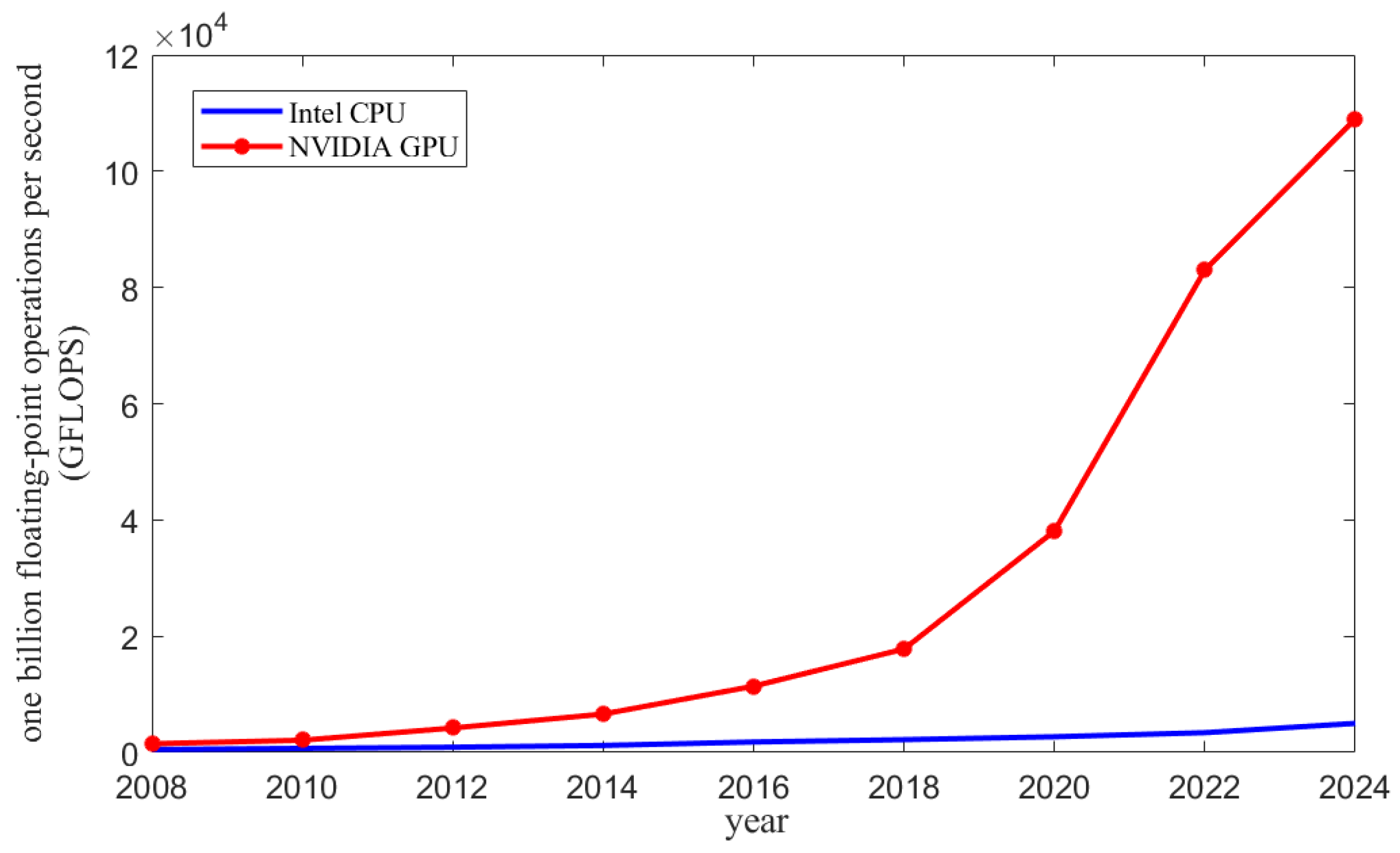
1. Introduction
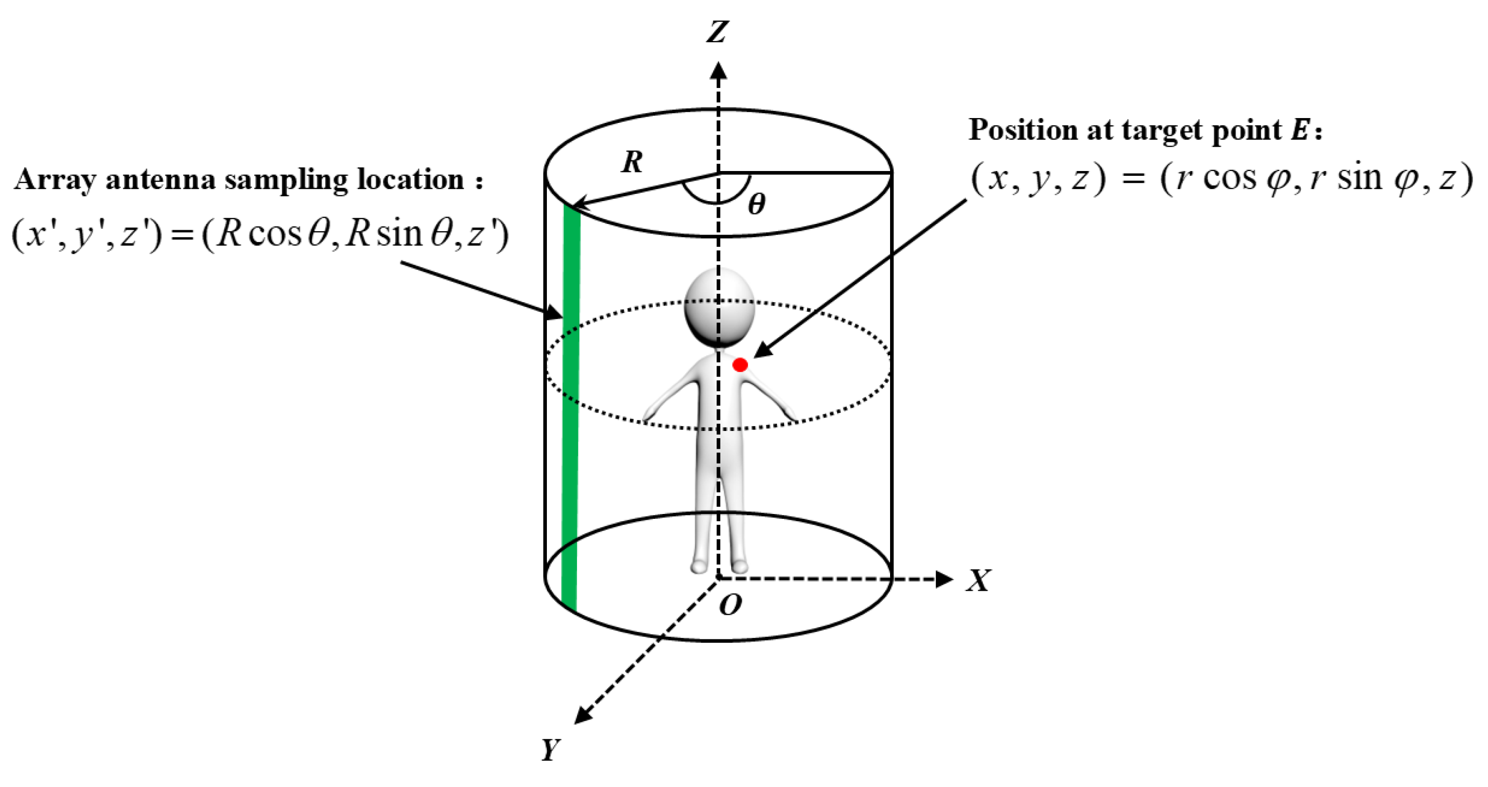
2. Three-Dimensional Cylindrical RMA
| Algorithm 1: Three-dimensional cylindrical RMA |
|
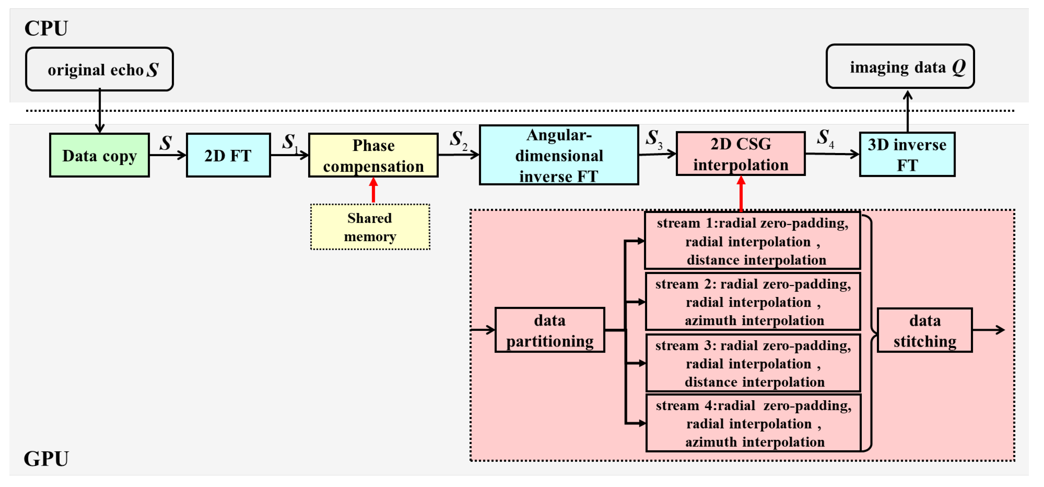
3. The Implementation on GPU
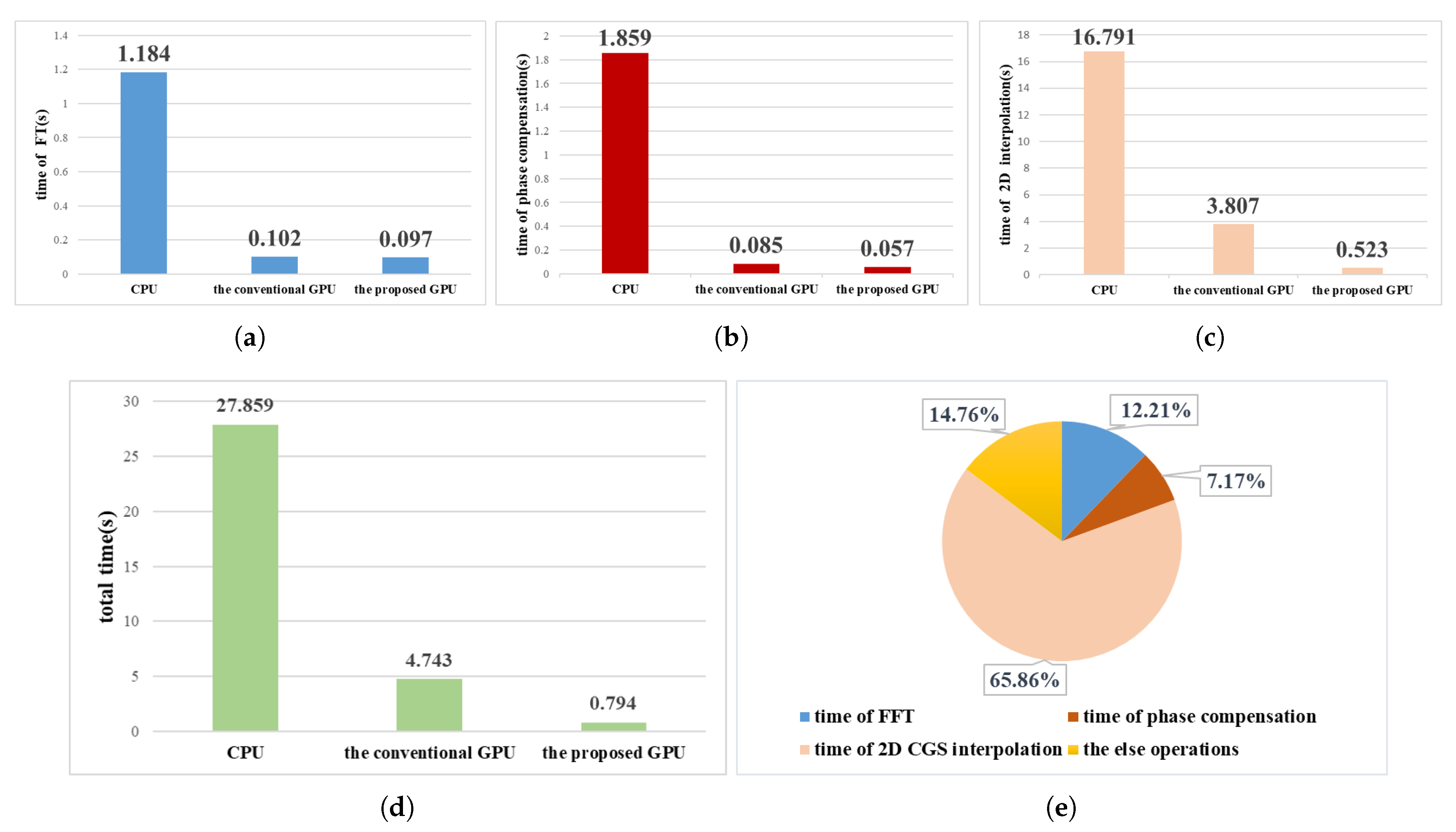
3.1. Fourier Transform
3.2. Phase Compensation
| Algorithm 2: Phase compensation |
|
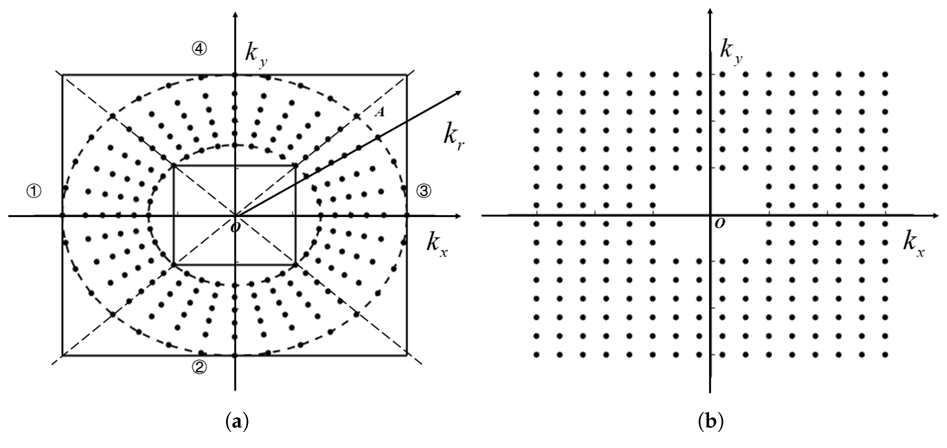
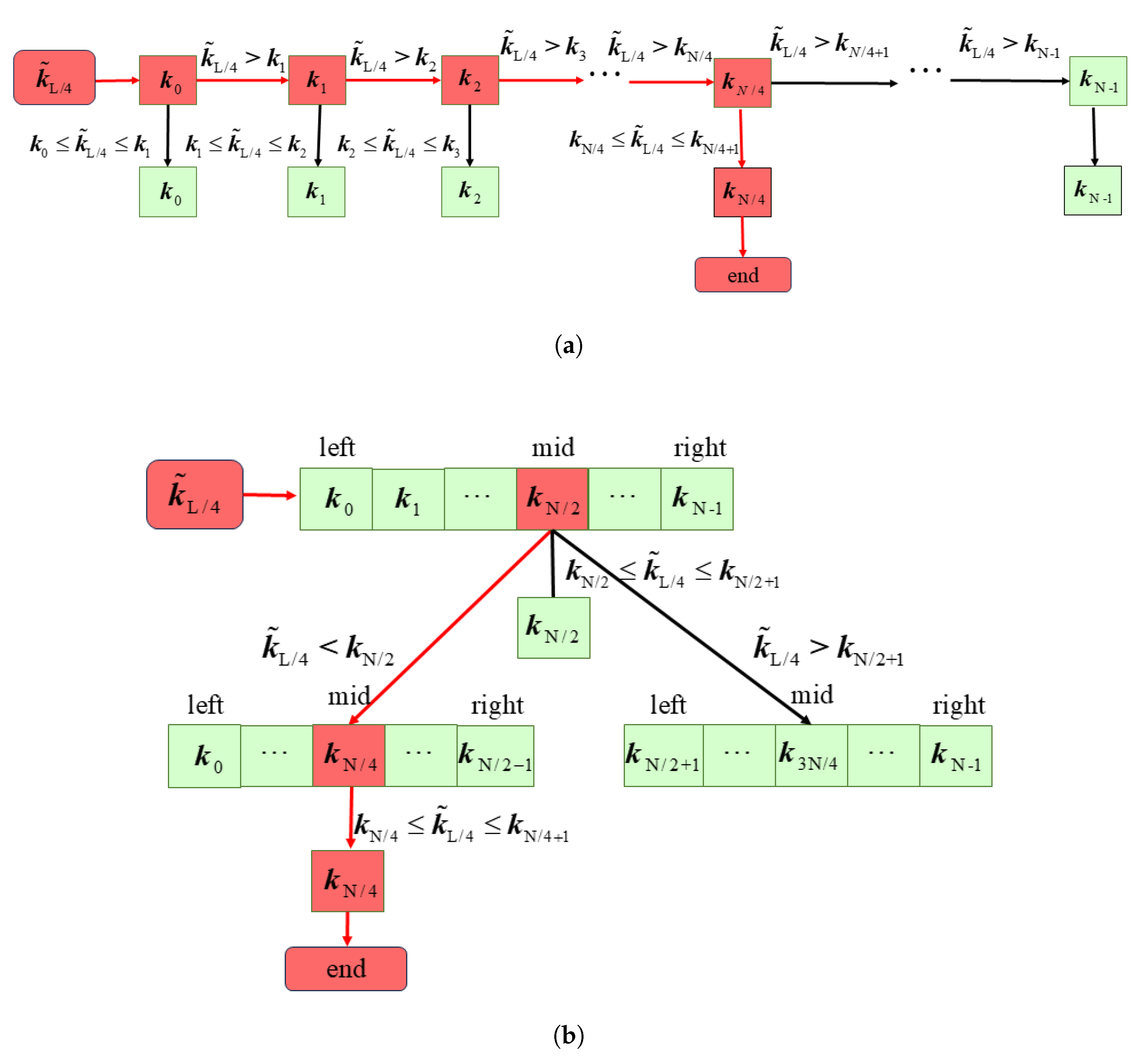
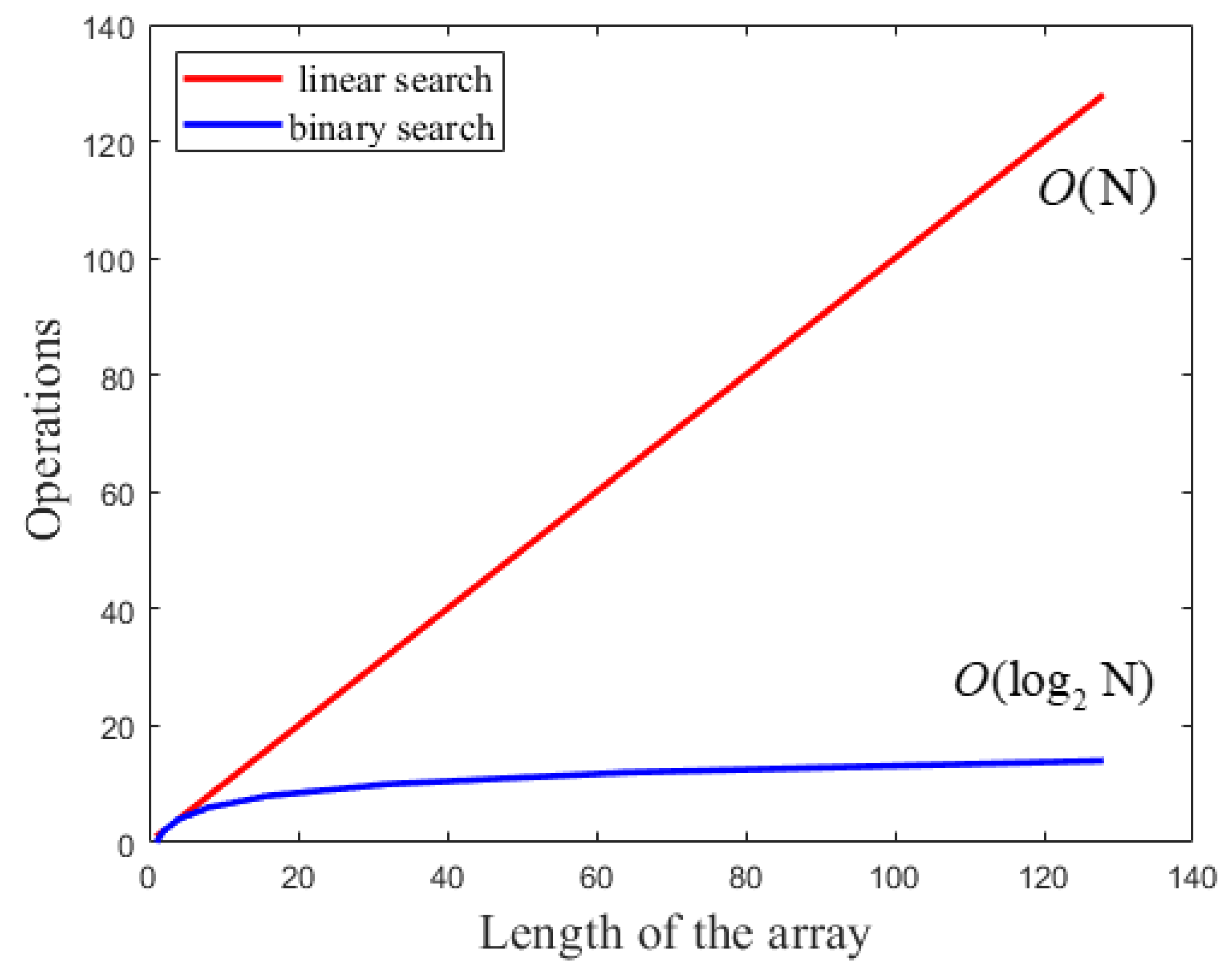
3.3. Two-Dimensional CSG Interpolation
| Algorithm 3: Binary search |
|
4. Experimental Results and Analysis
5. Conclusions
Author Contributions
Funding
Data Availability Statement
Conflicts of Interest
References
- Lorente, D.; Limbach, M.; Gabler, B.; Esteban, H.; Boria, V.E. Sequential 90 Rotation of Dual-polarized Antenna Elements in Linear Phased Arrays with Improved Cross-polarization Level for Airborne Synthetic Aperture Radar Applications. Remote Sens. 2021, 13, 1430. [Google Scholar] [CrossRef]
- Liu, C.A.; Chen, Z.X.; Shao, Y.; Chen, J.S.; Hasi, T.; Pan, H.Z. Research Advances of SAR Remote Sensing for Agriculture Applications: A Review. J. Integr. Agric. 2019, 18, 506–525. [Google Scholar] [CrossRef]
- Gao, J.; Deng, B.; Qin, Y.; Wang, H.; Li, X. An Efficient Algorithm for MIMO Cylindrical Millimeter-wave Holographic 3-D Imaging. IEEE Trans. Microw. Theory Tech. 2018, 66, 5065–5074. [Google Scholar] [CrossRef]
- Sheen, D.M.; Jones, A.M.; Hall, T.E. Simulation of Active Cylindrical and Planar Millimeter-wave Imaging Systems. In Proceedings of the Passive and Active Millimeter-Wave Imaging XXI, Orlando, FL, USA, 15–19 April 2018; SPIE: Bellingham, WA USA, 2018; pp. 47–57. [Google Scholar]
- Alibakhshikenari, M.; Virdee, B.S.; Limiti, E. Wideband Planar Array Antenna Based on SCRLH-TL for Airborne Synthetic Aperture Radar Application. J. Electromagn. Waves Appl. 2018, 32, 1586–1599. [Google Scholar] [CrossRef]
- Appleby, R.; Wallace, H.B. Standoff Detection of Weapons and Contraband in the 100 GHz to 1 THz Region. IEEE Trans. Antennas Propag. 2007, 55, 2944–2956. [Google Scholar] [CrossRef]
- Kim, B.; Yoon, K.S.; Kim, H.J. Gpu-accelerated Laplace Equation Model Development Based on CUDA Fortran. Water 2021, 13, 3435. [Google Scholar] [CrossRef]
- Gao, Y.; Han, J.; Tian, H.; Zhang, R.; Zheng, S.; Wang, H. GPU Acceleration Method Based on Range-Doppler Highly Squint Algorithm. In Proceedings of the 2023 4th China International SAR Symposium (CISS), Xi’an, China, 4–6 December 2023; IEEE: New York, NY, USA, 2023; pp. 1–4. [Google Scholar]
- Cui, Z.; Quan, H.; Cao, Z.; Xu, S.; Ding, C.; Wu, J. SAR Target CFAR Detection via GPU Parallel operation. IEEE J. Sel. Top. Appl. Earth Obs. Remote Sens. 2018, 11, 4884–4894. [Google Scholar] [CrossRef]
- Wu, S.; Xu, Z.; Wang, F.; Yang, D.; Guo, G. An Improved Back-projection Algorithm for GNSS-R BSAR Imaging Based on CPU and GPU Platform. Remote Sens. 2021, 13, 2107. [Google Scholar] [CrossRef]
- Yang, T.; Zhang, X.; Xu, Q.; Zhang, S.; Wang, T. An Embedded-GPU-Based Scheme for Real-Time Imaging Processing of Unmanned Aerial Vehicle Borne Video Synthetic Aperture Radar. Remote Sens. 2024, 16, 191. [Google Scholar] [CrossRef]
- Li, Z.; Qiu, X.; Yang, J.; Meng, D.; Huang, L.; Song, S. An Efficient BP Algorithm Based on TSU-ICSI Combined with GPU Parallel Computing. Remote Sens. 2023, 15, 5529. [Google Scholar] [CrossRef]
- Tan, Y.; Huang, H.; Lai, T. Real-Time Imaging Scheme of Short-Track GB-SAR Based on GPU+ OpenMP. IEEE Sens. J. 2024, 25, 4990–5002. [Google Scholar] [CrossRef]
- Gou, L.; Li, Y.; Zhu, D.; Wei, Y. A Real-time Algorithm for Circular Video SAR Imaging Based on GPU. Radar Sci. Technol. 2019, 17, 550–556. [Google Scholar]
- Ren, Z.; Zhu, D. A GPU-Based Two-Step Approach for High Resolution SAR Imaging. In Proceedings of the 2021 IEEE 6th International Conference on Signal and Image Processing (ICSIP), Nanjing, China, 22–24 October 2021; IEEE: New York, NY, USA, 2021; pp. 376–380. [Google Scholar]
- Ding, L.; Dong, Z.; He, H.; Zheng, Q. A Hybrid GPU and CPU Parallel Computing Method to Accelerate Millimeter-Wave Imaging. Electronics 2023, 12, 840. [Google Scholar] [CrossRef]
- Li, J.; Song, L.; Liu, C. The Cubic Trigonometric Automatic Interpolation Spline. IEEE/CAA J. Autom. Sin. 2017, 5, 1136–1141. [Google Scholar] [CrossRef]
- Liu, J.; Qiu, X.; Huang, L.; Ding, C. Curved-path SAR Geolocation Error Analysis Based on BP Algorithm. IEEE Access 2019, 7, 20337–20345. [Google Scholar] [CrossRef]
- Wang, G.; Qi, F.; Liu, Z.; Liu, C.; Xing, C.; Ning, W. Comparison between Back Projection Algorithm and Range Migration Algorithm in Terahertz Imaging. IEEE Access 2020, 8, 18772–18777. [Google Scholar] [CrossRef]
- Miao, X.; Shan, Y. SAR Target Recognition via Sparse Representation of Multi-view SAR Images with Correlation Analysis. J. Electromagn. Waves Appl. 2019, 33, 897–910. [Google Scholar] [CrossRef]
- Ding, L.; He, H.; Wang, T.; Chu, D. Cylindrical SAR Imaging Based on a Concentric-square-grid Interpolation Method. J. Electron. Inf. Technol. 2024, 46, 249–257. [Google Scholar]
- Soumekh, M. Reconnaissance with Slant Plane Circular SAR Imaging. IEEE Trans. Image Process. 1996, 5, 1252–1265. [Google Scholar] [CrossRef]
- Xueming, P.; Wen, H.; Yanping, W.; Kuoye, H.; Yirong, W. Downward Looking Linear Array 3D SAR Sparse Imaging with Wave-front Curvature Compensation. In Proceedings of the 2013 IEEE International Conference on Signal Processing, Communication and Computing (ICSPCC 2013), Kunming, China, 5–8 August 2013; IEEE: New York, NY, USA, 2013; pp. 1–4. [Google Scholar]
- Berland, F.; Fromenteze, T.; Decroze, C.; Kpre, E.L.; Boudesocque, D.; Pateloup, V.; Di Bin, P.; Aupetit-Berthelemot, C. Cylindrical MIMO-SAR Imaging and Associated 3-D Fourier Processing. IEEE Open J. Antennas Propag. 2021, 3, 196–205. [Google Scholar] [CrossRef]
- Xin, W.; Lu, Z.; Weihua, G.; Pcng, F. Active Millimeter-wave Near-field Cylindrical Scanning Three-dimensional Imaging System. In Proceedings of the 2018 International Conference on Microwave and Millimeter Wave Technology (ICMMT), Chengdu, China, 7–11 May 2018; IEEE: New York, NY, USA, 2018; pp. 1–3. [Google Scholar]
- Yang, T.; Xu, Q.; Meng, F.; Zhang, S. Distributed Real-time Image Processing of Formation Flying SAR Based on Embedded GPUs. IEEE J. Sel. Top. Appl. Earth Obs. Remote Sens. 2022, 15, 6495–6505. [Google Scholar] [CrossRef]
- Tian, H.; Hua, W.; Gao, Y.; Sun, Z.; Cai, M.; Guo, Y. Research on Real-time Imaging Method of Airborne SAR Based on Embedded GPU. In Proceedings of the 2022 3rd China International SAR Symposium (CISS), Shanghai, China, 2–4 November 2022; IEEE: New York, NY, USA, 2022; pp. 1–4. [Google Scholar]
- Lin, A. Binary search algorithm. WikiJournal Sci. 2019, 2, 1–13. [Google Scholar] [CrossRef]
- Bajwa, M.S.; Agarwal, A.P.; Manchanda, S. Ternary search algorithm: Improvement of Binary Search. In Proceedings of the 2015 2nd International Conference on Computing for Sustainable Global Development (INDIACom), New Delhi, India, 11–13 March 2015; IEEE: New York, NY, USA, 2015; pp. 1723–1725. [Google Scholar]


| Parameter | Parameter Symbol | Value |
|---|---|---|
| Working frequency range | f | 30–35 GHz |
| Frequency-dimension points | 100 | |
| Angle-dimension points | 1440 | |
| Height-dimension points | 128 | |
| Frequency-dimension sampling interval | 50 MHz | |
| Angle-dimension sampling interval | ||
| Height-dimension sampling interval | 0.005 m |
| Method | FT | Phase Compensation | 2D Interpolation |
|---|---|---|---|
| The CPU implementation | FFTW | / | CSG method |
| The conventional GPU implementation | cuFFT | global memory | traversal method |
| The proposed GPU implementation | cuFFT | shared memory | CSG method + partitioning parallel processing |
| Dimension | Metrics | Method | |
|---|---|---|---|
| CPU Implementation | GPU Implementation | ||
| Azimuth dimension | PSLR (dB) | −11.0104 | −11.0071 |
| ISLR (dB) | −10.9234 | −10.9199 | |
| IRW (m) | 0.1662 | 0.1663 | |
| Distance dimension | PSLR (dB) | −12.3573 | −12.3564 |
| ISLR (dB) | −11.0849 | −11.0705 | |
| IRW (m) | 0.0968 | 0.0967 | |
| Height dimension | PSLR (dB) | −11.0305 | −11.0273 |
| ISLR (dB) | −9.9241 | −9.9198 | |
| IRW (m) | 0.1666 | 0.1663 | |
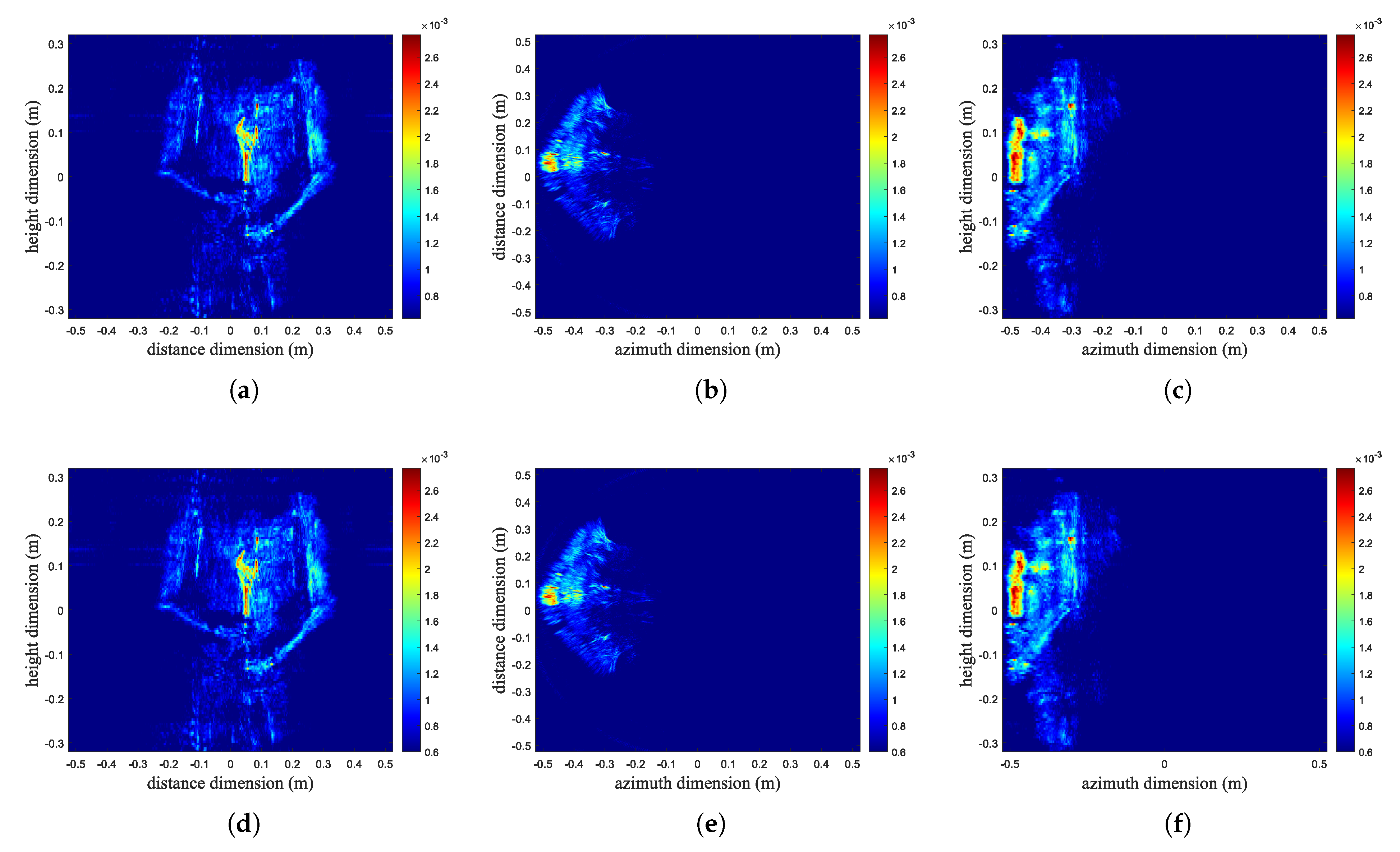
| Value | Front View | Top View | Side View |
|---|---|---|---|
| PSNR (dB) | 37.97 | 37.55 | 38.21 |
| SSIM | 0.909 | 0.922 | 0.914 |
| Optimization Techniques | Time (s) |
|---|---|
| the proposed GPU implementation | 0.794 |
| CSG method + binary search + CUDA stream | 0.821 |
| Shared memory | 4.706 |
| Shared memory + CSG method | 1.737 |
| Shared memory + CSG method + binary search | 1.492 |
| Shared memory + CSG method + CUDA stream | 0.902 |
Disclaimer/Publisher’s Note: The statements, opinions and data contained in all publications are solely those of the individual author(s) and contributor(s) and not of MDPI and/or the editor(s). MDPI and/or the editor(s) disclaim responsibility for any injury to people or property resulting from any ideas, methods, instructions or products referred to in the content. |
© 2025 by the authors. Licensee MDPI, Basel, Switzerland. This article is an open access article distributed under the terms and conditions of the Creative Commons Attribution (CC BY) license (https://creativecommons.org/licenses/by/4.0/).
Share and Cite
Cui, M.; Li, P.; Bu, Z.; Xun, M.; Ding, L. GPU-Optimized Implementation for Accelerating CSAR Imaging. Electronics 2025, 14, 2073. https://doi.org/10.3390/electronics14102073
Cui M, Li P, Bu Z, Xun M, Ding L. GPU-Optimized Implementation for Accelerating CSAR Imaging. Electronics. 2025; 14(10):2073. https://doi.org/10.3390/electronics14102073
Chicago/Turabian StyleCui, Mengting, Ping Li, Zhaohui Bu, Meng Xun, and Li Ding. 2025. "GPU-Optimized Implementation for Accelerating CSAR Imaging" Electronics 14, no. 10: 2073. https://doi.org/10.3390/electronics14102073
APA StyleCui, M., Li, P., Bu, Z., Xun, M., & Ding, L. (2025). GPU-Optimized Implementation for Accelerating CSAR Imaging. Electronics, 14(10), 2073. https://doi.org/10.3390/electronics14102073