1. Introduction
In multivariate time series data, malfunctions or attacks may result in data that significantly deviate from the normal regime, commonly referred to as anomalies. Discovering and flagging these deviations is often defined as multivariate time series (MTS) anomaly detection. Early and accurate detection of anomalies in multivariate time series data is critical for preventing operational disruptions and minimizing economic losses, including ensuring the safety of large-scale systems [
1], detecting cyber-security intrusions [
2], and preventing credit card fraud [
3]. However, anomalies are inherently challenging to identify due to two key factors. First, they stem from rare events, making them sparsely represented in datasets and difficult to annotate comprehensively. Second, defining the entire spectrum of potential anomalous events is typically unfeasible, undermining the validity of supervised learning methods [
4]. Consequently, unsupervised methods, which do not rely on labeled data, have emerged as the preferred approach for detecting MTS anomalies.
Traditional unsupervised techniques, such as linear-based methods [
5], distance-based methods [
6], density-based methods [
7], classification-based methods [
8,
9], and distribution-based methods [
10], often fail to incorporate temporal dependencies and have difficulty with high-dimensional variables, limiting their real-world applicability. Recent advancements in deep learning have introduced reconstruction-based techniques [
11,
12] and prediction-based methods [
13,
14], which leverage errors as indicators of anomalies. However, these methods frequently overlook explicit inter-variable relationships, hindering their ability to fully exploit inherent MTS correlations. Methods using graph neural networks (GNNs), such as the graph deviation network (GDN) [
15] and graph learning with Transformer for anomaly detection (GTA) [
16], address these limitations by capturing both temporal and spatial dependencies between variables, offering improved insights into their behaviors and interactions [
17].
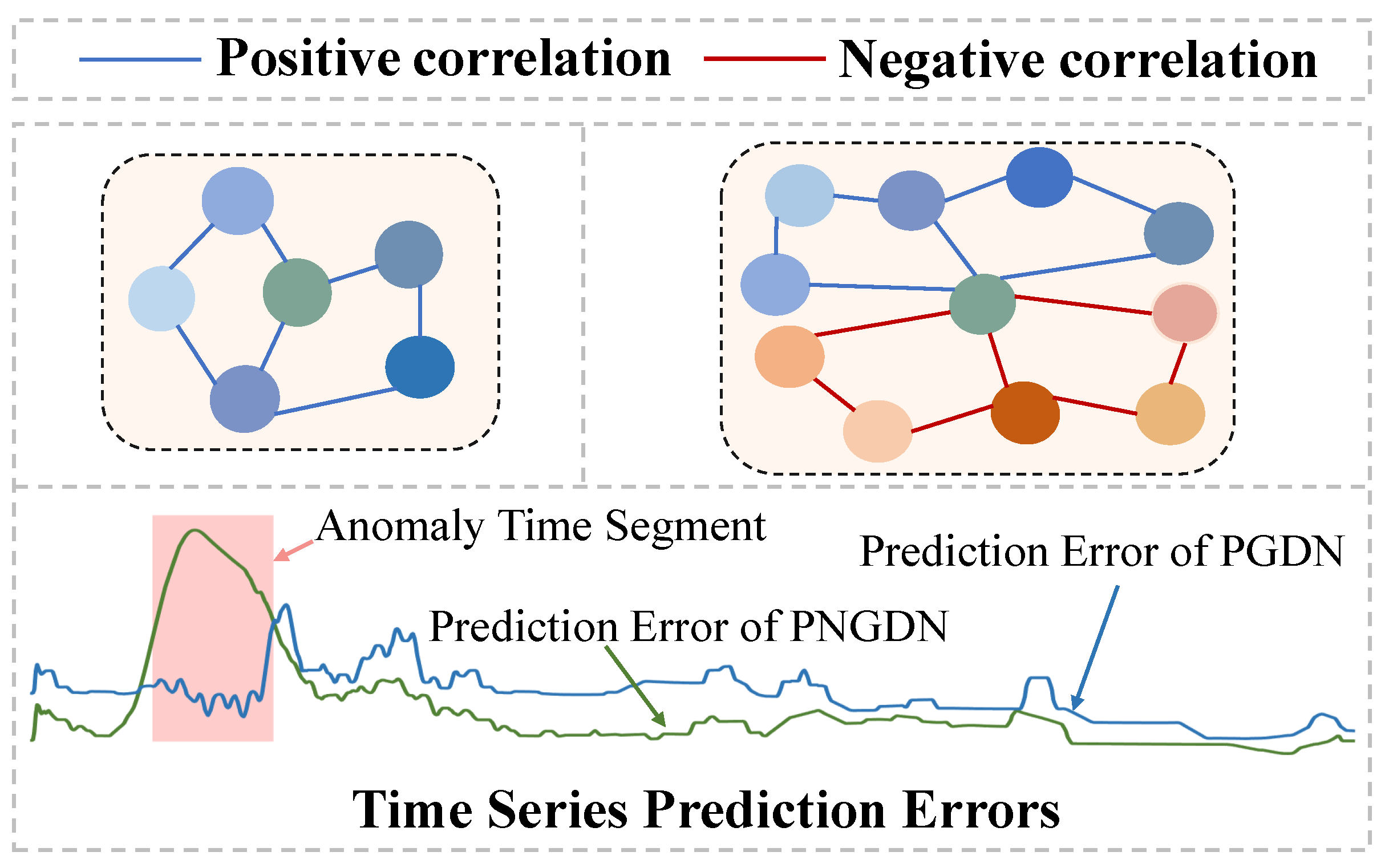
Nevertheless, after carefully analyzing the dataset characteristics in existing studies, we highlight the following challenges in the current application of GNNs for MTS: (1) Inability to handle relational noise: A subset of methods does not filter out relational noise but treats all relationships as a single correlation graph, which hinders the accurate modeling of inter-variable dependencies. (2) Focus on positive correlations only: In MTS, unique patterns in one variable may influence unrelated variables, thereby increasing computational cost. Hence, most existing approaches focus solely on modeling positive correlations between variables, disregarding the critical role of negative correlations. As shown in
Figure 1, by excluding negative correlations, existing GNN-based methods miss important relational features, leading to lower prediction errors during anomalies, reducing anomaly detectability and weakening their effectiveness in complex scenarios.
To tackle the aforementioned challenges, we draw inspiration from CrossGNN, an early attempt to use signed variable correlation graphs in MTS forecasting, and propose the Positive and Negative correlation Graph Deviation Network (PNGDN), which decomposes inter-variable relationships into positive and negative correlation dependencies. These dependencies are modeled separately to capture their respective impacts on the time series, making the method well-suited for anomaly detection in complex scenarios. To better model positive and negative correlations and eliminate relational noise from unrelated variables, the method first utilizes a variable embedding module and an inter-variable correlation graph learning module to extract variable features and construct positive and negative correlation graphs with strong relationships. To address the differences in information propagation across positive and negative neighbors, we further apply an attention-based mechanism to each graph to generate the predicted values for each variable. This design amplifies prediction errors during anomalies and enhances interpretability. Finally, the anomaly detector uses prediction errors to identify anomalies in MTS. Experimental results demonstrate that PNGDN achieves superior performance on real-world datasets. Overall, our contributions are summarized as follows:
Motivated by the observed significance of both positive and negative correlations in time series data, we introduce PNGDN, a novel framework that models these inter-variable relationships comprehensively, mitigating relational noise and enhancing anomaly detection accuracy. This approach addresses the critical limitations of prior methods that rely solely on positive correlations, enabling a more accurate representation of dynamic dependencies.
We design a tailored message-passing strategy based on attention mechanisms, explicitly separating the effects of positive and negative correlations. This innovative approach amplifies prediction errors, significantly enhancing the model’s ability to distinguish anomalies.
Extensive evaluations on three real-world public datasets demonstrate that PNGDN consistently outperforms baseline models in anomaly detection. Furthermore, ablation studies and interpretability analyses further validate its effectiveness and practical applicability.
PNGDN shows strong practical potential for real-world scenarios requiring timely anomaly detection. In cyber–physical systems (CPSs), such as industrial automation and intelligent transportation, it captures complex sensor dependencies to enable accurate detection. Similarly, in environmental monitoring, it detects air quality anomalies by modeling correlations like those between PM2.5 and
or wind speed [
18,
19].
3. Methods
3.1. Problem Definition
In our work, MTS is defined as
and
, which denotes data collected from
N variates over
T time steps. At time step
t, we use a sliding window of size
L and stride
S over historical MTS data to define the model input as
and the target output
, where
and
represent the predictions and observations for all variables at time step
t separately. Concretely, the input
can be expressed as defined in (1):
According to the standard unsupervised MTS anomaly detection framework, the training data are assumed to remain in normal states throughout, and the task objective is to determine whether a given is an anomaly or not.
3.2. Overall Structure
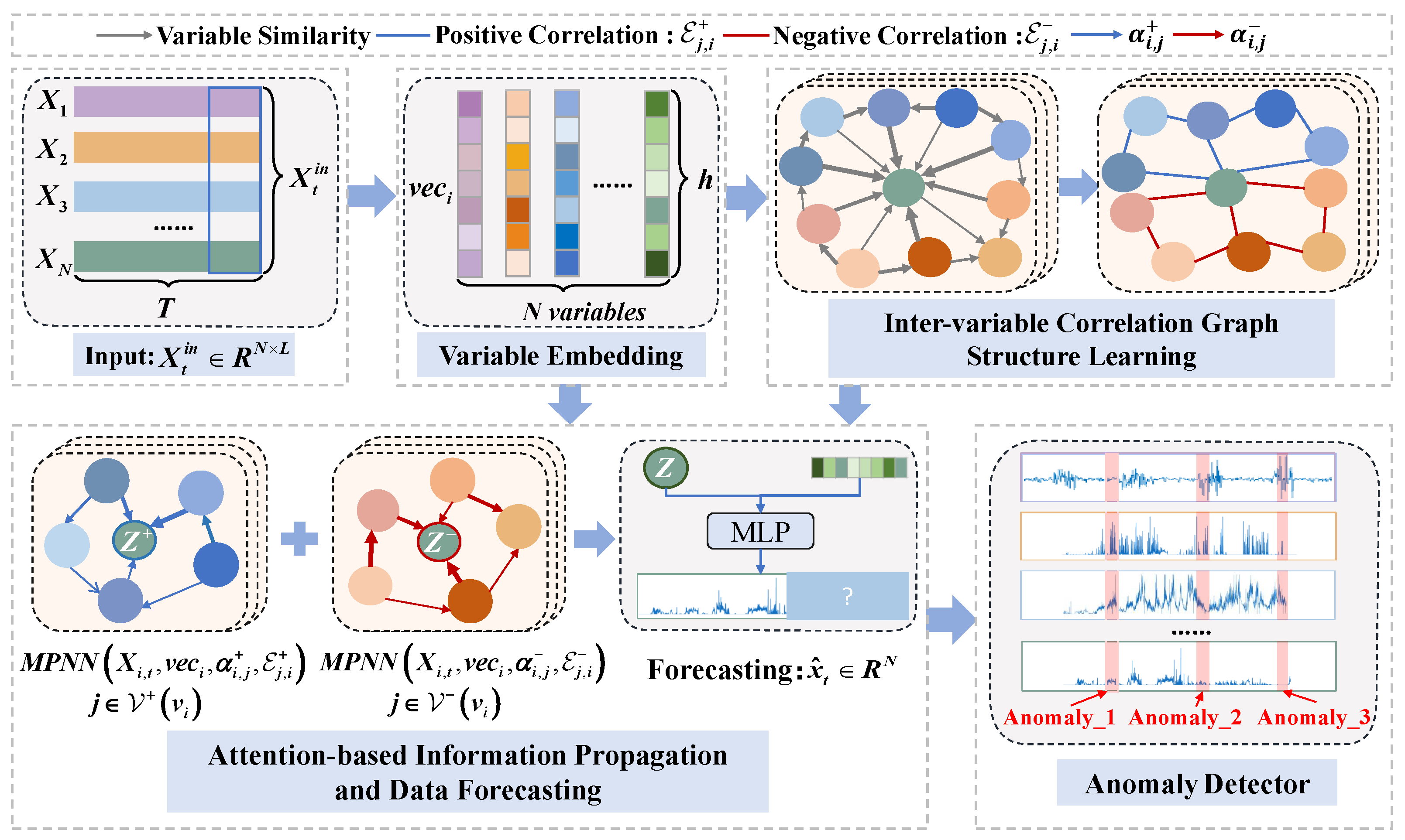
The core idea of our proposed PNGDN model is to effectively leverage the typical positive and negative correlations among time series variables, making the model better suited for complex real-world scenarios. The detailed structure of PNGDN is illustrated in
Figure 2. Specifically, it begins with a variable embedding module to capture each variable’s behaviors and characteristics. Next, the inter-variable correlation graph structure learning module picks strong positive and negative correlations and eliminates relational noise from irrelevant variables, constructing the inter-variable correlation graphs. The attention-based information propagation and data forecasting module is then employed, leveraging graph attention weights to capture the diverse influence of neighboring variables for variable representation and forecasting. Finally, the anomaly detector identifies anomalies by calculating the absolute error between predicted and actual values, thereby identifying the time and variables associated with the anomalies. This approach can amplify prediction errors under anomalous conditions, further enhancing anomaly-detection performance.
3.3. Variable Embedding
In the MTS task, most data originate from different devices that vary simultaneously over time. These variables may exhibit unique but interrelated characteristics. For instance, data measured from identical components of two similar devices tend to exhibit significant positive correlations, while data from components with opposite functions in the same device often show strong negative correlations. To capture these relationships, we introduce a multidimensional embedding vector of size h for each variable to represent its distinct behaviors and characteristics. These variable embeddings, denoted as , are initialized randomly and trained alongside the rest of the model using multivariate data within each sliding window. Through training, the embeddings serve as part of the GNN parameters, enabling the model to better capture variable-specific properties that are otherwise difficult to model through shared GNN weights alone. High absolute values of cosine similarity between embeddings indicate strong variable correlations.
In this model, variable embeddings serve two main purposes: (1) To determine typical dependencies and relational noise among variables and then form the inter-variable correlation graph. (2) To provide variable-specific information to enhance attention-based information propagation and data forecasting, helping the model to distinguish heterogeneous contributions from different neighbors during prediction.
3.4. Inter-Variable Correlation Graph Structure Learning
Most existing studies either focus solely on positive correlations among variables or fail to effectively filter out relational noise in MTS anomaly detection. As a consequence, the deviation between the predicted and actual values during anomalous intervals becomes insufficient, making anomalies harder to distinguish and ultimately degrading detection performance. To address these limitations, this module learns both positive and negative correlations among variables and generates the inter-variable correlation graph . We represent this graph as , where denotes the set of variable nodes, is defined as the i-th variable node, and N is the total number of variables. The edge set refers to , where and denote the edge set with positive correlations and negative correlations, respectively, for variable .
In the process of developing the graph
, we firstly define the candidate correlation set
for variable
as all variables excluding itself, i.e.,
. To determine the dependencies for variable
, the similarity score
is computed between the embedding of node
i and the embeddings of each node in
, which can be formulated as
Then, we choose nodes with
maximum similarity scores as positively correlated neighbors, forming positive correlations, and nodes with
minimum similarity scores as negatively correlated neighbors, forming negative correlations. For variable
, its node sets can be represented as
for positively correlated neighbors and
for negatively correlated neighbors. The values of
and
are determined based on the dataset characteristics and are used to select variable pairs with sufficiently large absolute similarity, ensuring that both strong positive and strong negative correlations are retained while filtering out noisy or irrelevant relationships. This process is formally represented as
where
denotes the directed edges from node
i to node
j, which models the positive correlations from variable
to neighboring variable
as a directed edge. Similarly,
represents the directed edges capturing negative correlations from variable
to neighboring variable
.
3.5. Attention-Based Information Propagation and Data Forecasting
In this paper, we adopt a prediction-based method for anomaly detection in MTS data, assuming low prediction errors during normal periods and higher errors during anomalies. To enhance prediction accuracy and amplify errors for anomalies, we employ an attention-based mechanism to propagate and aggregate positive and negative correlation information based on the inter-variable correlation graph . The resulting representation is then used to predict future data at time step t. The detailed process is described below.
Since the processes of information aggregation and propagation for positive and negative correlations follow the same logic, we take the case of positively correlated neighbors as an example for detailed explanation. We leverage the aforementioned attention-based mechanism as the feature extractor. Considering each variable’s unique properties, we concatenate the variable embedding
with the appropriately transformed historical data
to combine temporal and spatial features simultaneously, which is outlined as follows:
where ⊕ represents concatenation and the subscript
t is disregarded. Then, the resulting combination
is processed together with the learning coefficient
for the attention mechanism, and the attention coefficients are computed by
. These coefficients, denoted as
are then normalized using the
function. The entire process can be represented as
After obtaining the attention coefficients
, we can obtain the positive aggregated representation
for positively correlated neighbors. This can be expressed in the following form:
where
denotes the message-passing neural network for positively correlated neighbors of variable node
.
Hence, for each variable node
,
is defined as the aggregated representation of information for variable node
. The corresponding mathematical expressions are
where
depicts the negative aggregated representation for variable node
.
Subsequently, we acquire the representations of all variables at time step t, denoted as , where the subscript t is omitted for simplicity. However, does not explicitly differentiate the inherent properties of individual variables. To bridge the gap between variable representations and the intrinsic characteristics of each variable, we incorporate variable-specific embeddings into the forecasting process. This allows the network to emphasize or suppress different dimensions in according to each variable’s unique preferences, effectively acting as a soft gating mechanism.
As a result, for each
, the corresponding variable embedding
is element-wise multiplied with
(denoted ∘), and the result serves as input to stacked fully connected layers with input dimension
h and output dimension
N. This layer predicts the values of all variables at time
t, represented as
Finally, we define the mean squared error between the predicted output
and the observed output
for each variable as the loss function, which is formulated as follows:
3.6. Anomaly Detector
For better performance in detecting and interpreting anomalies, we compute individual anomaly scores for each variable and aggregate them into a single anomaly score for each time step, enabling a clearer identification of which variables exhibit anomalies. The anomaly score is determined by comparing the predicted data with the observed true data at time
t, calculating the absolute error for variable
as
. Furthermore, given the varying characteristics of different variables, their anomaly deviations may differ in magnitude. To prevent any single variable’s anomaly deviation from overshadowing others, we normalize the predicted values for each variable. This process is formalized as
where
and
are computed as the median and inter-quartile range of
over the temporal dimension, as these metrics are more robust to anomalies than mean and standard deviation.
To calculate the overall anomaly score
at time
t, our model combines the deviations of all variables through a maximum function, effectively emphasizing the variables displaying anomalies. Also, a simple moving average [
13] is applied to
to smooth the score and mitigate the impact of sharp spikes in normal data.
At last, if
at time step
t surpasses the anomaly threshold, this time step is identified as anomalous. Although techniques like extreme value theory [
28] can be employed to set the threshold, an adaptive threshold is used for simplicity. It is set as the maximum of
in different validation datasets, avoiding the introduction of additional hyperparameters, and aligns better with the real-time, unsupervised nature of MTS anomaly detection tasks.
4. Experiments
4.1. Datasets
We conducted experiments on three real-world publicly available datasets for MTS anomaly detection: Secure Water Treatment (SWaT) [
29], Water Distribution (WADI) [
30], and Server Machine Dataset (SMD) [
31].
The SWaT and WADI datasets are widely used benchmarks in cyber–physical system (CPS) security research; both are provided by operational testbeds simulating real-world water infrastructures. The SWaT dataset originates from a six-stage water treatment system managed by the Singapore Public Utilities Board, incorporating PLCs, EtherNet/IP, and CIP protocols. It provides data collected from 51 sensors, supporting anomaly detection and attack validation studies. In contrast, the WADI dataset is collected from a three-stage water distribution system equipped with extensive pipeline networks and uses the Modbus/TCP protocol. It offers a larger and more complex dataset with 127 sensors, and presents greater modeling challenges due to its higher dimensionality. However, as both systems require 5–6 h to stabilize [
32], we excluded the initial 21,600 unstable data points generated during this period.
The SMD is from a large Internet company, comprising multivariate time series data monitored from 28 server machines over five weeks. Each observation includes 38 metrics such as CPU load, network usage, and memory usage, sampled at one-minute intervals. Designed for entity-level anomaly detection, the SMD captures complex operational behaviors of server machines under real-world conditions, providing a benchmark for evaluating robustness in industrial monitoring scenarios. Given that data from the 28 servers were collected simultaneously, we opted to train and test models for each server individually. The performance metrics are aggregated through averaging validation results across all servers, enabling the selection of the optimal model. This approach ensures robustness and generalizability by tailoring the anomaly detection framework to the operational dynamics of distinct server environments while maintaining statistical reliability.
The statistics of the three datasets are summarized in
Table 1. Due to the high frequency of the original sampling points in the three datasets resulting in large data volumes, we applied downsampling to reduce training time. Concretely, measurements were aggregated at 10-second intervals, with the median value taken as the processed data point. Similarly, the label for each interval was determined as the most frequent label within the 10-second window.
4.2. Baselines
We compare our model, PNGDN, with different baselines representing the main categories of anomaly detection methods: (1) linear-based methods (e.g., PCA [
5]), which project data onto principal components and identify anomalies through deviations in lower-dimensional subspaces; (2) distance-based methods (e.g., KNN [
6]), which calculate distances to the
k nearest neighbors and detect anomalies via aggregated proximity scores; (3) ensemble-based methods (e.g., FB [
33]), which train multiple detectors on random feature subsets to enhance diversity and detect anomalies by aggregating their outlier scores; (4) density-based methods (e.g., DAGMM [
34]), which evaluate the density of time series data to identify anomalies; (5) reconstruction-based methods (e.g., AE [
11], LSTM-VAE [
12], MAD-GAN [
21]), which encode subsequences of normal training time series data in latent space to model normal behavior and detect anomalies based on reconstruction errors; (6) prediction-based models (e.g., M2N2 [
14] and GDN [
15]), which learn predictive models to forecast future variable values from the current context window and identify anomalies using prediction errors.
4.3. Experiment Setup
Our model is implemented using PyTorch version 1.12.1 with CUDA 11.1 [
35] and PyTorch Geometric library version 1.12.1 [
36]. Training is conducted on a server equipped with a 12th Gen Intel(R) Core(TM) i5-12400F 2.50 GHz and a NVIDIA GeForce RTX 2070 GPU. For all three datasets, we use embedding vectors with length of 64 and hidden layers with 128 neurons. At the same time, the value of
is defined as 5 or 30 and
is defined as 5 or 10, respectively, where their values are adjusted based on the number of variables in every dataset. Moreover, the sliding window size is set to five for all datasets. In addition, we choose the Adam optimizer with a learning rate of
for the training of our model. Also, we trained it for a maximum of 30 epochs, with early stopping applied when the performance does not improve for 10 consecutive epochs.
4.4. Performance Comparison and Discussion
We conducted experiments on three real-word datasets to evaluate our model, comparing its performance with the aforementioned eight baseline models in terms of precision (
P), recall (
R), and F1 -score(
F1), area under receiver operating characteristic curve (AUROC,
ROC), and area under the precision-recall curve (AUPRC,
PRC). The first three are calculated as follows:
where TP, TN, FP, and FN are the numbers of true positives, true negatives, false positives, and false negatives, respectively. Higher values across these three metrics indicate better performance. At the same time, the AUROC evaluates model performance across all possible thresholds, reducing sensitivity to any single decision point, while the AUPRC is particularly appropriate for assessing performance under class imbalance [
37,
38], ensuring fairer evaluation. The experimental results are presented in
Table 2.
The results demonstrate that PNGDN achieves the best performance across three real-world datasets: SWaT, WADI, and SMD (except for precision on the WADI dataset). Specifically, on the SWaT dataset, which represents an industrial water treatment system, the F1-score of our model achieves 83%, significantly outperforming M2N2 (78%) and GDN (81%). This highlights PNGDN’s superior ability to capture both inter-variable correlations and temporal dependencies. It also achieves the highest AUROC (88%) and AUPRC (81%) on SWaT, indicating strong and stable anomaly discrimination performance even under class imbalance. On the WADI dataset, which contains higher dimensional data and a lower anomaly ratio (5.82%), PNGDN still maintains an F1-score of 54%, surpassing GDN (51%) and demonstrating robustness in high-dimensional sparse scenarios. In this case, PNGDN again leads with an AUROC of 79% and AUPRC of 49%, showing its ability to generalize under sparse anomaly conditions and to detect rare events with greater precision than GDN (78%/46%) and MAD-GAN (73%/32%). For the SMD, PNGDN obtains an F1-score of 60%, slightly outperforming MAD-GAN (57%), GDN (58%), and M2N2 (57%). Although the performance gap is narrower compared to that in SWaT and WADI, the results still underscore PNGDN’s adaptability to complex IT environments. Additionally, PNGDN achieves a competitive AUROC (86%) and the highest AUPRC (51%) on SMD, further confirming its effectiveness in handling subtle and imbalanced anomalies in large-scale server systems.
The main challenges of the SMD lie in two aspects: First, the presence of 38 metrics (e.g., CPU usage, network traffic) introduces complex interdependencies and noise. Second, most anomalies appear as short-term resource spikes, such as brief CPU peaks. These anomalies are less distinguishable compared to the sustained attacks observed in SWaT or WADI. As a result, they require more fine-grained temporal modeling. It is worth noting that the F1-score, AUROC, and AUPRC ranking across the three datasets (SWaT > SMD > WADI) aligns well with their intrinsic difficulty: SWaT features denser and clearer anomalies, WADI poses the greatest challenge due to its high dimensionality and sparsity, and SMD lies in between due to its heterogeneous metrics and low anomaly salience. These comprehensive results verify the generalizability of PNGDN across diverse and challenging MTS anomaly detection scenarios.
4.5. Ablation Study
We conducted several ablation experiments on the three datasets using modified models of PNGDN by removing specific modules to evaluate the necessity of each component. We mainly investigate the following variants: TOPK+ uses only positive correlation graphs constructed from the top positively correlated neighbors to assess the effectiveness of the negative correlation graph. TOPK-all replaces the dynamic learned graph with a fully connected static graph linking all variables to examine the importance of the learned graph structure. Shared message-passing (SMP) retains the positive and negative correlation graphs but replaces their separate propagation mechanisms with a unified shared propagation mechanism to evaluate the impact of distinct attention-based information propagation. -EMB uses an attention mechanism without variable embeddings to analyze their unique roles in the information propagation and data forecasting process. -ATT disables the attention mechanism entirely, assigning equal weights to all neighbors during information propagation.
The results of the ablation experiments are shown in
Figure 3. The detailed analysis of the results for each modified model is as follows:
TOPK+: As shown in the figure, TOPK+ maintains or slightly improves precision (e.g., 0.99 on SWaT and 0.89 on WADI) but suffers significant recall declines (4.0%, 9.1%, and 5.0% for SWaT, WADI, and SMD, respectively), resulting in overall F1-score reductions of 3.0–4.0%. The AUROC remains strong (0.88 on SWaT, 0.82 on WADI, and 0.85 on SMD), showing that despite the lower recall, TOPK+ still has a good ability to distinguish anomalies. The AUPRC shows a slight drop (0.80 on SWaT, 0.47 on WADI, and 0.46 on SMD), reflecting the impact of recall reductions. This decline in recall can be attributed to TOPK+’s reliance solely on positive correlation graphs, which overlooks negative correlations that may be crucial for modeling time series data, leading to a reduced sensitivity in anomaly detection.
TOPK-all: The static fully connected graph improves precision by 17.0% on WADI (0.86 vs. PNGDN 0.69) but collapses recall by 10.2%, leading to a 5.1% F1-score drop. On SWaT and SMD, both precision and recall degrade (e.g., precision drops 2.0% and 3.1%), with F1-scores declining 5.0% and 4.1%. The AUROC on SWaT drops from 0.88 to 0.86, and on WADI from 0.79 to 0.79, while AUPRC drops from 0.81 to 0.77 on SWaT and 0.45 on WADI. It indicates that the static graph introduces relational noise that hinders the model’s ability to detect anomalies, highlighting the necessity of selectively learning inter-variable dependencies.
SMP: The variant marginally increases WADI precision by 19.0% (0.88 vs. 0.69) but reduces precision on SWaT and SMD by 5.1% and 4.2%. Recall declines sharply across datasets (e.g., 11.0% on WADI), causing F1-score reductions up to 7.1%. The AUROC on SWaT drops from 0.88 to 0.84, and on WADI from 0.79 to 0.76, while AUPRC drops from 0.81 to 0.71 on SWaT and 0.42 on WADI. This indicates that, in the SMP mechanism, information from positive and negative correlations may cancel each other out, leading to the loss of critical information.
-EMB: Removing the variable embeddings from the attention mechanism reduces the average precision by 6.0% (e.g., SWaT: 0.93 vs. 0.99) and recall by 14.0% (e.g., WADI: 0.30 vs. 0.44), resulting in an 8.0–10.1% F1-score declines. The AUROC on SWaT drops from 0.88 to 0.83 and on WADI from 0.79 to 0.74. The AUPRC also decreases from 0.81 to 0.69 on SWaT and from 0.49 to 0.39 on WADI. This demonstrates that variable embeddings are essential to tailor the attention mechanism for the characteristics specific to the individual variable. Without , the model loses its ability to selectively emphasize informative features for each variable, resulting in less effective detecting accuracy.
-ATT: Completely disabling the attention mechanism and assigning equal weights to all neighbors degrades both the precision (e.g., 27.3% drop on SWaT) and recall (e.g., 12.0% drop on WADI), with F1-scores plummeting by up to 15.2%. The AUROC drops from 0.88 to 0.80 on SWaT and from 0.79 to 0.71 on WADI, while the AUPRC decreases from 0.81 to 0.61 on SWaT and from 0.49 to 0.34 on WADI, demonstrating the importance of the attention mechanism for preserving model sensitivity and robustness.
5. Interpretability of Model
To analyze the interpretability of the variable embeddings and the inter-variable correlation graph in the PNGDN model, we make use of the t-SNE method [
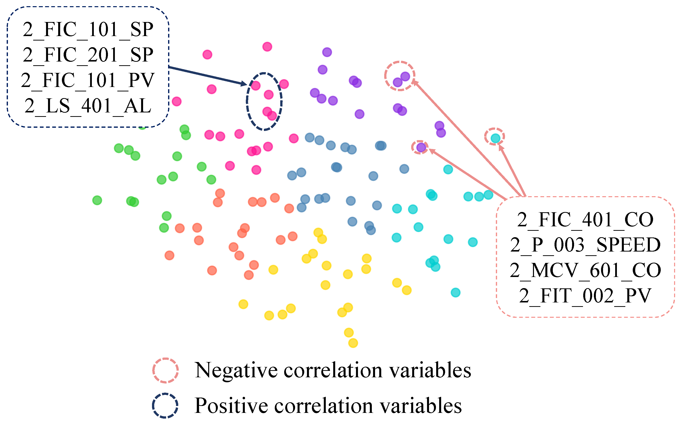
39] and the similarity of our variable embeddings to visualize the variable embeddings. First, to verify whether the variable embeddings effectively reveal behavioral patterns and correlations among variables, t-SNE is utilized to cluster similar variables, making their distributions easier to observe. Secondly, considering that the WADI dataset corresponds to a real-world system with seven distinct sensor categories, the similarity of the variable embeddings is applied to classify the variables. Different colors are assigned to the seven kinds of variables based on the similarities, ensuring that data points belonging to the same category are displayed in the same color, which facilitates the distinction of variable distributions and their correlations. Building on the above conditions,
Figure 4 illustrates the effectiveness of variable embeddings and their roles in the inter-variable correlation graph with practical examples. Detailed interpretations are outlined as follows.
In
Figure 4, variables from the same category cluster together as points of the same color, with positively correlated variables forming uniform-color clusters and negatively correlated variables appearing in different colors and spatially distant from the positive clusters. For example, the dark blue dashed line highlights sensors positively correlated with
, such as
and
, which measure similar metrics in similar water tanks. Conversely, the red dashed line identifies negatively correlated sensors, such as
, which are either located in tanks with opposing functions or measure opposite metrics. These results confirm that variable embeddings effectively reveal variable correlations in inter-variable correlation graphs.
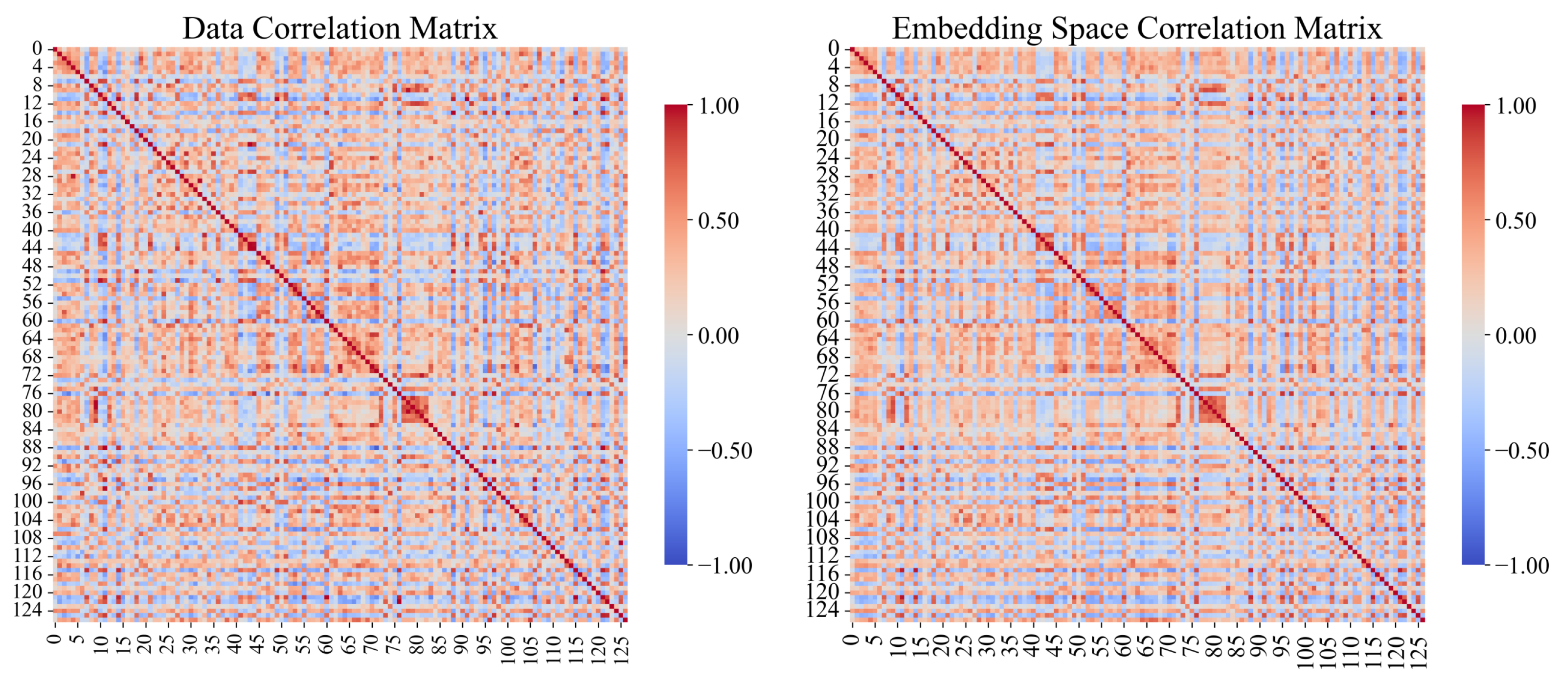
In addition to the qualitative visualization, we further conduct a quantitative analysis to verify whether the variable embeddings preserve real-world dependency structures. Specifically, we compare the cosine similarity matrix derived from the learned variable embeddings with the Pearson correlation coefficient matrix computed directly from the raw MTS data in WADI dataset. As shown in
Figure 5, the two matrices exhibit similar structural patterns despite differences in their absolute similarity magnitudes, indicating that the variable embeddings,
, capture the true statistical correlations among variables. This strongly supports the interpretability and reliability of the variable embeddings for correlation graph construction. At the same time, it should be emphasized that the primary purpose of the variable embeddings is to capture the inherent characteristics of each variable and facilitate the construction of the inter-variable correlation graph. They are not designed to directly reflect or detect real-world anomalies.
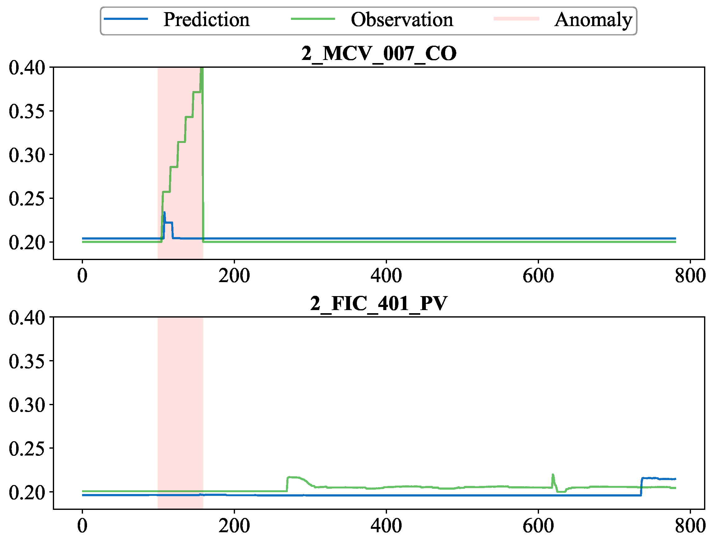
Furthermore, the attention weights in the model, represented as the weights of different edges in the graph, indicate the contribution of various positively and negatively correlated neighbors in modeling variable behavior. To provide a more detailed interpretability analysis of this attention mechanism, we carry out a specific case with a known root cause. As described in the WADI dataset documentation, this anomaly was caused by the malicious activation of the device, leading to water leakage anomalies before water reached consumers.
The model identified the variable
as having the highest anomaly score during this attack, indicating that
was the compromised device. Furthermore, the variable called
, shown in
Figure 6 (below), was detected as the positively correlated neighbor of
with the highest attention weight. By comparing the predicted values and observations of these two variables during the anomalous period in the plot, the anomaly can be further understood. Specifically, for
, its predicted values, influenced by the positive correlation with
, remained at relatively low normal levels for the most part, resulting in a large deviation from the ground truth data.
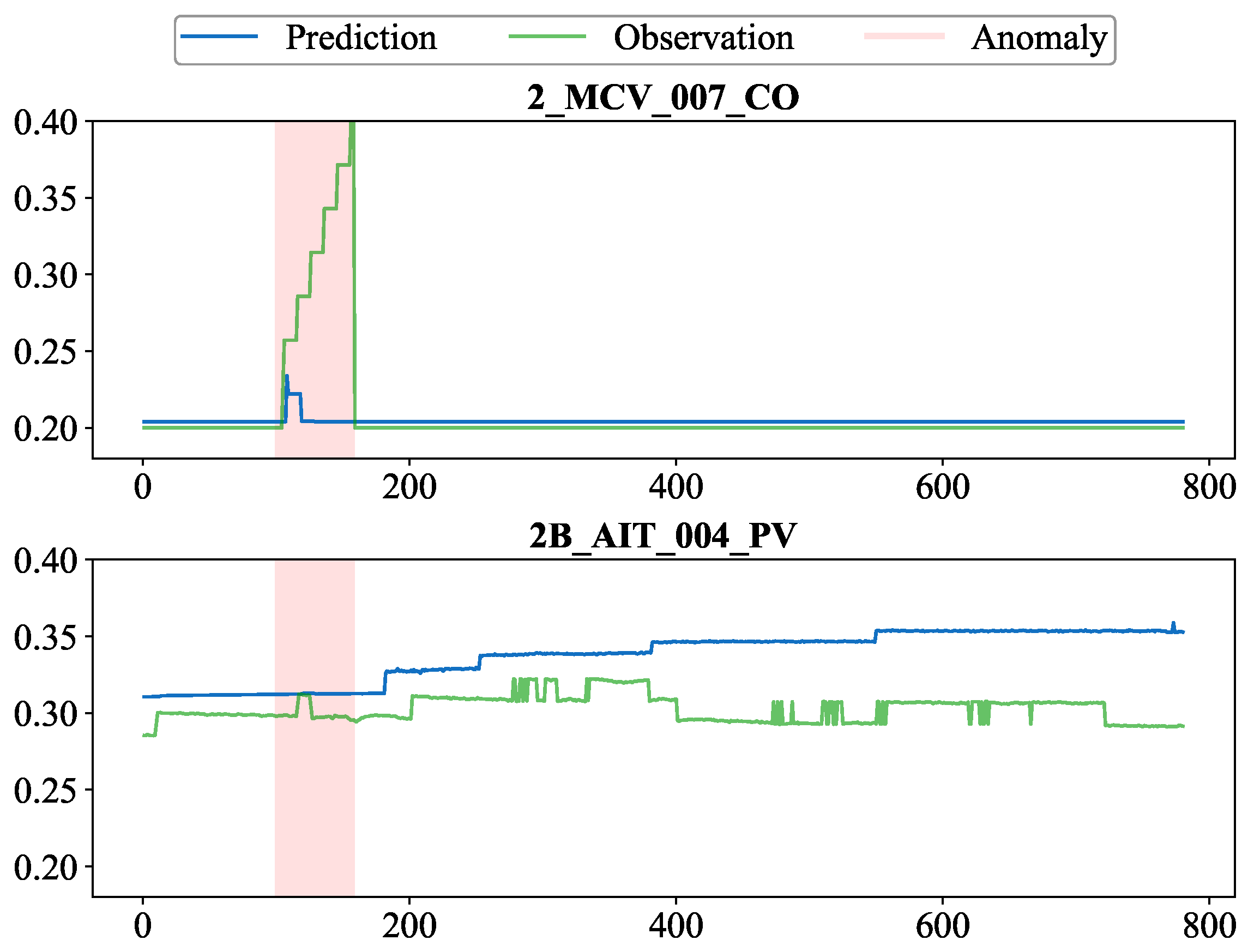
For negatively correlated neighbors of the variable
, the variable with the highest attention weight detected by the model is
. Comparing the predicted and actual values of them within the anomaly time segment shown in
Figure 7 reveals that the negative correlation causes the prediction of
to decrease after a brief increase and then remain at low normal levels. This amplifies the deviation between the true and predicted values of the variable, making the anomaly easier to detect.
Overall, the PNGDN model is capable of detecting anomalies by anomaly scores and influencing the predicted values of variables via correlation relationships and attention weights, thereby amplifying the predicted deviation during anomalies and providing better insight into how the true anomalies deviate from the normal values.
6. Conclusions
This paper proposed PNGDN, a novel multivariate time series anomaly detection model that simultaneously captures positive and negative correlations among variables. By integrating variable embeddings, an inter-variable correlation graph learning module, and an innovative attention-based information propagation mechanism, PNGDN overcomes the limitations of previous methods that relied solely on positive correlations. This dual-correlation approach not only enhances anomaly-detection performance but also improves interpretability by distinctly modeling the contributions of both positive and negative dependencies. To the best of our knowledge, this is the first time negative inter-variable correlations have been explicitly incorporated into GNN-based time series anomaly detection, enabling richer structural understanding and more robust decision-making.
Extensive experiments demonstrate that PNGDN consistently outperforms traditional methods and prior GNN-based models, establishing it as a robust solution for detecting anomalies in complex real-world scenarios. In practical terms, incorporating negatively correlated variables can amplify prediction errors when anomalies occur, further improving detection sensitivity. Also, by using the adaptive threshold strategy, the results of the AUROC and AUPRC confirms that the performance of our model is not affected by the distribution between train and test dataset and aligns better with the unsupervised nature of MTS anomaly detection tasks. Therefore, PNGDN holds strong potential for real-time monitoring in CPS such as water treatment, smart grids, and manufacturing, where data come from diverse sensors and the early detection of abnormal behaviors is essential for system reliability and safety. Specifically, in environmental monitoring, PNGDN identifies air quality anomalies by capturing intricate interactions among pollutants and weather factors, even when the relationships vary in direction. Also, in financial systems, such as credit card fraud detection, PNGDN can identify anomalous transactions by modeling complex correlations among user behavior features, including transaction amount, frequency, location, and device consistency. In the future, PNGDN may be used in more and more time series anomaly detection scenarios to help detect problems early and improve the reliability of important systems.


