Article

Power Prediction Based on Signal Decomposition and Differentiated Processing with Multi-Level Features

1
School of Computer Science and Technology, Zhejiang Sci-Tech University, Hangzhou 310018, China
2
Department of Data Science, New Jersey Institute of Technology, Newark, NJ 07102, USA
*
Authors to whom correspondence should be addressed.
Electronics 2025, 14(10), 2036; https://doi.org/10.3390/electronics14102036
Submission received: 18 April 2025 / Revised: 14 May 2025 / Accepted: 15 May 2025 / Published: 16 May 2025

Abstract

:
As global energy demand continues to rise, accurate load forecasting has become increasingly crucial for power system operations. This study proposes a novel Complete Ensemble Empirical Mode Decomposition with Adaptive Noise-Fast Fourier Transform-inverted Transformer-Long Short-Term Memory (CEEMDAN-FFT-iTransformer-LSTM) methodological framework to address the challenges of component complexity and transient fluctuations in power load sequences. The framework initiates with CEEMDAN-based signal decomposition, which dissects the original load sequence into multiple intrinsic mode functions (IMFs) characterized by different temporal scales and frequencies, enabling differentiated processing of heterogeneous signal components. A subsequent application of Fast Fourier Transform (FFT) extracts discriminative frequency-domain features, thereby enriching the feature space with spectral information. The architecture employs an iTransformer module with multi-head self-attention mechanisms to capture high-frequency patterns in the most volatile IMFs, while a gated recurrent unit (LSTM) specializes in modeling low-frequency components with longer temporal dependencies. Experimental results demonstrate the proposed framework achieves superior performance with an average 80% improvement in R-squared ( R 2 ), 40.1% lower Mean Absolute Error (MAE), and 54.1% reduced Mean Squared Error (RMSE) compared to other models. This advancement provides a robust computational tool for power grid operators, enabling optimal resource dispatch through enhanced prediction accuracy to reduce operational costs. The demonstrated capability to resolve multi-scale temporal dynamics suggests potential extensions to other forecasting tasks in energy systems involving complex temporal patterns.

1. Introduction

The escalating global energy demand driven by economic expansion and urbanization has positioned energy sustainability as a paramount challenge in the 21st-century infrastructure development. Within power systems, the compound annual growth rate (CAGR) of global electricity consumption reached 3.1% during 2000–2021, exerting unprecedented pressure on grid stability and resource adequacy. The International Energy Agency (IEA) reports an 80% aggregate demand growth during this period, with projections indicating a sustained 2% annual increase through 2040 [1]. Emerging economies exhibit particularly dramatic trajectories, evidenced by China’s 300% and India’s 400% consumption surges since 2000, collectively accounting for 63% of global demand growth [2]. This exponential growth pattern necessitates fundamental innovations in power system analytics.
The smart grid paradigm, enabled by synergistic integration of information and communication technologies (ICT) [3] and cyber-physical control systems [4] has revolutionized energy forecasting through three key capabilities: (1) real-time phasor measurement unit (PMU) data acquisition, (2) adaptive demand-response mechanisms, and (3) distributed renewable energy integration [5]. Modern forecasting thus transcends conventional load prediction, emerging as an indispensable component for market-based resource allocation [6], virtual power plant coordination, and transient stability maintenance. However, the operational requirements for forecasting in smart grids, particularly, sub-minute response time and 99.5% prediction accuracy, demand radical improvements in computational efficiency and model robustness.
With the widespread use of smart meters and sensor technologies, the volume of electricity data has grown explosively, exhibiting significant nonlinearity, long-term dependence, and multidimensional interactions [7]. Traditional statistical methods are often unable to provide the necessary flexibility and predictive accuracy to handle these complex features. Moreover, the intermittency and randomness of renewable energy further increase the uncertainty in supply-demand forecasting, requiring models to account for external factors such as weather changes, policy regulations, and market fluctuations [8]. This not only raises higher demands for the flexibility and robustness of algorithms but also necessitates models capable of processing large-scale data quickly and producing high-quality predictions in real-time [9].
In addressing these challenges, machine learning and deep learning methods have garnered widespread attention due to their excellent performance in high-dimensional data analysis. Compared with traditional statistical methods, these approaches can more accurately capture the deep features in complex data through nonlinear mapping and data-driven methods. Recent studies demonstrate that hybrid models combining signal decomposition with deep learning achieve superior performance over single-model architectures. For instance, Li et al. [10] integrated CEEMDAN with LSTM for ultra-short-term load forecasting, yet their framework lacked explicit frequency-domain feature extraction; Li [11] proposed FFT-enhanced LSTM models but failed to address high-frequency transient patterns. These works reveal two critical limitations in existing hybrid approaches: (1) incomplete integration of temporal and spectral features, and (2) uniform processing of heterogeneous signal components regardless of frequency characteristics.
Moreover, the datasets we work with present even greater challenges. On the one hand, electricity data typically only include power consumption values, lacking other useful predictive features; on the other hand, the data volume is relatively small and its features are difficult to extract, making the forecasting task more challenging. To address these issues, building on the previous work, we propose a solution based on the CEEMDAN-FFT-iTransformer-LSTM model. The key innovation of this model lies in its combination of CEEMDAN for signal decomposition, Fast Fourier Transform (FFT), the iTransformer model, and the LSTM model, which are designed to better capture the multi-level features of electricity data. Specifically, CEEMDAN decomposes the original electricity sequence into several intrinsic mode functions (IMFs) with different frequencies, each of which represents distinct signal features. This decomposition allows for more precise handling of each frequency component, thus improving the accuracy of subsequent prediction. The FFT module transforms time-domain signals into frequency-domain signals, enriching the data’s feature representation and helping to capture complex signal patterns. The iTransformer module converts each input feature into an independent token sequence and utilizes multi-head attention mechanisms and feedforward neural networks to enhance its ability to capture global temporal dependencies. Together with the FFT, the iTransformer primarily handles the IMF components with the highest frequency and most rapid changes. Meanwhile, the LSTM module, with its gating mechanism, effectively prevents gradient explosion issues and excels at capturing long-term dependencies, making it particularly suitable for modeling low-frequency, long-term IMF changes. Finally, the entire electricity sequence is forecasted by integrating the predictions from all components. This framework fully leverages the strengths of each component module to build a highly synergistic prediction system.
The main contributions of our work are as follows:
  • Employing Fast Fourier Transform (FFT) to extract frequency-domain features from the data, capturing periodicity and frequency characteristics, thus providing a richer and more accurate feature representation that enhances the model’s understanding of complex signal patterns.
  • Performing CEEMDAN signal decomposition to separate the electricity sequence into different frequency components, each of which is handled separately. This module addresses the complexity of the components in the electricity sequence and provides more precise inputs for subsequent predictions, thereby improving the model’s prediction performance.
  • Integrating iTransformer and LSTM in the feature extraction and prediction process. The iTransformer model focuses on handling high-frequency, rapidly changing IMFs, while the LSTM model addresses low-frequency, long-term IMF changes. By combining these two models, we improve the overall prediction performance, enabling more accurate forecasting of electricity sequences.
The remainder of this paper is organized as follows: Section 2 reviews relevant research in the field of electricity sequence forecasting and analyzes the strengths and weaknesses of existing methods. Section 3 proposes the CEEMDAN-FFT-iTransformer-LSTM framework, detailing the design and implementation of its components. Section 4 describes the experimental datasets and settings, presents the experimental results, and compares our method with other forecasting models, including ablation experiments that analyze the impact of each module on the overall performance. Section 5 concludes our work.

2. Related Work

With the growing demand for refined forecasting in power systems, significant progress has been made in predictive methodologies. Traditional machine learning approaches represented by support vector machines [12] and random forests [13] demonstrated unique advantages in early load forecasting studies due to their strong interpretability and low implementation complexity. However, these methods increasingly reveal limitations in capturing complex patterns when confronting the enhanced nonlinear characteristics and spatiotemporal coupling relationships in modern power data. In this context, nonlinear modeling methods represented by deep neural networks have gained widespread application in load forecasting due to their powerful feature-learning capabilities. For example, Muzaffar’s stacked LSTM [14] demonstrated 0.87 R 2 on German hourly data, outperforming SARIMA by 29 percentage points. And Liu et al. [15] proposed iTransformer, which adopted sparse attention mechanisms and block-wise computation methods, achieving significant improvements in accuracy and efficiency in electricity load and wind power forecasting tasks. Studies have demonstrated that deep learning methods can effectively extract deep data features through multi-layer nonlinear transformations, achieving an average 18% improvement in prediction accuracy over traditional methods when processing high-dimensional time series data [16].
To further enhance predictive performance, the integration of signal decomposition techniques with forecasting models has emerged as a current research focus. Typical decomposition methods include seasonal-trend decomposition (STL) and modal decomposition techniques. Zhu et al. [17] employed STL to decompose load sequences into trend, seasonal, and residual components for separate prediction, effectively reducing mutual interference between components. However, the linear decomposition characteristics struggle to adapt to non-stationary features of power loads, resulting in unresolved mode aliasing in high-frequency components. Addressing this limitation, Li et al. [18] employed wavelet decomposition to process load sequences, utilizing a second-order grey prediction model for individual component forecasting, with final predictions obtained through superposition of component results. Although wavelet decomposition enables effective decomposition of power load data, the selection of basis functions and decomposition levels critically determines predictive outcomes, introducing a priori assumptions that complicate predictive applications. Zhang et al. [19] introduced ensemble empirical mode decomposition (EEMD) to adaptively decompose original sequences into 11 intrinsic mode functions (IMFs), establishing individual prediction models for each component. Experimental results show this approach reduces prediction errors by 23%. The drawback of this method is that EEMD decomposes the load data into 11 subsequences, which greatly increases the computational load of the prediction model.
Current research progress indicates that the field of electricity load forecasting is accelerating towards a “fine-grained decomposition-intelligent fusion” paradigm. It is worth noting that existing methods still face three major challenges: adaptive determination of the decomposition hierarchy, incomplete information mining in high-frequency bands, and computational efficiency optimization in online learning scenarios.

3. The Overall Framework of the Proposed Model for Power Prediction

In this section, we introduce the physical components of the power system and present the overall framework of the proposed model for power demand prediction.

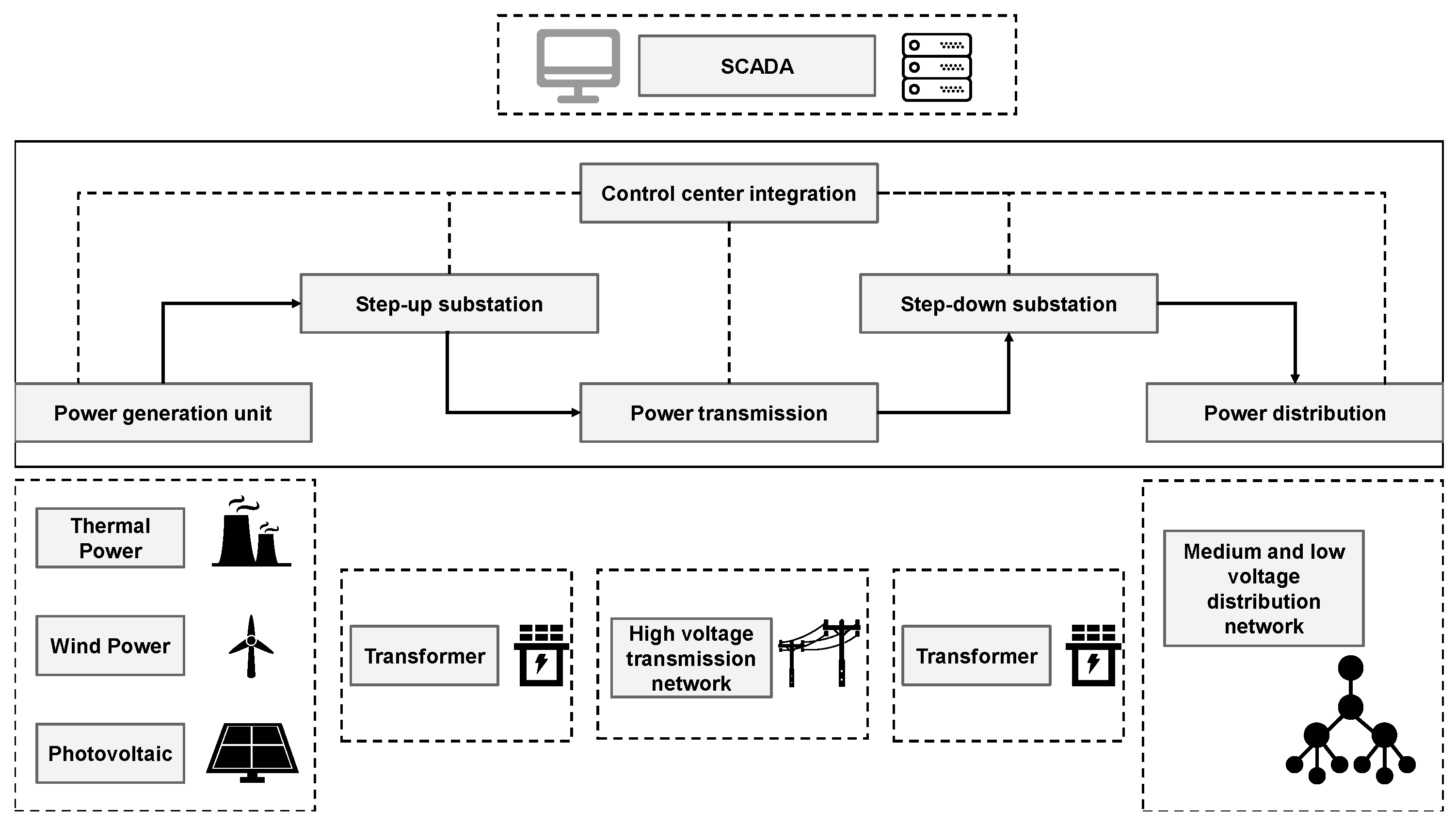
3.1. Power System Components and Sensor Deployment

As shown in Figure 1, the power system consists of four main components: power generation units (e.g., thermal plants, wind farms, and solar farms), transmission networks (including substations and transformers), a general control center, and distribution networks connected to end-users.
The power system begins with electricity generation, where the voltage is increased via step-up substations to facilitate long-distance transmission. High-voltage transmission lines then transport electrical energy from power plants to load centers. Upon reaching the load centers, step-down substations reduce the voltage to levels suitable for consumer use. The stepped-down electricity subsequently enters the distribution network and is ultimately delivered to end-users.
Numerous sensors exist throughout this system. Within power plants, temperature sensors, pressure sensors, and flow sensors monitor equipment operating conditions, ensuring safe and stable production processes while alerting to potential faults. Electrical measurement devices such as voltage transformers and current transformers are installed in both step-up and step-down substations, enabling precise measurement of electrical parameters to guarantee transmission safety and efficiency. Smart meters and other types of sensors deployed at consumer endpoints collect granular electricity consumption data, supporting demand response and load management strategies.
The aforementioned hierarchical sensor deployment ensures comprehensive collection of multi-scale power data: smart meters at the user side capture load detail variations (high-frequency), PMU monitoring systems in transmission networks monitor system-level fluctuations (medium-frequency), and sensors at the generation side track supply-side disturbances (low-frequency). Through comprehensive analysis of sensor data from all system components, the central control center can conduct load forecasting. Specifically, the central control center predicts the electricity demand for the coming week in advance. Based on this forecast, it dynamically adjusts the power generation plan. While ensuring power quality, it effectively avoids the common risk of supply-demand mismatch in traditional power dispatching. This achieves precise coordinated control between power generation and consumption.

3.2. Problem Description

Load forecasting for municipal small-to-medium-sized power grids is a critical task in power system management and is fundamentally a time series prediction problem. A common approach is to employ a rolling window method to generate a new time series X = { X 1 , X 2 , , X N } based on a fixed-length window of size L, where each time point X i represents the observational data collected from day i L to day i. By modeling these time windows, the objective is to generate a corresponding set of forecast sequences Y = { Y 1 , Y 2 , , Y N } , with each Y i defined as Y i = { Y i 1 , Y i 2 , , Y i T } , which contains the forecasted values from day i through day i + T . In the context of our current study, the parameter T is set to 1.

3.3. Overview of Our Structure

In this paper, we propose an integrated forecasting method based on CEEMDAN-FFT-iTransformer-LSTM, which combines the strengths of multiple algorithms to improve forecasting accuracy and efficiency. The structure of the proposed model is shown in Figure 2. The following sections provide a detailed description of the model framework and the forecasting procedure.
  • First, the original power sequence data X ( n ) are input and decomposed using the CEEMDAN algorithm, resulting in several intrinsic mode function (IMF) components and a residual. Typically, IMF1 represents the high-frequency components of the signal, while IMF2, IMF3, ⋯, and IMFn represent the mid- and low-frequency components, which correspond to the medium- and long-term trends in the power sequence.
  • Second, a fast Fourier transform (FFT) is applied to the first IMF to extract frequency domain features. These frequency features are transformed into real numbers and combined with time domain features to form a richer feature space. This step facilitates the capture of the periodic and frequency characteristics of the signal.
  • The frequency and time domain features of IMF1 are then fed into the iTransformer model for forecasting. First, the frequency and time domain features of IMF1 are mapped to a high-dimensional space via an embedding layer, treating each feature as an individual token. Subsequently, a self-attention mechanism processes these tokens to identify and emphasize key features and patterns within the time series. In addition, a feed-forward neural network further refines and processes these features to enhance the model’s understanding of the time series dynamics. Finally, the iTransformer model outputs the forecasted results for IMF1.
  • For the remaining IMF components and the residual, an LSTM is employed for forecasting. Each IMF component is independently input into the LSTM model, which leverages its recurrent structure to memorize past information and predict future values.
  • Finally, the forecasted results of each IMF component and the residual are aggregated through summation to yield the complete forecast for the entire power sequence.

3.4. CEEMDAN

CEEMDAN (Complete Ensemble Empirical Mode Decomposition with Adaptive Noise) is an advanced signal processing technique specifically designed for decomposing non-stationary and nonlinear signals. This component can decompose load curves into physically meaningful components, thus providing strong support for targeted power generation planning. Specifically, when processing a power sequence x ( n ) , the CEEMDAN algorithm [20] introduces Gaussian white noise ϵ i ( n ) over multiple experiments to improve the accuracy of the decomposition. In the i-th experiment, the power sequence can be represented as Equation(1):
x i ( n ) = x ( n ) + ϵ i ( n ) .
The specific steps are as follows:
  • The noise-added sequence X i ( n ) is decomposed using EMD to extract the first-order mode component I M F 1 i ( n ) . By averaging the mode components obtained from N experiments, the IMF of the CEEMDAN decomposition is obtained as Equation (2):
    IMF 1 ( n ) = 1 N i = 1 N IMF 1 i ( n ) .
    The residual after removing I M F 1 ( n ) is then calculated as Equation (3):
    r 1 ( n ) = s ( n ) IMF 1 ( n ) .
  • Gaussian white noise is added to the residual r 1 ( n ) , and the EMD process is repeated to extract the next intrinsic mode function I M F 2 ( n ) and update the residual r 2 ( n ) .
  • This process is continuously repeated until the residual signal exhibits a monotonic trend, at which point the decomposition is terminated. Consequently, the original sequence X ( n ) is decomposed into K sub-sequences along with a residual sequence as Equation (4):
    x ( n ) = k = 1 K IMF k + R ( n ) ,
    where K denotes the total number of intrinsic mode functions obtained, and R ( n ) is the final residual signal.
This method gradually introduces adaptive noise during the signal decomposition process, effectively overcoming the mode mixing issues commonly encountered in traditional Empirical Mode Decomposition (EMD). CEEMDAN not only enhances the accuracy of the decomposition but also addresses the inefficiency in computation. Moreover, by reducing the number of ensemble averages, it minimizes reconstruction errors, thereby yielding more complete and reliable decomposition results.

3.5. Fast Fourier Transformer

Fourier transform is a powerful mathematical tool that can map a signal from the time domain to the frequency domain. This component can be used to extract the high-frequency components of power series in the frequency domain. By combining the frequency domain and time domain, feature extraction becomes easier. Essentially, this technique decomposes a complex waveform into a sum of basic sine waves, revealing the underlying frequency composition of the signal. The Fast Fourier Transform (FFT) [21] is a revolutionary algorithm that greatly improves the computational efficiency of the Discrete Fourier Transform (DFT). When computing the DFT directly, approximately O ( N 2 ) complex multiplications and additions are required, which can lead to a significant computational burden when processing large datasets. The emergence of FFT, by ingeniously exploiting inherent properties, such as the symmetry and periodicity of the signal, has successfully reduced the computational complexity to O ( N l o g N ) , representing a significant advancement.

3.6. iTransformer

This component is responsible for predicting high-frequency components in power sequence forecasting tasks. The core innovation of the iTransformer [22] lies in treating different variables in a time series as independent tokens and capturing the complex dependencies among these variables through a self-attention mechanism. In addition, a feed-forward network is applied to each token to learn its nonlinear representation, thereby enhancing the model’s understanding and forecasting capabilities for time series data. This design enables the iTransformer to effectively handle and predict complex time series data while maintaining computational efficiency.

3.6.1. Embedding Layer

The embedding layer serves to map each time step input x t to a high-dimensional feature vector e t . This mapping is achieved via a linear transformation, mathematically expressed as Equation (5):
E = X W E + b E ,
where E denotes the high-dimensional feature matrix obtained after processing through the embedding layer, with a shape of ( T , d model ) . Here, T represents the length of the time series, and d model denotes the dimension of the embedded vector. X is the original input data matrix with a shape of ( T , d ) , where d indicates the original feature dimension at each time step. W E is the embedding matrix responsible for mapping each feature from the input data to the model’s dimensional space, having a shape of ( d , d model ) . b E is the bias vector, used to adjust each embedded vector, and its shape is ( d model ) .

3.6.2. Multi-Head Self-Attention Mechanism

In the case of complex and redundant power consumption data from industrial users, a single attention mechanism cannot fully capture the information contained in the data. Therefore, the model uses multi-head attention, which allows the model to focus on information from different dimensions from various aspects. After processing through the embedding layer, the data enter the stage of multi-head self-attention. This mechanism maps the input data into multiple subspaces and computes the dot product relationships among queries, keys, and values to capture the complex dependencies between different elements in the input sequence. Each head independently computes its attention weights, and then the outputs from these heads are combined, which significantly enhances the expressive power of the model.
Specifically, the workflow of the multi-head self-attention [23] mechanism is as follows:
  • Query, Key, and Value Mappings: The input data are first mapped into three distinct representations, namely, query, key, and value, using different weight matrices. Assume that there are h attention heads, each with independent linear transformations for queries, keys, and values. For the i-th attention head as Equation (6):
    Q i = X W Q i , K i = X W K i , V i = X W V i ,
    where W Q i , W K i , W V i R d model × d k are the weight matrices for the i-th attention head, d k is the dimension of the query and key, and d m o d e l denotes the model’s dimension.
  • Dot-Product Attention: Each head independently computes the dot product between the queries and keys, scales the result, and then applies the softmax function for normalization to obtain the attention weights as Equation (7):
    W a i = softmax Q i K i T d k ,
    where W a i represents the attention weights.
  • Weighted Sum: The obtained attention weights are used to compute a weighted sum of the values, yielding the self-attention score for each head as Equation (8):
    h e a d i = W a i V i ,
  • Merging the Heads: The outputs from all heads are concatenated to obtain the final output, typically achieved through concatenation followed by a linear transformation as Equation (9):
    H = Concat ( head 1 , head 2 , , head h ) W O ,
    where H R T × ( h · d v ) is the concatenated matrix, and W O R ( h · d v ) × d model is the output linear transformation matrix.

3.6.3. Feed-Forward Network

FFN (Feed-Forward Network) [24] typically consists of two fully connected layers (also known as linear layers) with a nonlinear activation function in between. This structural design enables the FFN to capture complex patterns in the input data and enhance the model’s learning capability through nonlinear transformations. In our model, the structure of the FFN is expressed as Equation (10):
O = R e L U ( X W 1 + b 1 ) W 2 + b 2 ,
where O R T × d model is the final output of the FFN, W 1 R d model × d ff is the weight matrix for the first fully connected layer, b 1 R d ff is the bias vector for the first fully connected layer, W 2 R d ff × d model is the weight matrix for the second fully connected layer, b 2 R d model is the bias vector for the second fully connected layer.
The ReLU activation function in the FFN introduces nonlinearity by converting each input element into a non-negative value. This helps break linear dependencies and enhances the model’s expressive power. This way, the FFN not only effectively transforms the features from the output of the self-attention layer but also further enriches the model’s representational capacity through the nonlinear activation function.

3.6.4. Normalization and Residual Connections

In the iTransformer model, normalization and residual connections are typically used together to achieve more stable and efficient training. The specific application is as follows:
  • Normalization and Residual Connection After the Self-Attention Mechanism as Equation (11):
    Z 1 = LayerNorm ( X + MultiHead ( Q , K , V ) ) ,
    where X is the input, MultiHead ( Q , K , V ) is the output of the self-attention layer, and Z 1 is the output after the normalization and residual connection.
  • Normalization and Residual Connection After the Feed-Forward Network as Equation (12):
    Z 2 = LayerNorm ( Z 1 + FFN ( Z 1 ) ) ,
    where F F N ( Z 1 ) is the output of the feed-forward network, and Z 2 is the final output.
This combined approach not only stabilizes the training process and increases the model’s convergence speed but also enhances the model’s ability to represent complex time series data. In particular, for applications such as power forecasting, the Transformer model, through this method, can more accurately capture both long-term dependencies and short-term variations in the time series, leading to more accurate predictions.

3.7. LSTM

Long Short-Term Memory (LSTM) is a type of Recurrent Neural Network (RNN) designed to address the issue of long-term dependencies, offering significant advantages in handling time series data. This module is mainly designed for predicting medium and low-frequency data in power systems.The architecture of LSTM [25] consists of the input gate, forget gate, output gate, and cell state. The input gate controls whether the model receives new input, the forget gate determines whether to retain previous state information, and the output gate governs whether the model outputs the current state. The cell state, as the core memory unit of the LSTM, stores the network’s state information and is passed across different time steps during the training process.
The computational process of LSTM can be described as follows Equations (13)–(18) [26]:
f t = σ ( W f [ h t 1 , x t ] + b f ) ,
i t = σ ( W i [ h t 1 , x t ] + b i ) ,
C ˜ t = tanh ( W C [ h t 1 , x t ] + b C ) ,
C t = f t C t 1 + i t C ˜ t ,
o t = σ ( W o [ h t 1 , x t ] + b o ) ,
h t = o t tanh ( C t ) ,
where h t 1 represents the output of the LSTM at the previous time step, x t is the input at the current time step, C t 1 is the cell state at the previous time step, and W and b are the weight matrices and bias vectors. The activation values of the input gate, forget gate, and output gate are denoted by i t , f t , and o t , respectively. C ˜ t represents the candidate memory cell state, and the final LSTM output h t is produced by adjusting the current cell state C t through the output gate.
Through these gating mechanisms, LSTM effectively learns and retains long-term dependency information, avoiding the gradient vanishing problem common in traditional RNNs. And in our experiments, we used an LSTM with double hidden layers, which achieved lower error rates in daily electricity consumption prediction compared to single-layer structures [27]. However, it cannot be ignored that under limited training samples, LSTM is prone to overfitting and has weak prediction ability for high-frequency data.

4. Experiments and Performance Evaluation

4.1. Experiment Environment
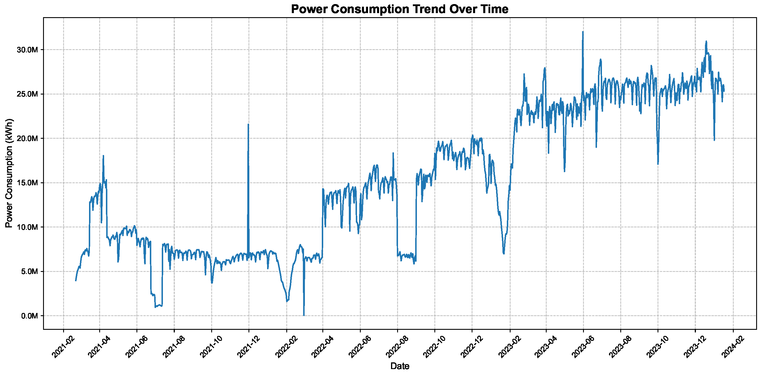
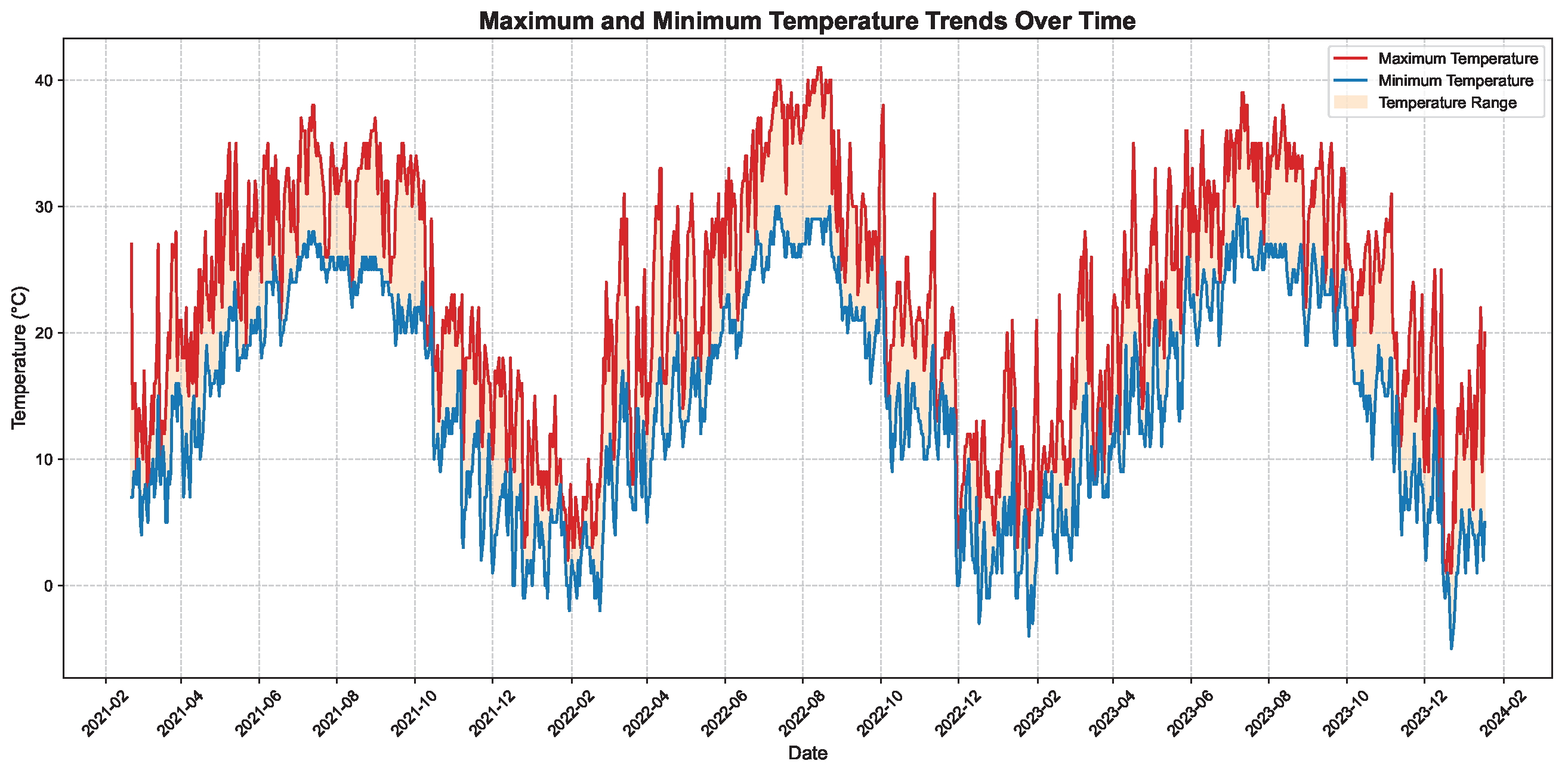
The machine used for the experiments is Legion Y7000 2019 PG0 (Beijing, China), equipped with an NVIDIA GeForce RTX 1650 Ti GPU (Santa Clara, CA, USA) and an Intel(R) Core(TM) i5-9300H CPU @ 2.40 GHz (Santa Clara, CA, USA). The model development environment is based on Python 3.9 and Torch 2.3.0. In all experiments, we conduct 20 repeated trials and report the average experimental results to ensure the reliability of the data and the robustness of the conclusions.

4.2. Dataset

Our dataset comes from the market data of the State Grid Corporation of China (Hangzhou, China), covering daily electricity consumption records in Hangzhou from 2 February 2021, to 17 January 2024. As shown in Figure 3, the data indicate a discernible trend in electricity usage over time. And we collected weather data (including maximum and minimum temperatures) for the corresponding dates to assist with predictions, as shown in Figure 4. Due to the limited dataset size, the data were split into training and testing sets using an 8:2 ratio in the experiment.

4.3. Evaluation Metrics

To comprehensively evaluate the performance of the model, we consider a set of evaluation metrics, including the Mean Absolute Error (MAE), Root Mean Squared Error (RMSE), R-squared ( R 2 ), and Mean Absolute Percentage Error (MAPE), calculated as:
RMSE = 1 n i = 1 n ( Y i Y ^ i ) 2 ,
MAE = 1 n i = 1 n | Y i Y ^ i | ,
MAPE = 100 % n i = 1 n Y i Y ^ i Y i ,
R 2 = 1 i = 1 n ( Y i Y ^ i ) 2 i = 1 n ( Y i Y ¯ ) 2 ,
where n denotes the number of samples, Y i denotes the true value of the i-th sample, Y i ^ denotes the predicted value of the i-th sample by the model, and Y ¯ denotes the average of all actual values of the samples. MAE quantifies the average absolute difference between the predicted and actual values to assess the prediction accuracy in a direction-neutral way, while RMSE amplifies the effect of larger errors by squaring deviations before averaging and taking the square root, thereby emphasising sensitivity to outliers. Meanwhile, MAPE expresses errors as percentages of the actual values to allow scale-invariant comparisons, although its reliability decreases near zero actual values. Finally, R 2 measures the proportion of variance in the dependent variable that is explained by the independent variables, with higher values indicating greater explanatory power of the model.
For Equations (19)–(21), the closer the value is to 0, the smaller the prediction error, indicating higher accuracy. For Equation (22), the value ranges from 0 to 1. The closer the R 2 value is to 1, the stronger the model’s ability to explain the data, demonstrating its effectiveness in capturing the underlying patterns of the data.

4.4. Hyperparameter Selection

To optimize the model performance, we design a series of experiments to choose the best configuration of hyperparameters, sequentially determining the optimal values for lookback_len, epoch, and learning rate.

4.4.1. Lookback_len

First, we determine the lookback_len parameter, which defines how many past days of data are used to predict future outcomes. We choose different fixed time window lengths { 5 , 7 , 9 , 11 , 13 , 15 , 20 , 25 , 30 , 50 } and conduct experiments while keeping the other hyperparameters (learning rate = 0.001, epoch = 50) at their default values. The experimental results, as shown in Figure 5a, show the error values under different lookback window lengths. For ease of observation, we normalize all error values. A 13-day lookback window corresponds to the highest R 2 and the lowest MAPE and RMSE values, suggesting optimal model performance for this configuration. When the lookback window is less than 13 days, the insufficient number of days results in a lack of adequate feature information, leading to suboptimal performance. Conversely, when the lookback window exceeds 13 days, the excessive amount of information renders the model processing redundant, thereby affecting the prediction performance. These results show that a lookback window of 13 days is the optimal choice for this model.

4.4.2. Epochs

The parameter epochs represents the number of training iterations. To investigate its impact on model performance, we choose different numbers of epochs { 10 , 20 , 30 , 40 , 50 , 60 , 70 , 80 } and conduct experiments. The results are shown in Figure 5b. The model achieves its highest R 2 value, lowest RMSE, and smallest MAPE at 30 epochs, suggesting optimal performance for this configuration. When the number of epochs is less than 30, the model is underfitting and fails to fully learn the data features. Conversely, when the number of epochs exceeds 30, the model begins to overfit, leading to a decline in generalization performance. Therefore, having around 30 epochs is the optimal choice for the model.

4.4.3. Learning Rate

The parameter learning rate represents the step size of model updates during each iteration. We choose different learning rates {0.0001, 0.0005, 0.001, 0.005, 0.01} to study their impact on model performance. The experimental results, as shown in Figure 5c, indicate that when the learning rate is 0.0005, the model’s R 2 value reaches its highest, while both RMSE and MAPE are relatively small, suggesting that this learning rate balances convergence speed and model performance. When the learning rate is less than 0.0005, the model’s update steps are too small, leading to slow convergence and suboptimal performance. Conversely, when the learning rate exceeds 0.0005, the update steps become too large, potentially overshooting the optimum or even causing oscillations, which degrades performance. Therefore, using a learning rate of 0.0005 yields the best model performance.

4.4.4. All Hyperparameters

For comprehensive reference, the hyperparameter configuration details are systematically summarized in Table 1:
For medium- and small-scale datasets, the iTransformer architecture was configured with four attention heads, determined through grid search with cross-validation to achieve an optimal balance between multi-scale feature extraction capability and computational efficiency. The embedding layer projects input features into a 128-dimensional latent space, while the feed-forward network dimension adheres to the Transformer design paradigm with d f f = 4 × d m o d e l , enhancing nonlinear representation capacity through intermediate layer expansion. The LSTM architecture employs 128 hidden units to maintain an optimal equilibrium between model capacity and computational overhead, utilizing a two-layer stacked structure to strengthen its ability to model complex temporal dependencies. In the training protocol design, the Adam optimizer was selected over SGD due to its empirically observed 35% faster initial convergence rate and enhanced robustness to learning rate variations. The batch size was maximized within GPU memory constraints to stabilize gradient updates and minimize loss variance. Empirical results indicated that a dropout rate of 0.1 marginally improved test-set R 2 scores by approximately 0.2%, while a higher rate of 0.3 significantly compromised model capacity, reducing effective parameter utilization by 12%. All hyperparameter configurations were rigorously validated against domain-specific benchmarks and experimental performance metrics to ensure reproducibility and generalizability.

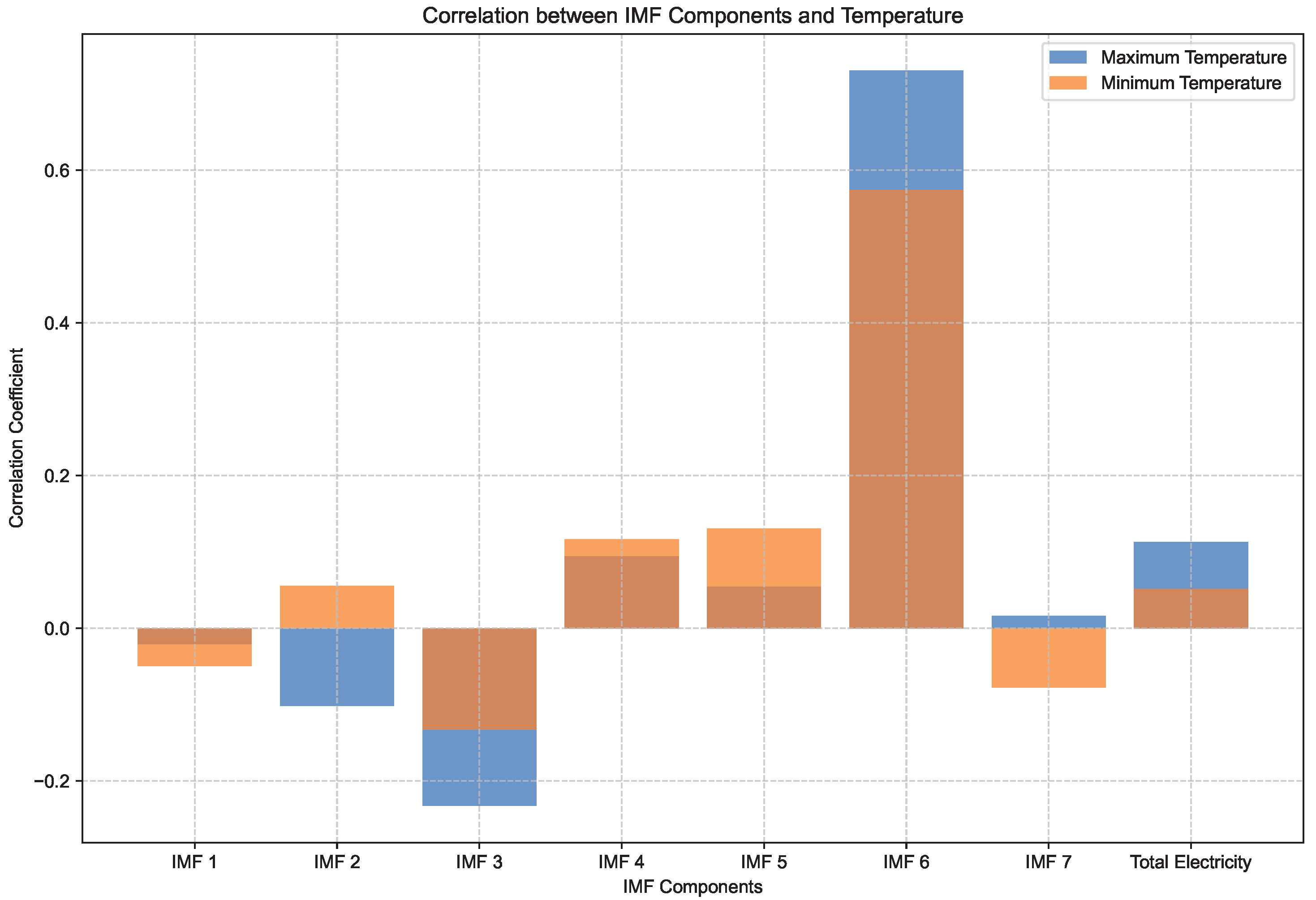
4.5. Analysis of IMFs

Through the CEEMDAN signal decomposition method, the original power load sequence is deconstructed into several physically meaningful intrinsic mode functions (IMFs), and the decomposition results are shown in Figure 6.
From the visual representation of the decomposition results, it can be seen that the initial IMF components (IMF1-IMF3) exhibit significant high-frequency fluctuation characteristics, while the fluctuation frequency of subsequent components (IMF4 and later) gradually becomes smoother. To deeply analyze the temporal characteristics of each IMF component and their coupling relationship with meteorological factors, this study constructed a Pearson correlation coefficient matrix between temperature parameters and each IMF component and the original total power consumption, and the results are visualized in Figure 7.
The correlation analysis results show that the average positive correlation coefficient between the IMF6 component and temperature reaches 0.65, which is a 550% improvement compared to the correlation between the original total power consumption and temperature (0.1), and this feature is particularly prominent in the component set. Based on this feature discovery, when building the prediction model for the IMF6 component, the temperature parameter is innovatively incorporated as a dynamic collaborative feature into the prediction system, and this feature engineering strategy effectively improves the interpretability and prediction accuracy of subsequent prediction models.

4.6. Experiments on the Electricity Dataset

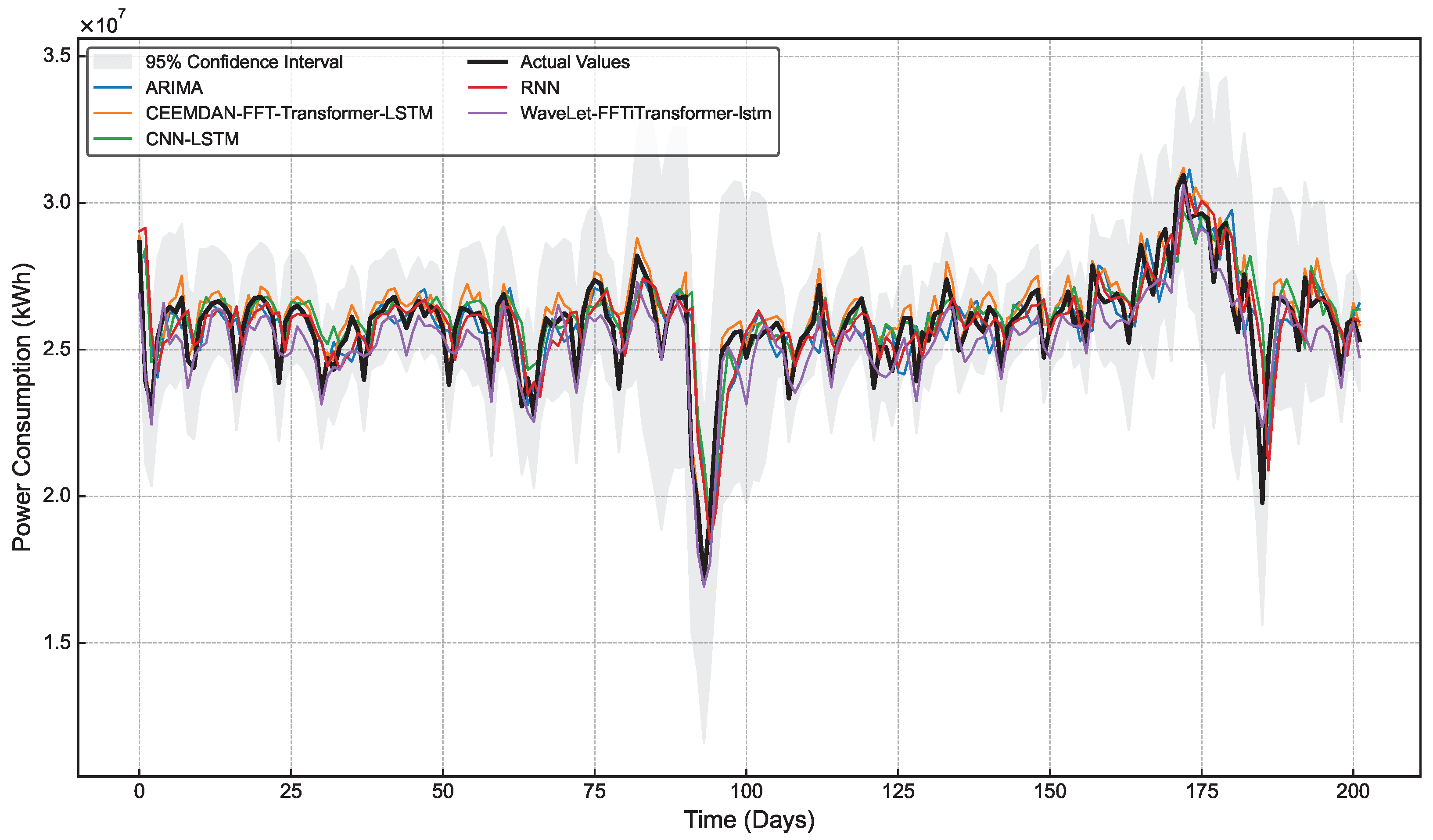
4.6.1. Comparison of Different Models

To validate the superiority of our proposed method, we conduct comparative experiments using MAE, RMSE, R 2 , and MAPE as evaluation metrics, comparing our approach with traditional models, modern models, and composite models. The experimental results are presented in Table 2 and Figure 8. In the comparative analysis among ARIMA, RNN, CNN-LSTM models and Wavelet-FFTiTransformer-lstm, a higher R 2 indicates a better model fit, while lower MAE, RMSE, and MAPE values reflect higher prediction accuracy.
The experimental results show that the ARIMA [28] model performs the worst, with an R 2 value of only 0.4082 and relatively large MAE and RMSE values. This indicates that, as a traditional model, ARIMA exhibits weak predictive capability when processing modern electricity data, struggling to capture the complex patterns and long-term dependencies inherent in the data. Compared with ARIMA, both the RNN [29] and CNN-LSTM [30] models show improved performance. In particular, with the CNN-LSTM composite model, the CNN’s convolutional layers can be used to perform multi-scale decomposition of input sequences, thereby facilitating better feature extraction. So, it achieves a significant reduction in MAE. Notably, the prediction performance after wavelet transform [31] significantly improved compared to the previous two models, but the accuracy is still insufficient. However, despite these improvements in prediction accuracy, neither of these models reaches the desired performance level, indicating that they still have certain limitations in handling more complex electricity consumption forecasting tasks.
In contrast, the CEEMDAN-FFT-iTransformer-LSTM model significantly outperforms the other models on all evaluation metrics, demonstrating exceptional performance. This model achieves an R 2 value as high as 0.9055, far surpassing the other models, which indicates its outstanding model-fitting capability. However, when examining the overall forecast, the model performs poorly in certain sections with lower peak mutations (such as days 90 and 182). This may be due to sudden drops in electricity consumption caused by specific incidents, which disrupted the original daily periodic patterns. But in most cases, its superior performance in terms of MAE, RMSE, and MAPE demonstrates that the model can provide more precise results in predicting electricity consumption data in terms of both identifying outliers and capturing overall trends. Although this model has higher computational complexity, resulting in a single inference time of 691.21 seconds, its improvement in prediction accuracy significantly outweighs the increase in computational cost. Compared to the suboptimal model, our framework achieves a 50.4% reduction in MAE and a 50% improvement in MAPE on daily-granularity data, with only a 38% increase in computation time. This demonstrates that a moderate increase in model complexity can bring significant performance gains in daily prediction scenarios. It is worth noting that daily load forecasting in power systems typically allows for several minutes of computational latency (according to NERC standards [32]), and our model’s real-time performance fully meets practical business requirements. These results fully confirm the strong ability of the CEEMDAN-FFT-iTransformer-LSTM model to capture multi-scale features and complex temporal patterns in electricity consumption data, significantly enhancing both the accuracy and stability of electricity consumption forecasting, and thereby establishing its leading position in electricity time series forecasting tasks.

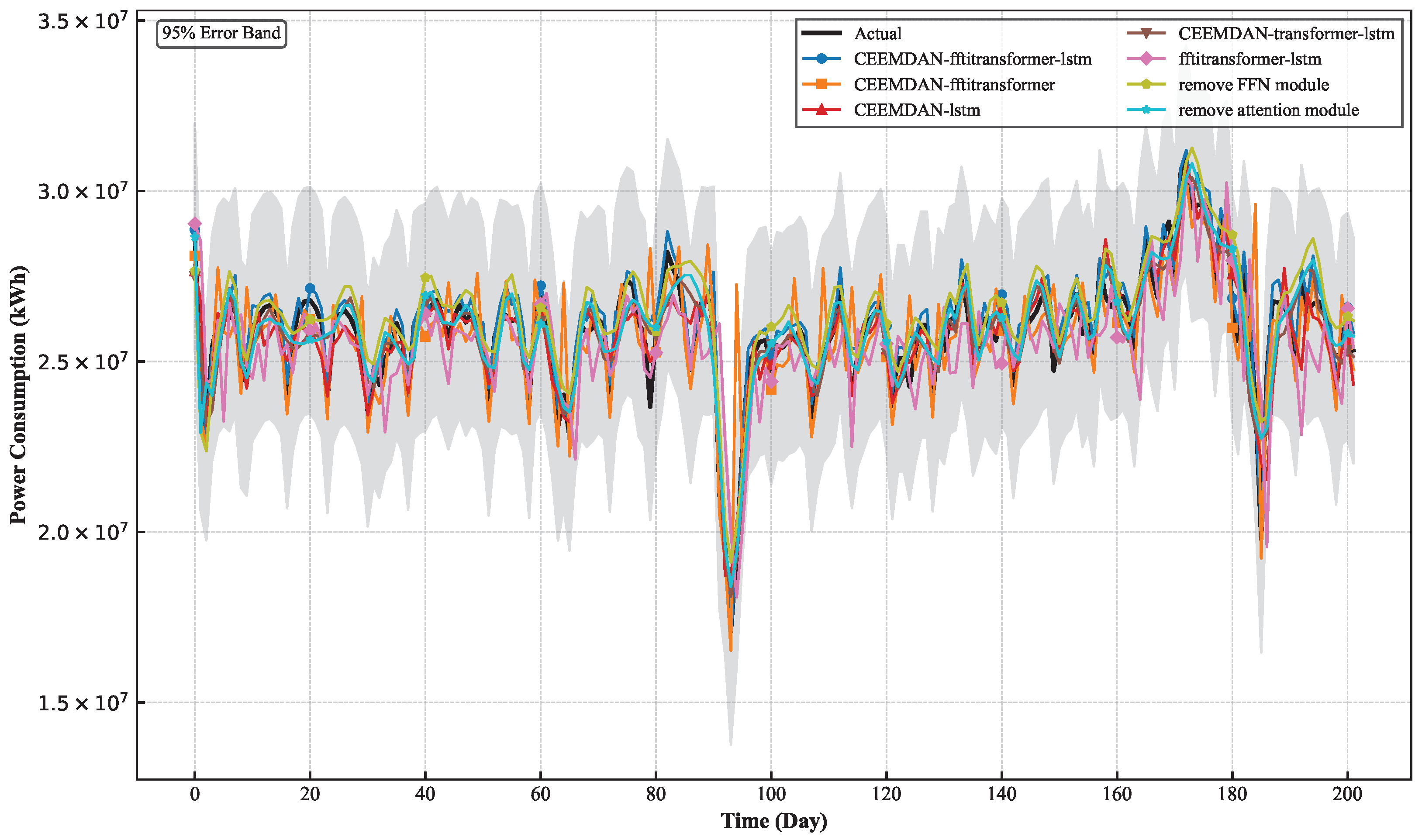
4.6.2. The Influence of Different Modules

To validate the superiority of our proposed model, we analyze the contributions of the following six modules to the prediction performance: CEEMDAN signal decomposition, FFT, iTransformer, iTransformer‘s attention module, iTransformer’s FFN module, and LSTM. The results are presented in Table 3 and Figure 9.
By analyzing the experimental results of removing the Attention module and FFN module separately, it can be observed that the model’s performance decreased significantly. On average, R 2 dropped by 31%, while MAE, RMSE, and MAPE increased substantially. This demonstrates that both modules are crucial components of the iTransformer. The Attention module enhances feature extraction by modeling global dependencies, while the FFN module optimizes long-term trend prediction through nonlinear mapping. In integrated models that incorporate CEEMDAN decomposition, such as CEEMDAN-LSTM and CEEMDAN-FFT-iTransformer, the model’s ability to handle long- and short-term dependencies in the time series is significantly improved. Specifically, R 2 improves by approximately 16% and 26%, respectively, while the MAE, RMSE, and MAPE values are remarkably reduced. Although these integrated models achieved an initial improvement in prediction accuracy, further enhancements are realized when the intrinsic mode functions (IMFs) obtained from the CEEMDAN decomposition are processed separately according to their distinct characteristics using different modules (iTransformer and LSTM).
Finally, by introducing an FFT module to extract the frequency domain features of the IMFs and passing them to the iTransformer module, we construct the complete CEEMDAN-FFT-iTransformer-LSTM model. This combined model achieves an R² value close to 1, and its error metrics are significantly lower compared with the other models. These results demonstrate that our model not only captures the complex dependencies within the signal effectively but also processes components across different frequencies efficiently, thereby exhibiting outstanding time series modeling and prediction capabilities.

5. Conclusions

In this paper, we proposed an integrated model, CEEMDAN-FFT-iTransformer-LSTM, for electricity time series forecasting. This model integrates multiple modules for deep feature extraction of power time series: CEEMDAN signal decomposition decouples the original power time series into multi-band intrinsic mode functions (IMFs) for frequency-specific processing; the FFT module converts time-domain signals into frequency-domain features and fuses them with temporal characteristics to construct a multidimensional input space; iTransformer tokenizes entire feature sequences through multi-head attention mechanisms to capture transient fluctuations in high-frequency components, while the LSTM network leverages gated mechanisms to extract long-term patterns from low-frequency IMFs. Moreover, We incorporated weather factors as supplementary features to assist prediction in our study. This complementary approach enables synergistic feature extraction across modules, achieving breakthrough performance in global temporal modeling for power forecasting.
Specifically, the model achieved R 2 = 0.905, MAE = 413,919, MAPE = 1.67% on the Hangzhou dataset, exhibiting significant performance advantages compared with other models. However, it should be noted that although our proposed framework has higher computational complexity compared to traditional models, resulting in relatively longer prediction time, the increase in time cost (38%) is significantly less than the improvement in model performance (50%).
The proposed CEEMDAN-FFT-iTransformer-LSTM model provides a powerful solution for ensuring stability, enhancing prediction accuracy, and optimizing scheduling in modern power systems.
  • Firstly, the model accurately captures both the short-term fluctuations and long-term trends of power loads, substantially improving forecasting accuracy. This not only aids power companies in optimizing the scheduling of generation and energy storage systems, thereby reducing unnecessary energy waste and operating costs, but also decreases the demand for large-scale storage systems.
  • Secondly, the stability of the power grid relies on balancing power supply and demand. The high-precision load forecasting provided by our model can significantly reduce power fluctuations, thereby mitigating safety issues associated with such fluctuations. A more stable power supply enhances grid safety and delivers more reliable power services to consumers.
  • Lastly, our model offers high-precision data support and optimized scheduling capabilities for smart grids, fostering the intelligent development of the power system.
However, it should be acknowledged that due to data confidentiality, this study is only based on power consumption data from Hangzhou. The applicability of the model to datasets from other regions with different characteristics has not been verified. This is a limitation of our research. In the future, we will conduct multi-regional benchmarking based on this, systematically considering multi-dimensional influencing factors, such as the power supply-demand relationship, grid topology, climate characteristics, and policy regulations. While improving the model’s cross-regional and cross-domain generalization capabilities, we will also enhance its adaptability and interpretability to complex scenarios in power systems.

Author Contributions

Conceptualization, Y.J. and W.S.; Data curation, Y.J.; Investigation, Y.J. and W.S.; Methodology, Y.J. and W.S.; Validation, Y.J. and W.S.; Writing—original draft, Y.J.; Writing—review and editing, W.S. and C.Q.W. All authors have read and agreed to the published version of the manuscript.

Funding

This research received no external funding.

Data Availability Statement

The data presented in this study are available on request from the corresponding author. The data are not publicly available due to privacy and confidentiality concerns.

Acknowledgments

The authors would like to thank the technical support provided by Dongliang Chu and Hao Tian.

Conflicts of Interest

The authors declare no conflicts of interest.

References

  1. Liu, D. International energy agency (IEA). In The Palgrave Encyclopedia of Global Security Studies; Springer: Berlin/Heidelberg, Germany, 2023; pp. 830–836. [Google Scholar]
  2. Maheswaran, D.; Rangaraj, V.; Kailas, K.J.; Kumar, W.A. Energy efficiency in electrical systems. In Proceedings of the 2012 IEEE International Conference on Power Electronics, Drives and Energy Systems (PEDES), Bengaluru, India, 16–19 December 2012; IEEE: New York, NY, USA, 2012; pp. 1–6. [Google Scholar]
  3. Van Heddeghem, W.; Lambert, S.; Lannoo, B.; Colle, D.; Pickavet, M.; Demeester, P. Trends in worldwide ICT electricity consumption from 2007 to 2012. Comput. Commun. 2014, 50, 64–76. [Google Scholar] [CrossRef]
  4. McRuer, D.T.; Graham, D.; Ashkenas, I. Aircraft Dynamics and Automatic Control; Princeton University Press: Princeton, NJ, USA, 2014; Volume 2731. [Google Scholar]
  5. Mourshed, M.; Robert, S.; Ranalli, A.; Messervey, T.; Reforgiato, D.; Contreau, R.; Becue, A.; Quinn, K.; Rezgui, Y.; Lennard, Z. Smart grid futures: Perspectives on the integration of energy and ICT services. Energy Procedia 2015, 75, 1132–1137. [Google Scholar] [CrossRef]
  6. Khalil, M.I.; Jhanjhi, N.; Humayun, M.; Sivanesan, S.; Masud, M.; Hossain, M.S. Hybrid smart grid with sustainable energy efficient resources for smart cities. Sustain. Energy Technol. Assessments 2021, 46, 101211. [Google Scholar] [CrossRef]
  7. Pao, H.T. Comparing linear and nonlinear forecasts for Taiwan’s electricity consumption. Energy 2006, 31, 2129–2141. [Google Scholar] [CrossRef]
  8. Zhang, B.; Yin, J.; Jiang, H.; Chen, S.; Ding, Y.; Xia, R.; Wei, D.; Luo, X. Multi-source data assessment and multi-factor analysis of urban carbon emissions: A case study of the Pearl River Basin, China. Urban Clim. 2023, 51, 101653. [Google Scholar] [CrossRef]
  9. Efekemo, E.; Saturday, E.; Ofodu, J. Electricity demand forecasting: A review. Educ. Res. IJMCER 2022, 4, 279–301. [Google Scholar]
  10. Lai, X.; He, M.; Hu, W.; Zhang, Y.; Du, P.; Liu, R.; Song, X.; Zheng, T. Multi-factor Electric Load Forecasting Based on Improved Variational Mode Decomposition and Deep Learning. Comput. Eng. 2025, 51, 375–386. [Google Scholar] [CrossRef]
  11. Li, S. FFT-CNN-LSTM-Based Short-Term Electric Load Forecasting. Master’s Thesis, Nanchang University, Nanchang, China, 2021. [Google Scholar]
  12. Hearst, M.; Dumais, S.; Osuna, E.; Platt, J.; Scholkopf, B. Support vector machines. IEEE Intell. Syst. Their Appl. 1998, 13, 18–28. [Google Scholar] [CrossRef]
  13. Breiman, L. Random forests. Mach. Learn. 2001, 45, 5–32. [Google Scholar] [CrossRef]
  14. Muzaffar, S.; Afshari, A. Short-term load forecasts using LSTM networks. Energy Procedia 2019, 158, 2922–2927. [Google Scholar] [CrossRef]
  15. Liu, Y.; Hu, T.; Zhang, H.; Wu, H.; Wang, S.; Ma, L.; Long, M. itransformer: Inverted transformers are effective for time series forecasting. arXiv 2023, arXiv:2310.06625. [Google Scholar]
  16. Morid, M.A.; Sheng, O.R.L.; Dunbar, J. Time series prediction using deep learning methods in healthcare. ACM Trans. Manag. Inf. Syst. 2023, 14, 1–29. [Google Scholar] [CrossRef]
  17. Zhu, S.; Ma, H.; Chen, L.; Wang, B.; Wang, H.; Li, X.; Gao, W. Short-term load forecasting of an integrated energy system based on STL-CPLE with multitask learning. Prot. Control Mod. Power Syst. 2024, 9, 71–92. [Google Scholar] [CrossRef]
  18. Li, B.; Zhang, J.; He, Y.; Wang, Y. Short-term load-forecasting method based on wavelet decomposition with second-order gray neural network model combined with ADF test. IEEE Access 2017, 5, 16324–16331. [Google Scholar] [CrossRef]
  19. Zhang, Y.; Li, C.; Jiang, Y.; Sun, L.; Zhao, R.; Yan, K.; Wang, W. Accurate prediction of water quality in urban drainage network with integrated EMD-LSTM model. J. Clean. Prod. 2022, 354, 131724. [Google Scholar] [CrossRef]
  20. Cao, J.; Li, Z.; Li, J. Financial time series forecasting model based on CEEMDAN and LSTM. Phys. A Stat. Mech. Its Appl. 2019, 519, 127–139. [Google Scholar] [CrossRef]
  21. Schwarz, K.; Sideris, M.; Forsberg, R. The use of FFT techniques in physical geodesy. Geophys. J. Int. 1990, 100, 485–514. [Google Scholar] [CrossRef]
  22. Jha, A.; Dorkar, O.; Biswas, A.; Emadi, A. iTransformer Network Based Approach for Accurate Remaining Useful Life Prediction in Lithium-Ion Batteries. In Proceedings of the 2024 IEEE Transportation Electrification Conference and Expo (ITEC), Rosemont, IL, USA, 19–21 June 2024; IEEE: New York, NY, USA, 2024; pp. 1–8. [Google Scholar]
  23. Voita, E.; Talbot, D.; Moiseev, F.; Sennrich, R.; Titov, I. Analyzing multi-head self-attention: Specialized heads do the heavy lifting, the rest can be pruned. arXiv 2019, arXiv:1905.09418. [Google Scholar]
  24. Bebis, G.; Georgiopoulos, M. Feed-forward neural networks. IEEE Potentials 1994, 13, 27–31. [Google Scholar] [CrossRef]
  25. Cavus, M.; Dissanayake, D.; Bell, M. Deep-Fuzzy Logic Control for Optimal Energy Management: A Predictive and Adaptive Framework for Grid-Connected Microgrids. Energies 2025, 18, 995. [Google Scholar] [CrossRef]
  26. Cavus, M.; Ugurluoglu, Y.F.; Ayan, H.; Allahham, A.; Adhikari, K.; Giaouris, D. Switched auto-regressive neural control (S-ANC) for Energy Management of Hybrid Microgrids. Appl. Sci. 2023, 13, 11744. [Google Scholar] [CrossRef]
  27. He, Y.L.; Chen, L.; Gao, Y.; Ma, J.H.; Xu, Y.; Zhu, Q.X. Novel double-layer bidirectional LSTM network with improved attention mechanism for predicting energy consumption. ISA Trans. 2022, 127, 350–360. [Google Scholar] [CrossRef] [PubMed]
  28. Kalpakis, K.; Gada, D.; Puttagunta, V. Distance measures for effective clustering of ARIMA time-series. In Proceedings of the 2001 IEEE International Conference on Data Mining, San Jose, CA, USA, 29 November–2 December 2001; IEEE: New York, NY, USA, 2001; pp. 273–280. [Google Scholar]
  29. Tokgöz, A.; Ünal, G. A RNN based time series approach for forecasting turkish electricity load. In Proceedings of the 2018 26th Signal Processing and Communications Applications Conference (SIU), Izmir, Turkey, 2–5 May 2018; IEEE: New York, NY, USA, 2018; pp. 1–4. [Google Scholar]
  30. Livieris, I.E.; Pintelas, E.; Pintelas, P. A CNN–LSTM model for gold price time-series forecasting. Neural Comput. Appl. 2020, 32, 17351–17360. [Google Scholar] [CrossRef]
  31. Zhang, K.; Gençay, R.; Yazgan, M.E. Application of wavelet decomposition in time-series forecasting. Econ. Lett. 2017, 158, 41–46. [Google Scholar] [CrossRef]
  32. Francia, G.A., III; El-Sheikh, E. NERC CIP standards: Review, compliance, and training. In Global Perspectives on Information Security Regulations: Compliance, Controls, and Assurance; IGI Global Scientific Publishing: Hershey, PA, USA, 2022; pp. 48–71. [Google Scholar]
Figure 1. Components and sensor deployment in the power system.
Electronics 14 02036 g001
Figure 2. Framework of the CEEMDAN-FFT-iTransformer-LSTM model.
Electronics 14 02036 g002
Figure 3. The daily electricity consumption data of Hangzhou.
Electronics 14 02036 g003
Figure 4. Temperature data for Hangzhou.
Electronics 14 02036 g004
Figure 5. Experiments on the hyperparameters {lookback_len, epochs, and learning rate} and comparison of errors with different hyperparameters. (a) lookback_len; (b) epochs; and (c) learning rate.
Electronics 14 02036 g005
Figure 6. Signal decomposition values of CEEMDAN.
Electronics 14 02036 g006
Figure 7. Correlation graph between temperature and various IMF components.
Electronics 14 02036 g007
Figure 8. Predicted values of different models.
Electronics 14 02036 g008
Figure 9. Predicted values of removing different modules.
Electronics 14 02036 g009
Table 1. Hyperparameter configuration and justifications.
ComponentHyperparameterValue
iTransformerNumber of Attention Heads4
Model Dimension ( d model )128
Feed-Forward Dimension ( d ff )512
Lookback_len13
LSTMHidden Units128
Number of Layers2
Lookback_len13
Training ProtocolBatch Size64
OptimizerAdam
Learning Rate0.0005
Dropout Rate0.1
Epochs30
Table 2. Performance comparison of different models on the electricity dataset.
Model R 2 MAERMSEMAPERuning Time
ARIMA0.4082978,3641,373,6653.9482437.79 s
RNN0.4216947,7891,318,7333.7781350.45 s
CNN-LSTM0.4561839,5691,222,9343.4421508.21 s
Wavelet-FFTiTransformer-lstm0.6481752,2421,055,7562.8513730.46 s
CEEMDAN-FFTiTransformer-lstm0.9055413,919557,1461.6794691.21 s
Table 3. Performance comparison of removing different modules on our electricity dataset.
Model R 2 MAERMSEMAPE
FFTiTansformer-lstm0.4105933,4431,352,4833.7655
CEEMDAN-FFTiTansformer0.5735808,9201,106,9763.0205
Remove attention module0.6141784,584942,8122.934
Remove FFN module0.6237764,367931,7232.914
CEEMDAN-lstm0.6756735,593919,8462.8432
CEEMDAN-iTransformer-lstm0.7878654,113831,3252.2797
CEEMDAN-FFTiTransformer-lstm0.9055413,919557,1461.6794
Disclaimer/Publisher’s Note: The statements, opinions and data contained in all publications are solely those of the individual author(s) and contributor(s) and not of MDPI and/or the editor(s). MDPI and/or the editor(s) disclaim responsibility for any injury to people or property resulting from any ideas, methods, instructions or products referred to in the content.

