Blockage Prediction of an Urban Wireless Channel Characterization Using Classification Artificial Intelligence

Abstract

The global deployment of 5G wireless networks has introduced significant advancements in data rates, latency, and energy efficiency. However, the rising demand for immersive applications (e.g., virtual and augmented reality) necessitates even higher data rates and lower latency, driving research toward sixth-generation (6G) wireless networks. This study addresses a major challenge in post-5G communication: mitigating signal blockage in high-frequency millimeter-wave (mmWave) bands. This paper proposes a novel framework for blockage prediction using AI-based classification techniques to enhance signal reliability and optimize connectivity. The proposed framework is evaluated comprehensively using performance metrics such as accuracy, precision, recall, and F1-score. Notably, the NN Model 4 achieves a classification accuracy of 99.8%. Comprehensive visualizations—such as learning curves, confusion matrices, ROC curves, and precision-recall plots—highlight the model’s performance. This study contributes to the development of AI-driven techniques that enhance reliability and efficiency in future wireless communication systems.

1. Introduction

The development of sixth-generation (6G) wireless networks is driven by the growing demand for ultra-high data rates, ultra-low latency, and massive connectivity. These capabilities are essential to enable emerging technologies, such as immersive virtual reality (VR), autonomous systems, and large-scale Internet of Things (IoT) deployments, thus necessitating the next evolutionary leap to 6G [1]. A key enabler of 6G is the use of millimeter-wave (mmWave) frequencies (30–300 GHz), which provide vast spectrum resources to support ultra-fast data transmission and enhanced bandwidth capabilities [2]. However, mmWave bands present significant challenges in wireless communication, primarily due to their unique propagation characteristics.

This paper addresses a fundamental challenge in mmWave systems: predicting signal blockage and managing signal degradation in complex urban environments. The proposed approach leverages AI-based classification models to predict signal blockage events in real-time. The classification strategy differentiates between blockage and non-blockage conditions based on path loss thresholds derived from empirical data and mmWave propagation models. By applying machine learning (ML) methods such as logistic regression, support vector machine (SVM), and neural networks (NNs), this study advances the development of intelligent, adaptive communication systems that maintain robust connectivity in dynamic environments.

This study leverages multiple classification techniques, such as logistic regression, SVM, and NNs, to optimize signal detection and minimize blockage in high-frequency 6G systems. This approach classifies signals based on path loss. Specifically, it uses corrupted path loss strength values to predict blockage. Our mechanism is based on the corrupted path loss strength value. Thus, $PL$ ≥ 120 ⇒ class zero indicates a signal blockage occurrence, while $PL$ < 120 ⇒ class one states that the signal is not blocked, as shown in Figure 1. An assumption of 120 dB as a maximum path loss value allows the receiver to detect and decode the transmitted signal; otherwise, the signal is considered noise [3]. Similarly, reference [4] used machine learning techniques to model the loss of the mmWave path and demonstrated that the strength of the received signal below a critical threshold (such as 120 dB) indicates a high probability of blockage. Moreover, the threshold of 120 dB aligns with the receiver sensitivity limits of modern mmWave systems. According to system link budget calculations, beyond this value, the signal-to-noise ratio (SNR) often drops below the minimum required for decoding, effectively making the signal indistinguishable from noise. This is consistent with established propagation models, such as the NYUSIM channel model for 5G mmWave, which reports that urban microcell environments exhibit path loss values in the range of 100–140 dB, with 120 dB often marking the transition from weak but detectable signals to complete signal degradation [5]. In current 5G systems, blockage prediction models often define signal blockage around similar path loss values. For example, the 3GPP TR 38.901 standard for mmWave propagation considers the path loss in urban scenarios and notes that beyond 120 to 130 dB, Non-Line-of-Sight (NLOS) conditions dominate, significantly reducing link reliability [6]. Furthermore, reference [7] analyzed mmWave propagation at 140 GHz and demonstrated that path loss values exceeding 120 dB indicate significant blockage effects. Performance is then evaluated using metrics such as accuracy, precision, recall, and F1-score.

By leveraging the results of these AI classification techniques, 6G cellular systems can intelligently adapt to the dynamic nature of mmWave channels. This paves the way for:

• Robust communication: Proactive mitigation of signal degradation, blockage, and channel impairments.
• Enhanced user experience: Consistent high-speed data delivery and reduced latency for users.
• Improved network efficiency: Optimal resource allocation, minimizing wasted bandwidth, and maximizing network capacity.

To summarize the contribution of the paper that involves signal enhancement, blockage avoidance, and AI-driven signal optimization in high mmWave communication, the following points are highlighted:

• Signal Blockage Mitigation: We propose a novel mechanism to enhance signal reception by addressing the inherent susceptibility of mmWave communication to blockage caused by obstacles, ensuring reliable connectivity in dynamic environments.
• AI-Driven Signal Optimization: Leverages artificial intelligence on the reception side by intelligently selecting the optimal signal path or beam, dynamically adapting to changing conditions, and maximizing communication efficiency.
• Enhanced High-Frequency Utilization: Demonstrates methods to optimize high-mmWave frequency bands, overcoming propagation challenges to unlock their potential for reliable communications.

Finally, this work involves a discussion of the challenges and future research directions in the integration of AI in 6G wireless communication technology. The results of this study provide information on the potential benefits of AI in future 6G wireless communications and highlight the need for further research in this area.

The structure of this manuscript is as follows: Section 1 introduces 6G wireless systems, followed by a general background in Section 2. Section 3 presents 6G use cases, while Section 4 discusses the network architecture. Section 5 outlines key challenges. Section 6 examines the integration of AI and Section 7 presents results related to block prediction. Section 8 and Section 9 provide future directions and the conclusion, respectively.

2. Background

Wireless channel modeling has traditionally relied on deterministic and empirical methods. Examples include ray-tracing techniques and statistical propagation models, which have been fundamental in characterizing signal behavior across diverse environments. However, with the adoption of mmWave and terahertz (THz) bands in 6G, AI and ML have emerged as powerful alternatives to traditional modeling approaches [8,9].

Ray-tracing models simulate radio wave propagation deterministically by accounting for reflections, diffraction, and scattering from obstacles such as buildings and vehicles. These models offer high accuracy when detailed environmental information is available. Similarly, empirical models, such as those proposed by Seidel and Rappaport [3], use statistical data from measurements to estimate path loss. Although computationally efficient and simple, empirical models often fail to generalize well to dynamic environments.

To address the challenges in mmWave propagation, AI-based models have been extensively explored. Unlike traditional methods, AI models learn complex patterns directly from data, enabling them to predict channel behaviors, such as path loss, blockage, and link reliability, without relying on detailed environmental parameters. Ghassemi et al. [10] proposed a Transformer-based (ViT) approach for vision-aided blockage prediction, which dynamically switches between the mmWave and sub-6 GHz bands to enhance throughput and ensure reliable connectivity. Similarly, Charan et al. [11] developed a deep learning model that integrates visual and wireless channel data to proactively predict signal blockages.

The evolution from 5G to 6G represents not just an increase in data rates but also a paradigm shift in network intelligence, spectrum utilization, and service delivery. The 6G network is envisioned to operate in high-frequency bands such as millimeter wave (30 to 300 GHz) and terahertz (0.1 to 10 THz), unlocking vast spectral resources and enabling extreme data rates of up to several terabits per second [2,12]. However, these bands present severe propagation challenges, including increased free-space path loss, susceptibility to atmospheric absorption, and vulnerability to physical blockages [13].

The attenuation in mmWave and THz bands is highly frequency-dependent. As frequency increases, signals experience greater absorption by atmospheric gases—particularly oxygen and water vapor—as well as materials, thus limiting the transmission range and the overall reliability of the link [14]. Building, vegetation, vehicle, and even human body obstructions can rapidly attenuate signal strength, resulting in service interruptions [15]. As a result, predictive and adaptive mechanisms are critical for sustaining link quality in 6G environments.

To mitigate these challenges, recent research has focused on integrating artificial intelligence (AI) and machine learning (ML) techniques to predict blockage events and dynamically manage wireless resources [16]. AI models have demonstrated high efficacy in analyzing complex propagation environments by learning from large datasets generated through ray tracing, real-world measurements, or simulations like NYUSIM [5,17]. Prominent among these are classification algorithms such as support vector machine (SVM), logistic regression (LR), and neural networks (NNs), which effectively differentiate blocked from non-blocked scenarios using features like path loss, delay spread, angles of arrival/departure, and received power.

Furthermore, 3GPP TR 38.901 and other standardization efforts confirm that mmWave signals typically become undetectable when the path loss exceeds 120–130 dB in urban environments [6]. This threshold has been widely adopted in blockage classification research and is used to define binary classes in many machine learning frameworks. The ability of AI models to preemptively identify when a blockage is likely allows networks to switch to alternative beams or fallback paths, thereby ensuring consistent quality of service.

Thus, this work contributes to the growing body of research that leverages AI classification models to predict signal blockages in high-frequency wireless channels, offering an intelligent solution to one of the key challenges in 6G network deployment.

Millimeter-wave (mmWave) communication differs from sub-6 GHz systems due to its distinct signal behavior. Several key characteristics define its propagation:

High Path Loss: Due to their much shorter wavelengths, mmWave signals experience significantly higher free-space path loss, especially as frequency increases. In dense urban microcell environments, this loss can range from 100 dB to 140 dB, often exceeding the 120 dB mark, at which point, maintaining a reliable connection becomes a real challenge [7].

Dynamic Blockage: One of the major hurdles in mmWave systems is their sensitivity to physical obstructions. Everyday urban features like buildings, trees, and even people can interrupt the signal. Studies [18] show that dynamic situations such as passing vehicles or pedestrians can cause sudden and severe drops in signal quality, leading to unstable connections.

NLOS Conditions: In cities, direct Line-of-Sight (LOS) between transmitter and receiver is often blocked. In these cases, the system relies on reflected or diffracted signals, which typically have weaker power, longer delays, and more variability. Tools such as NYUSIM and ray-tracing models [7] demonstrate how much performance can suffer under NLOS conditions, making smart mitigation strategies essential. Author: Done Environmental Sensitivity: mmWave signals are also highly affected by their surroundings. Factors like the materials of nearby surfaces, their texture, and even weather conditions can influence how signals propagate. Atmospheric absorption and scattering make real-time modeling and prediction even more complex.

Because of these challenges, there is a growing need for advanced, adaptive technologies—particularly AI-driven approaches—for predicting blockages and adjusting links on the fly. These innovations will be key to making mmWave viable in future 6G networks.

3. 6G Radio

The 6G wireless network is empowering different new applications with the application of several innovations [19]. Integrating the 5G New Radio (NR) framework with evolving wireless network architectures presents a key challenge for future generations [20,21]. Although 5G NR operates in the mmWave band, beamforming is essential for enhancing signal gain. It plays a critical role in improving link reliability and coverage within the mmWave spectrum. The 6G network is anticipated to outperform existing networks by supporting advanced applications and services with unprecedented performance requirements. These networks are expected to meet the growing demand for ultra-high data rates, ultra-low latency, wide coverage, high reliability, and consistent service quality.

Channel modeling has always been a critical component of wireless communication systems across all generations. Wireless channels are unpredictable due to many reasons such as movement that affects the propagation of the signal and blockage. Traditionally, wireless channel estimation relied on deterministic or empirical methods. In 5G+ and future networks, AI and ML techniques are increasingly employed to enhance the accuracy of path loss estimation. Calculating the received signal strength is also useful for determining base station coverage [22].

These models use ray optical laws to calculate the reflected rays and diffraction of electromagnetic waves during scene or location reproduction. Ray tracing, an optical modeling approach, considers all potential paths a signal may traverse between the transmitter and receiver. It then adds up the power from each of these paths to determine the total received power at a specific location. Ray tracing algorithms account for multiple reflections and obstructions by simulating visibility and reflection conditions along the signal path. Such models have been widely implemented in commercial and academic wireless simulation tools. Accurate modeling of multipath reflections is essential in ray tracing, especially in environments with dense obstructions. The ray tracing calculation determines all pertinent beams for each collection point of varied focuses [7].

To date there have not been commercial 6G applications but researchers are working on these, and the following subsections may contribute to this.

3.1. Extensive Machine-to-Machine Interaction

Machine-type communication handles communication between machines without the need for human intervention. The number of connected devices is estimated to reach billions of devices. Extensive machine-to-machine interaction is described as one of the essential use cases of 5G NR for communication among these massive amounts of connected devices. Extensive machine-to-machine interaction can be used for various purposes, including wellness monitoring, the board of armada and scheduled operations, autonomous driving, industrial facility mechanization, intelligent metering, surveillance, and security [23].

3.2. Network Design for Network Transition Past 5G/6G

D2D, OFDMA NOMA, SCA, MIMO, and massive MIMO are essential improvements in the 5G organization architecture. These developments have concentrated on meeting all of the 5G requirements that are recognized as the 2020 prerequisites. The System Coordinated Access (SCA) network constructs the inclusion and offloads the data flow. MIMO helps broaden the diversity achieved to accommodate the most significant number of clients. Massive MIMO is an expansion of conventional MIMO frameworks that aids in enabling massive availability in the business. Mental Radio is another essential innovation for utilizing the accessible groups in the range by changing various bounds for concurrent correspondence. According to 3GPP release 15, the leading standard air interface for the 5G organization is 5G New Radio. In 5G NR, 3GPP has established two frequency groups. These two frequency bands are less than 6 GHz (FR1) and greater than 24 GHz (FR2). The FR2 spectrum incorporates the millimeter-wave band, which uses high frequencies to improve information speeds. The diverse range and numerology provide full inclusion and better information rates. Because high frequencies are often associated with significant proliferation problems, mmWave execution is constrained to narrow locations. The mmWave restriction can be removed by increasing the radio wire gain by beamforming. Beamforming is a technique for directing the most extreme force of a sign toward the client’s direction. An investigation of the association of wireless frequency with the path loss for a range of frequencies from 0.1 GHz to 100 GHz can be seen in Figure 2. The power of the frequencies is shown in the figure; frequencies such as 2, 18, 40, 54, 68, and 82 GHz exhibit varying degrees of path loss. In general, higher frequencies correspond to greater path loss and vice versa.

While early 5G networks operated primarily in sub-6 GHz bands, the demand for higher data throughput led to the adoption of mmWave frequencies. The 6G network is expected to utilize terahertz (THz) frequencies to support data rates reaching up to terabits per second [25]. Optical Wireless Communication (OWC) is emerging as a promising solution, with visible light frequencies offering substantial potential for data transmission. Visible Light Communication (VLC) refers to data transmission using visible light wavelengths, offering high-speed and interference-free communication [26]. Notably, visible light wavelengths enable high data rates (in the terabit-per-second range) and support energy-efficient, environmentally friendly communication. Future forms will focus on reduced power consumption and increased battery life by delivering energy-efficient methods.

4. 6G Challenges and Opportunities

This section outlines the key challenges and potential opportunities associated with sixth-generation (6G) wireless communication systems.

4.1. Material Internet Challenges

Integrating communication, management, and computing systems into a unified framework is one of the primary technical challenges in realizing the vision of the tactile internet. The flexible communication framework is integrated into a wireless network. It combines hardware and virtual network components to support dynamic control systems. The tactile internet is still in its early developmental stages. Several unresolved evaluation challenges still need to be addressed. In addition to physical layer challenges—such as waveform design and robust scheduling—with intelligent control-plane and user-plane reducing end-to-end delay, it is critical to focus on flexible network coding techniques, and adaptive routing algorithms. Similarly, security is likely the most basic requirement for material internet applications. To protect against malicious attacks, robust security and trust assurance mechanisms must be implemented. The fundamental design principle of wireless tactile systems should be to empower users through assisted decision-making, rather than fully replacing human roles or control [27].

4.2. Non-Technical Challenges

The evolution of 6G must address not only technical challenges but also a variety of non-technical issues, including industry resistance, spectrum allocation policies, regulatory frameworks, and legal considerations. Unlike 5G, 6G is expected to be deeply integrated into all aspects of human life and industrial activity, fostering stronger collaboration across various sectors. Versatile correspondence will entail not being restricted to its specific field but collaborating intimately with different ventures/fields. In any case, the natural approach or benefits of certain customary methods would directly or, by implication, create industry obstructions to 6G. Another non-specific component is the range task and use rules. For instance, the 6G terahertz repeat will require composing assignments from various states and areas worldwide. A bound-together recurrence range should be spread as much as possible. Coordination with clients in other regions of the range, such as climate radar, should also be considered. In terms of plans and rules, satellite communications will face increasing constraints. A satellite’s correspondence circle and reach resources should be determined through individual interviews. Second, satellite correspondences will have more issues when trading through overall meandering than through traditional natural interchanges [25]. As of now, a few powerful nations and a few industry interests are effectively building satellite communication frameworks. Organizing connections between these satellite communication frameworks which are conveyed freely to one another will be a complicated issue.

4.3. Application Segmentation

Application segmentation is analogous to the client-side in network slicing. It aids in applications such as haptic communication, remote surgery, autonomous vehicles, and many more. Several utilization cuts have built-in application cutting layers in light of the different uses. The layer then gathers all the insights regarding the requested application and encodes them as execution measurements. These measurements will incorporate the required quality of service, inertness necessities, and the required transfer speed. At the RAN segmentation layer, a cut is chosen from the generally present cuts and put away in the store because of the exhibition measurements. If, regardless, the required RAN cut is absent, a new cut is created by the NFL. Segmentation engineering creates different new services [28,29].

5. Knowledge of Artificial Intelligence

Recent advancements in artificial intelligence (AI) have significantly expanded its applications across both academic research and commercial sectors. AI has rapidly found use in cognitive radios, remote sensing, computer vision, and network management within communication and signal processing domains [30]. In wireless communications, AI algorithms have demonstrated value in emerging technologies, such as massive MIMO, which require efficient channel estimation and optimization. Such tasks typically do not yield low-complexity optimal solutions in complex wireless environments; therefore, the parallel processing capabilities inherent in AI can be leveraged to improve computational efficiency. Modern wireless communication networks adopt a layered architecture, where each layer is responsible for specific functions, including those that support AI integration. Advanced AI algorithms are increasingly bridging the gap between protocol layers, enabling more holistic optimization across the wireless network stack [16]. In any case, this part is coordinated considering the current layers to provide a noticeable way to explore numerous unpreventable computer-based intelligence applications. It is critical to note that simulated intelligence is a good idea that incorporates several branches that cut across different areas, for example, mechanical innovation, normal language handling, AI, and PC vision.

5.1. Artificial Intelligence in the Physical Layer

Traditionally, physical layer modeling has been model-based, where mathematical structures are defined and refined within specific constraints to meet predetermined performance requirements. For example, a channel model is typically designed to work alongside parametric methods to guide channel estimation. Researchers have recently adopted AI techniques to model wireless communication channels and estimate channel state information (CSI) parameters [31,32].

5.2. Artificial Intelligence in Wireless Networks

The availability of rich datasets across various layers of wireless systems makes them well suited for the application of AI-based solutions. Researchers have successfully applied reinforcement learning strategies to routing protocol design in wireless sensor networks, achieving more energy-efficient control mechanisms for distributed sensor environments. In vehicular communication systems, predictive models based on real-time data have shown superior accuracy compared to traditional probabilistic models, especially given the dynamic nature of vehicle movement [33]. Beyond advancements in computational techniques, one major challenge lies in data storage and management, particularly within centralized cloud-based data centers. Such centralized processing can cause significant delays in executing time-sensitive tasks, especially for devices distributed over large geographic areas. Moreover, centralized computing is not ideal for maintaining data privacy and addressing processing constraints in distributed systems. Edge AI enables localized devices to perform computation and decision-making tasks, thereby alleviating the limitations of centralized cloud systems [34]. However, edge devices may face potential overload, as they typically lack the processing power of a centralized cloud infrastructure. Ongoing research efforts have focused on the following strategies to address these challenges:

• Improving the processing capabilities of edge hardware.
• Enhancing coordination between edge and central processing units to optimize task allocation.

5.3. Artificial Intelligence in Network Administration and AI

Simulated intelligence is essential in the administration of organizations. With the rise in Software-Defined Networking (SDN) and Network Function Virtualization (NFV), large-scale data collection has become significantly more accessible. This progress has enabled robust AI-based management and coordination mechanisms within 6G, paving the way for full network automation [16]. Specifically, the core domain of network administration presents several challenges, which can be broadly categorized as follows:

• Supervised learning: Commonly applied for traffic prediction, classification, and resource forecasting.
• Reinforcement learning: Effective in dynamic resource management and adaptive control.
• Unsupervised learning: Although less common, it offers promising use cases in anomaly detection and traffic pattern discovery.

6. Pervasive Artificial Intelligence Issues

During the early phases of 5G standardization, researchers explored the potential of artificial intelligence to enhance performance and operational efficiency. Specifically, AI algorithms can support tasks that are traditionally inefficient when performed manually, such as anomaly detection, resource allocation, and automated network management. However, these AI-driven solutions have yet to be fully adopted in global 5G deployments. While artificial intelligence (AI) is expected to drive a paradigm shift toward data-driven approaches in wireless communication, several unresolved challenges remain. There is still no consensus on the most effective algorithms for addressing unified challenges in small-scale networks, such as modulation and coding design, channel estimation, and resource allocation [30]. Practically distributed work promises high precision or low complexity with either logical hypotheses or valuable informational collections. Furthermore, we note the lack of a powerful strategy for fair examination across all recommended arrangements due to differences in selected informational collections, assumptions, and assessment standards. A cautious collection cycle should be followed for organizations to recognize computations without losing general relevance. Second, the limited accessibility of value datasets hinders the testing and acceptance of suggested categorization or relapse estimates [35,36].

7. Results

The dataset used in this study was generated using the NYUSIM millimeter-wave channel simulator [17], configured for an urban microcell environment at a frequency of 145 GHz. In the simulation setup, both LOS (Line-of-Sight) and NLOS (Non-Line-of-Sight) conditions were mixed to accurately reflect urban microcell environments. The NYUSIM channel simulator inherently accounts for various urban obstacles, including buildings, vehicles, and other typical obstructions. The simulations were not limited to open spaces but incorporated realistic urban blockage scenarios to evaluate the performance of the classification models under diverse conditions. The generated Channel State Information (CSI) includes critical parameters such as the T-R separation distance (m), time delay (ns), received power (dBm), phase (rad), azimuth AoD, elevation AoD, azimuth AoA, elevation AoA, path loss (dB), and RMS delay spread (ns). To enable binary classification, a path loss threshold of 120 dB was employed to assign data to two classes. Prior to model training, the dataset underwent preprocessing, which included normalization of numerical features to ensure uniform scaling and enhance model convergence. Subsequently, the dataset was split into training and testing sets using a standard 80:20 ratio. This enabled effective training of the classification models—including logistic regression, support vector machine (SVM), and several neural network configurations—while ensuring reliable evaluation, using metrics such as accuracy, precision, recall, and F1-score on unseen data. Figure 3 illustrates the distribution of the path loss (dB) against the average T-R separation distance, highlighting the expected signal attenuation with increased distance.

This section analyzes the performance of classification models to uncover patterns in the dataset and evaluate their effectiveness in binary classification. Using performance metrics and visualizations, the study seeks to provide insights that support reliable decision-making in binary classification tasks.

For classification, we employ logistic regression, SVM, and an NN. Performance is evaluated using metrics like accuracy, precision, recall, and F1-score. Visualizations, such as learning curves, confusion matrices, ROC curves, and precision-recall curves, aid in assessing the models’ effectiveness.

The use of metrics and visualizations enables a thorough evaluation of model performance and enhances our understanding of binary variable analysis. Neural networks (NNs), logistic regression, and support vector machine (SVM) are AI classification techniques that have been implemented to predict the blockage occurrence during signal propagation.

In this section, classification models, such as an NN, logistic regression, and SVM, have been applied. The quality of these models is evaluated using metrics to assess model performance.

• Accuracy: Represents the proportion of correctly classified instances (blocked vs. non-blocked signals). While useful as an overall measure, it can be misleading for imbalanced datasets.
• Precision: Indicates the ability to avoid false positives, which is especially important in identifying blocked signals accurately.
• Recall: Measures the model’s ability to detect blocked signals, minimizing false negatives.
• F1-score: A harmonic mean of precision and recall, used to balance these metrics when they conflict.
• ROC Curve and AUC (Area Under the Curve): Demonstrate the model’s discriminative power across different classification thresholds, with higher AUC values indicating better performance.

Learning curve: The learning curve illustrates the relationship between the model’s accuracy and the size of the training dataset. It helps assess if the model would benefit from additional training data or if it has reached its maximum potential.

Accuracy: This represents the overall ability of the model to make correct predictions. A high accuracy result indicates that the model has a high rate of overall correct predictions.

$$\mathrm{Accuracy}={\displaystyle \frac{TP+TN}{TP+TN+FP+FN}}$$

(1)

where TP represents true positives, and TN stands for true negatives, while FP represents false positives and FN represents false negatives.

Precision: The model can avoid misclassifying negative instances as positive. High-precision results show that the model has a low rate of false positives.

$$\mathrm{Precision}={\displaystyle \frac{TruePositives}{TruePositives+FalsePositives}}$$

(2)

Recall: Represents the model’s ability to correctly identify positive instances. A high recall value indicates that the model has a low rate of false negatives and can identify most of the positive instances.

$$\mathrm{Recall}={\displaystyle \frac{TruePositives}{TruePositives+FalseNegatives}}$$

(3)

F1-Score: It is a general measure of the model’s precision, considering both the ability to avoid false positives and false negatives. A high F1-score means the test does well at avoiding both mistakes, striking a good balance between accuracy for positive things and accuracy for negative things.

$$\mathrm{F}1-\mathrm{Score}={\displaystyle \frac{2*Precision*Recall}{Precision+Recall}}$$

(4)

ROC Curve: The Receiver Operating Characteristic (ROC) curve shows how well a binary classification model performs at different levels of strictness. It does this by plotting how often it correctly identifies positive cases (recall) against how often it mistakenly identifies negative cases as positive across different thresholds [37].

Precision-Recall Curve: The precision-recall curve visualizes the trade-off between precision and recall at different classification thresholds. It plots precision on the y-axis and recall on the x-axis.

Initially, functions are created to efficiently apply the models and display the metrics. Then, a brief description of each model’s functioning is provided. Finally, the results of the regression models are discussed and analyzed.

7.1. Neural Networks (NNs)

Neural networks are a part of artificial intelligence that acts like a computer version of a brain [38]. Made up of simple processing units connected in layers, they mimic the way brains learn by passing information back and forth, usually called forward and backward propagation, as shown in Figure 4, and the output can be calculated using Equations (5) and (6).

$${\mathcal{L}}_{ϵ}(y,f(x,w))={\displaystyle \frac{1}{2}}\sum _{i=0}^k{(y_{k_i}-\widehat{y_{k_i}})}^2$$

(5)

where $\mathcal{L}$ represents the loss, y is the actual dependent value, and $\widehat{y_k}$ is the predicted value.

The predicted value of the neural network can be represented as follows. The equation for a neural network can be expressed in terms of its forward pass. A common form for a single-layer and multi-layer neural network is:

$$\widehat{y}=f\left(W·x+b\right)$$

(6)

$$\widehat{y_k}=\sum _{i=0}^k(w_{jk}·S\sum _{i=0}^k(w_{ij}{x}_i+b_j)+b_k)$$

(7)

Further details of forward and backward propagation are presented below.

7.1.1. Forward Pass

During the forward pass, the input data are propagated through the layers of the neural network to calculate the output. For a given layer l, the output $z^{\left(l\right)}$ is computed as:

$$z^{\left(l\right)}=W^{\left(l\right)}·a^{(l-1)}+b^{\left(l\right)},$$

(8)

where:

• $W^{\left(l\right)}$ is the weight matrix of layer l,
• $a^{(l-1)}$ is the activation from the previous layer,
• $b^{\left(l\right)}$ is the bias vector of layer l.

The activation $a^{\left(l\right)}$ of the current layer is then calculated using an activation function $f(·)$. For the ReLU (Rectified Linear Unit) activation function, this is expressed as:

$$a^{\left(l\right)}=max(0,z^{\left(l\right)}).$$

(9)

The final layer uses a sigmoid activation function for binary classification, defined as:

$$a^{\left(L\right)}={\displaystyle \frac{1}{1+e^{-z^{\left(L\right)}}}},$$

(10)

where L is the output layer.

7.1.2. Backpropagation

The backpropagation algorithm calculates the gradients of the loss function concerning the model parameters (W and b) to update them during training. This process involves the following steps.

7.1.3. Gradient of the Loss Function

The loss function L for binary classification is defined as:

$$L=-{\displaystyle \frac{1}{N}}\sum _{i=1}^N\left[y_i·log\left(p_i\right)+(1-y_i)·log(1-p_i)\right],$$

(11)

where:

• N is the number of samples,
• $y_i$ is the true label of the i-th sample,
• $p_i$ is the predicted probability for the i-th sample.

7.1.4. Weight and Bias Updates

For each layer l, the gradients of the loss function to the weights $W^{\left(l\right)}$ and biases $b^{\left(l\right)}$ are calculated as follows:

$${\displaystyle \frac{\partial L}{\partial W^{\left(l\right)}}}={\delta }^{\left(l\right)}·a^{{(l-1)}^T},$$

(12)

$${\displaystyle \frac{\partial L}{\partial b^{\left(l\right)}}}={\delta }^{\left(l\right)},$$

(13)

where ${\delta }^{\left(l\right)}$ is the error term for layer l, calculated as:

$${\delta }^{\left(l\right)}={\displaystyle \frac{\partial L}{\partial z^{\left(l\right)}}}·f^{\prime }\left(z^{\left(l\right)}\right).$$

(14)

Here, $f^{\prime }\left(z^{\left(l\right)}\right)$ is the derivative of the activation function $f(·)$. For the output layer, the error term is computed as:

$${\delta }^{\left(L\right)}=a^{\left(L\right)}-y,$$

(15)

where $a^{\left(L\right)}$ is the output activation, and y is the true label.

7.1.5. Propagation to Previous Layers

The error term for a hidden layer l is propagated backward as:

$${\delta }^{\left(l\right)}=\left(W^{{(l+1)}^T}·{\delta }^{(l+1)}\right)·f^{\prime }\left(z^{\left(l\right)}\right).$$

(16)

7.1.6. Parameter Update

Finally, the weights and biases are updated using the gradient descent algorithm:

$$W^{\left(l\right)}=W^{\left(l\right)}-\eta ·{\displaystyle \frac{\partial L}{\partial W^{\left(l\right)}}},$$

(17)

$$b^{\left(l\right)}=b^{\left(l\right)}-\eta ·{\displaystyle \frac{\partial L}{\partial b^{\left(l\right)}}},$$

(18)

where $\eta$ is the learning rate.

The forward and backpropagation processes enable the neural network to learn by iteratively updating its weights and biases to minimize the loss function. This mechanism allows the network to effectively predict signal blockages in high-frequency mmWave communication systems.

7.2. Support Vector Machine

Support vector machine (SVM) is a classification tool used in machine learning. SVM works by identifying a hyperplane in high-dimensional space that optimally separates the data points belonging to different classes. This hyperplane is defined by an equation of the form:

$$w^{T}x+b=0$$

(19)

where w is a weight vector representing the direction of the hyperplane and x is a data point, while b is the bias term that determines the position of the hyperplane and T denotes the transpose operation.

The main concept of SVM is to create a wide gap between the decision line (hyperplane) and the most important data points (support vectors) for each class. This gap is critical for the model’s ability to handle new, unseen data (generalization performance). By prioritizing a large margin, SVM seeks to build a strong decision boundary that can effectively separate the classes.

7.3. Logistic Regression

Logistic regression is an algorithm used for binary classification problems. This model predicts the chance of something belonging to a specific group by using a logistic function [39]. The logistic function is defined as:

$$f\left(x\right)={\displaystyle \frac{1}{1+e^{-z}}}$$

(20)

where z is a linear combination of the predictor variables:

$$z={\beta }_0+{\beta }_1{x}_1+{\beta }_2{x}_2+\dots +{\beta }_n{x}_n$$

(21)

Here, ${\beta }_0$, ${\beta }_1$, …, ${\beta }_n$ are the coefficients of the regression to be estimated. The logistic function transforms the value of z into a range between 0 and 1, which is interpreted as the probability of the instance belonging to the positive class.

To estimate the regression coefficients $\beta$, the maximum likelihood method is used. The goal is to maximize the likelihood function, which is defined as the probability of observing the training data given the model. Once the coefficients have been estimated, logistic regression can be used to make predictions. If the estimated probability $f\left(x\right)$ is greater than a predetermined threshold (usually 0.5), the instance is classified as positive; otherwise, it is classified as negative. Following are the classification algorithms assessments of overcoming blockage in 145 GHz mmWave bands by predicting two classes for a good signal and blocked signal that have a path loss value above 120 dBm.

Figure 5 visualizes the trade-off between precision (avoiding false positives) and recall (capturing true positives) at various classification thresholds. The precision-recall curve indicates that NN Model 4 has a curve closer to the top-right corner compared to the other models, signifying a better balance between precision and recall. The other models like SVM and NN Model 3 also perform well but show slightly lower precision or recall compared to NN Model 4. The curve shows how sensitive the models are to threshold changes, with NN Model 4 maintaining high performance over a broader range of thresholds. Thus, this indicates that NN Model 4 is highly reliable in identifying blocked and non-blocked signals, even when the decision boundary changes.

Figure 6 represents the ROC curve and evaluates the model’s discriminative power by plotting true positive rates (recall) against false positive rates across thresholds. SVM and NN Model 3 also exhibit strong performance but lag slightly behind NN Model 4. However, NN Model 4 achieves the highest AUC value, approaching 1.0, indicating excellent performance in distinguishing blocked from non-blocked signals. NN Model 4 shows a steep rise toward the top-left corner, meaning it achieves high recall with minimal false positives, a critical attribute in blockage prediction, compared with logistic regression, which shows a more gradual rise, reflecting limitations in capturing the complex relationships between features.

Figure 7 presents the curve that demonstrates the convergence of the neural network models by showing how the loss decreases during training. NN Model 4 achieves a smooth and rapid decrease in loss, indicating effective learning and optimization. The lack of significant oscillations suggests that the learning rate and batch sizes were well tuned. A plateau in the loss at a low value suggests that NN Model 4 avoids overfitting, likely due to proper regularization. Therefore, the stable convergence implies that NN Model 4 can generalize well to unseen data, making it reliable for practical deployment. While Figure 8 shows the training and validation loss vs. iteration curve.

Figure 9 shows the Matthews Correlation Coefficient (MCC) curve, plotting the MCC score against different decision thresholds for multiple models. Most models achieve their highest MCC scores in the threshold range 0.3–0.7, meaning this is where they best balance the four confusion matrix components. After this range, the MCC starts to decline, indicating either too many false positives (low threshold) or too many false negatives (high threshold). NN Model 4 has the highest MCC scores, approaching 1.0 at their peak. This suggests they handle class imbalance effectively. Other NN Models also perform well, though they slightly dip compared to Model 4. SVM and logistic regression show lower MCC scores, indicating they are not as effective at balancing false positives and false negatives compared to neural networks.

These figures collectively validate the superior performance of NN Model 4 and provide evidence for its robustness in addressing the blockage classification challenge.

Table 1 shows the architectural differences between NN Model 1 to NN Model 4, considering multiple algorithms, including neural networks (NNs), logistic regression (LR), and support vector machine (SVM).

○

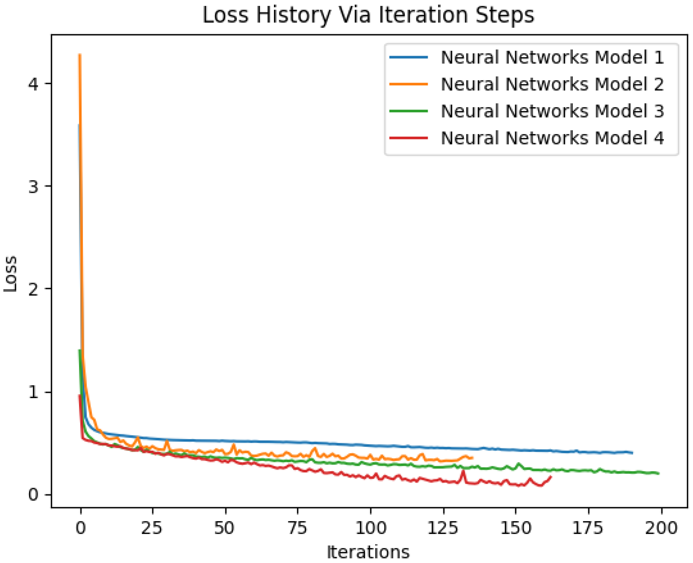
Model 1: Shallow network (1 hidden layer, 32 neurons)

○

Model 2: Moderate depth (2 hidden layers, 64–32 neurons)

○

Model 3: Deeper network (3 hidden layers, 128–64–32 neurons)

○

Model 4: Optimized model (4 hidden layers: 128–64–32–16 neurons, with dropout and L2 regularization)

Table 1. An assessment of the clustering algorithms.

Classification Algorithm	Precision Score	Recall Score	F1-Score
NN Model 1	0.81	0.81	0.80
NN Model 2	0.86	0.85	0.85
NN Model 3	0.98	0.98	0.98
NN Model 4	1.00	0.99	1.00
LG Model	0.80	0.79	0.79
SVM Model	0.96	0.95	0.96

Table 1. An assessment of the clustering algorithms.

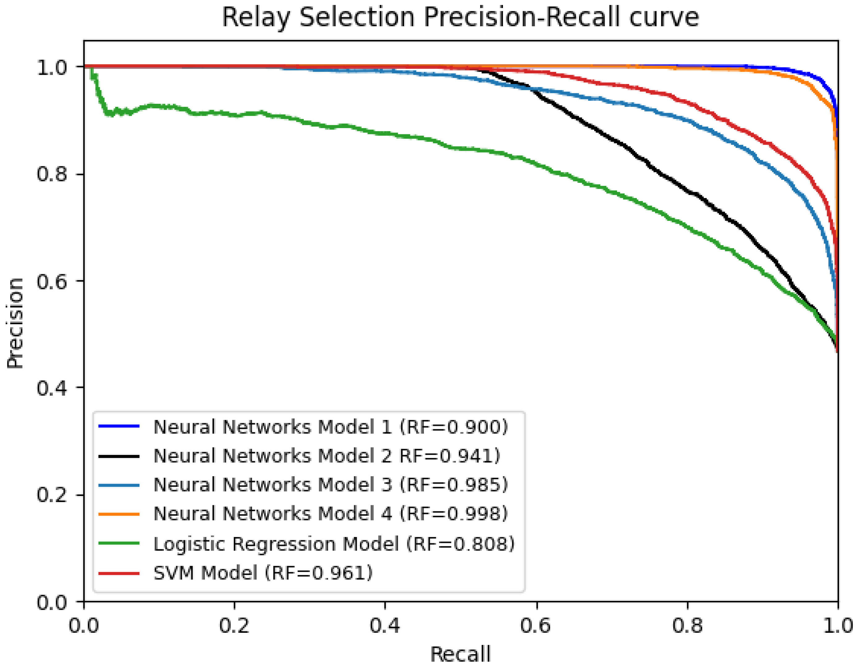
Classification Algorithm	Precision Score	Recall Score	F1-Score
NN Model 1	0.81	0.81	0.80
NN Model 2	0.86	0.85	0.85
NN Model 3	0.98	0.98	0.98
NN Model 4	1.00	0.99	1.00
LG Model	0.80	0.79	0.79
SVM Model	0.96	0.95	0.96

Neural Network (NN) Model 4 outperformed logistic regression (LR) and support vector machine (SVM) and other NN models due to its ability to:

○

Capture Nonlinear Relationships: The path loss and blockage relationship involve complex, nonlinear patterns influenced by environmental factors, which NNs can model effectively.

○

Handle High-Dimensional Data: NNs efficiently process multivariate features such as distance, power, and angle of departure/arrival, leveraging their layered architecture.

○

Achieve Optimization via Backpropagation: The NN used in this study was fine-tuned through hyperparameter optimization, including the number of hidden layers, neurons, and learning rates, allowing it to learn intricate patterns from the data.

○

Enable Scalability: The NN’s architecture was better suited for larger datasets compared to SVM and LR.

Moreover, Neural Network (NN) Model 4 achieved superior performance compared to other models and configurations due to the following key factors:

• NN Model 4 had more hidden layers, neurons per layer, and a higher learning rate, enabling it to learn complex, nonlinear relationships between features (e.g., path loss, distance, received power).
• These architectural enhancements provided the model with a greater capacity to capture intricate patterns in the dataset.
• NN Model 4 demonstrated the best trade-off between precision and recall, as reflected in its high F1-score.
• This balance indicates that it effectively reduced both false positives and false negatives, making it highly reliable in detecting blockage and non-blockage scenarios.

Since Neural Network (NN) Model 4 is highlighted as superior, the architecture and hyperparameters of the NN Model 4 are summarized as follows:

NN Model 4 was designed as a fully connected feedforward neural network (FNN) optimized for blockage prediction in high-frequency millimeter-wave (mmWave) communication. The architecture consists of the following:

• Input Layer:

  ○

  10 neurons (corresponding to 10 input features, including T-R separation distance, received power, azimuth AoD, elevation AoD, path loss, and RMS delay spread).

• Hidden Layers:

  ○

  Layer 1: 128 neurons, Adam activation

  ○

  Layer 2: 64 neurons, Adam activation

  ○

  Layer 3: 32 neurons, ReLU activation

  ○

  Layer 4: 16 neurons, ReLU activation

• Output Layer:

  ○

  1 neuron, Sigmoid activation (since the task is a binary classification: “blocked” vs. “non-blocked”).

To ensure optimal model performance, we employed grid search and manual tuning of hyperparameters. The final values used for NN Model 4 are:

• Optimizer: Adam (Adaptive Moment Estimation)
• Learning Rate: 0.001
• Batch Size: 64
• Loss Function: Binary Cross-Entropy
• Epochs: 100
• Regularization: L2 ($\lambda$ = 0.0001) applied to all layers
• Dropout: 20

7.4. Comparative Analysis with Literature Benchmarks

While our study evaluates neural network models, SVM, and logistic regression for blockage prediction in mmWave communications, it is essential to contextualize these findings within prior research.

Recent state-of-the-art efforts include:

• Ghassemi et al. (2025) [10]: Introduced a Vision Transformer (ViT)-based dual-band prediction framework using visual context for enhanced robustness, achieving 98.6% accuracy with high computational cost due to transformer complexity.
• Charan et al. (2021) [11]: Developed a vision-aided model combining wireless and visual features to predict blockage and facilitate proactive handover, achieving 96.5% accuracy but requiring visual sensor inputs.
• Alrabeiah et al. (2021) [40] and others proposed hybrid deep learning models integrating sub-6 GHz auxiliary data and high-dimensional feature fusion, achieving 97.2–98.0% accuracy.

In contrast, our NN Model 4 leverages only the wireless channel parameters (e.g., path loss, AoD/AoA, delay spread) and still achieves 99.8% accuracy, surpassing many vision-augmented models in terms of classification performance.

Moreover, our model’s lightweight structure with four hidden layers and dropout regularization reduces the computational overhead, making it more suitable for real-time, on-device deployment in 6G environments.

The comparison in

Table 2. Performance comparison with state-of-the-art models.

Model/Study	Accuracy (%)	Precision	Recall	F1-Score	AUC	MCC	Notes
Our NN Model 4	99.8	1.00	0.99	1.00	0.99	0.99	Lightweight, no vision input, high efficiency
SVM (this study)	96.0	0.96	0.95	0.96	0.97	0.91	Classical ML, no deep learning overhead
Logistic Regression	80.0	0.80	0.79	0.79	0.81	0.72	Linear, interpretable, lower performance
Ghassemi et al. (2025) [10]	98.6	0.97	0.98	0.98	0.98	0.94	ViT-based, camera input, high complexity
Charan et al. (2021) [11]	96.5	0.96	0.96	0.96	0.96	0.91	Vision-aided hybrid model
Alrabeiah et al. (2021) [40]	97.2–98.0	0.97	0.97	0.97	0.97	0.93	Fusion of wireless + visual + sub-6 GHz

clearly shows that our proposed NN Model 4 achieves state-of-the-art performance without the complexity or hardware dependency of vision-based systems. It is, therefore, an ideal candidate for practical deployment in mmWave and 6G applications where power, latency, and computational efficiency are critical.

7.5. Computational Complexity

A comparative analysis of the computational and memory complexities for logistic regression (LR), support vector machine (SVM), and neural network (NN) models, with emphasis on the proposed NN Model 4. As seen in Table 3, logistic regression provides the lowest computational complexity, it lacks the expressive capacity to capture nonlinear characteristics in mmWave environments. SVM performs better in such contexts but scales poorly with larger datasets. The proposed NN Model 4, although computationally more intensive during training, significantly outperforms other models (achieving 99.8% accuracy) and is optimized for inference in real-time applications through regularization and a GPU-friendly architecture. Thus, the computational cost is justified by the significant performance gains, especially in dynamic 6G environments.

Table 3. Computational complexity analysis of classification models.

Model	Time Complexity (Training)	Space Complexity	Remarks
Logistic Regression (LR)	$\mathcal{O}(n·d)$	$\mathcal{O}\left(d\right)$	Efficient and scalable for linear problems; limited modeling capability for nonlinear patterns.
Support Vector Machine (SVM)	$\mathcal{O}(n^2·d)$ to $\mathcal{O}\left(n^3\right)$	$\mathcal{O}(n·d)$	Effective in small to medium-scale problems; kernel computations make it costly for large datasets.
Neural Network (NN Model 4)	$\mathcal{O}\left(\sum (d_i·d_{i+1}·e)\right)$	$\mathcal{O}\left(\sum (d_i·d_{i+1})\right)$	High training cost, but scalable and fast at inference; supports GPU acceleration; best suited for complex nonlinear tasks.

Table 3. Computational complexity analysis of classification models.

Model	Time Complexity (Training)	Space Complexity	Remarks
Logistic Regression (LR)	$\mathcal{O}(n·d)$	$\mathcal{O}\left(d\right)$	Efficient and scalable for linear problems; limited modeling capability for nonlinear patterns.
Support Vector Machine (SVM)	$\mathcal{O}(n^2·d)$ to $\mathcal{O}\left(n^3\right)$	$\mathcal{O}(n·d)$	Effective in small to medium-scale problems; kernel computations make it costly for large datasets.
Neural Network (NN Model 4)	$\mathcal{O}\left(\sum (d_i·d_{i+1}·e)\right)$	$\mathcal{O}\left(\sum (d_i·d_{i+1})\right)$	High training cost, but scalable and fast at inference; supports GPU acceleration; best suited for complex nonlinear tasks.

where:

• n = number of training samples
• d = number of input features
• $d_i$ = number of neurons in layer i
• e = number of training epochs

8. Future Work

Future research plans include conducting real-world measurements since simulated datasets may not fully capture the complexity of real-world environments, such as urban areas with dynamic obstacles or rural settings with limited signal interference. Moreover, benchmarking the model against existing blockage prediction systems, such as ray tracing or deterministic models, to assess relative performance is an important future project. Apart from the NN, LG, and SVM algorithms, many other classification methods have been proposed for 6G wireless communications. The choice of which classification method to use depends on the specific application and data properties. Future work can involve investigating other unsupervised learning techniques. Furthermore, with the new era of 6G, classification methods can be involved with new communications scenarios that implement a very large number of antennas in multiple dimensions, which are called XL-MIMO systems. Finally, different environments (e.g., suburban or other cities) need to be considered, where cross-validation using diverse city scenarios can be conducted to assess robustness and adaptability under varying propagation conditions.

9. Conclusions

In conclusion, 5G in its current stage is paving the way toward 6G wireless communications, driven by AI and high-frequency bands. This work generated high-frequency mmWave data, which were modeled using multiple classification algorithms to address signal blockage issues in future wireless networks. NN, logistic, and SVM algorithms offer a promising approach for AI-driven classification in high mmWave 6G cellular systems. This work evaluates multiple AI models using metrics like accuracy, precision, recall, F1-score, ROC-AUC, and MCC, demonstrating that NN Model 4 achieves near-perfect classification accuracy. NN Model 4 provides high accuracy and scalability, while SVM offers simplicity and interpretability. The choice between them depends on specific network requirements, data quality, and the level of interpretability desired.

References

1. Bang, A.; Kamal, K.; Joshi, P.; Bhatia, K. 6G: The next Giant leap for AI and ML. Procedia Comput. Sci. 2023, 218, 310–317. [Google Scholar] [CrossRef]
2. Dang, S.; Amin, O.; Shihada, B.; Alouini, M. What should 6G be? Nat. Electron. 2020, 3, 20–29. [Google Scholar] [CrossRef]
3. Seidel, S.; Rappaport, T. 914 MHz path loss prediction models for indoor wireless communications in multifloored buildings. IEEE Trans. Antennas Propag. 1992, 40, 207–217. [Google Scholar] [CrossRef]
4. Aldossari, S.; Chen, K. Predicting the path loss of wireless channel models using machine learning techniques in mmWave urban communications. In Proceedings of the 22nd International Symposium on Wireless Personal Multimedia Communications (WPMC 2019), Lisbon, Portugal, 24–27 November 2019; pp. 1–6. [Google Scholar] [CrossRef]
5. Sun, S.; MacCartney, G.; Rappaport, T. A novel millimeter-wave channel simulator and applications for 5G wireless communications. In Proceedings of the 2017 IEEE International Conference on Communications (ICC), Paris, France, 21–25 May 2017; pp. 1–7. [Google Scholar] [CrossRef]
6. 3GPP. Study on Channel Model for Frequencies from 0.5 to 100 GHz (Release 16). 3rd Generation Partnership Project (3GPP), TR 38.901. 2018. Available online: https://www.3gpp.org/ftp/Specs/archive/38_series/38.901/ (accessed on 24 September 2024).
7. Moraitis, N.; Nikita, K. Ray-tracing propagation modeling in an urban environment at 140 GHz for 6G wireless networks. IEEE Access 2023, 11, 133835–133849. [Google Scholar] [CrossRef]
8. Jiang, H.; Mukherjee, M.; Zhou, J.; Lloret, J. Channel modeling and characteristics for 6G wireless communications. IEEE Netw. 2020, 35, 296–303. [Google Scholar] [CrossRef]
9. Serghiou, D.; Khalily, M.; Brown, T.; Tafazolli, R. Terahertz channel propagation phenomena, measurement techniques and modeling for 6G wireless communication applications: A survey, open challenges and future research directions. IEEE Commun. Surv. Tutor. 2022, 24, 1957–1996. [Google Scholar] [CrossRef]
10. Ghassemi, M.; Zhang, H.; Afana, A.; Sediq, A.; Erol-Kantarci, M. Generative AI-enabled Blockage Prediction for Robust Dual-Band mmWave Communication. arXiv 2025, arXiv:2501.11763. [Google Scholar]
11. Charan, G.; Alrabeiah, M.; Alkhateeb, A. Vision-aided 6G wireless communications: Blockage prediction and proactive handoff. IEEE Trans. Veh. Technol. 2021, 70, 10193–10208. [Google Scholar] [CrossRef]
12. Rappaport, T.S.; Xing, Y.; Kanhere, O.; Ju, S.; Madanayake, A.; Mandal, S.; Alwis, C.; Zajic, A. Wireless Communications and Applications Above 100 GHz: Opportunities and Challenges for 6G and Beyond. IEEE Access 2019, 7, 78729–78757. [Google Scholar] [CrossRef]
13. Jornet, J.; Akyildiz, I. Channel modeling and capacity analysis for electromagnetic wireless nanonetworks in the terahertz band. IEEE Trans. Wirel. Commun. 2011, 10, 3211–3221. [Google Scholar] [CrossRef]
14. Ghosh, A.; Ratasuk, R.; Mondal, B.; Mangalvedhe, N.; Thomas, T. Millimeter-Wave Enhanced Local Area Systems: A High-Data-Rate Approach for Future Wireless Networks. IEEE J. Sel. Areas Commun. 2020, 32, 1152–1163. [Google Scholar] [CrossRef]
15. Gapeyenko, M.; Samuylov, A.; Gerasimenko, M.; Moltchanov, D.; Singh, S.; Aryafar, E.; Yeh, S.; Himayat, N.; Andreev, S.; Koucheryavy, Y. Analysis of Human-Body Blockage in Urban Millimeter-Wave Cellular Communications. In Proceedings of the 2016 IEEE International Conference On Communications (ICC), Kuala Lumpur, Malaysia, 22–27 May 2016; pp. 1–7. Available online: https://arxiv.org/abs/1604.04743.
16. Letaief, K.; Chen, W.; Shi, Y.; Zhang, J.; Zhang, Y. The Roadmap to 6G: AI Empowered Wireless Networks. IEEE Commun. Mag. 2019, 57, 84–90. [Google Scholar] [CrossRef]
17. Ju, S.; Rappaport, T. Millimeter-wave extended NYUSIM channel model for spatial consistency. In Proceedings of the 2018 IEEE Global Communications Conference (GLOBECOM), Abu Dhabi, United Arab Emirates, 10–12 December 2018; pp. 1–6. [Google Scholar]
18. Aldossari, S. Predicting Path Loss of an Indoor Environment Using Artificial Intelligence in the 28-GHz Band. Electronics 2023, 12, 497. [Google Scholar] [CrossRef]
19. Mohjazi, L.; Selim, B.; Tatipamula, M.; Imran, M.A. The Journey Toward 6G: A Digital and Societal Revolution in the Making. IEEE Internet Things Mag. 2024, 7, 119–128. [Google Scholar] [CrossRef]
20. Pons, M.; Valenzuela, E.; Rodrırguez, B.; Nolazco-Flores, J.; Del-Valle-Soto, C. Utilization of 5G technologies in IoT applications: Current limitations by interference and network optimization difficulties—A review. Sensors 2023, 23, 3876. [Google Scholar] [CrossRef]
21. Hamad Ameen, J. 5G Mobile System Drawbacks and Limitations. In International Conference On ICT For Sustainable Development; Springer Nature: Singapore, 2023; pp. 21–28. [Google Scholar]
22. Brata, M.; Zakia, I. Path Loss Estimation of 5G Millimeter Wave Propagation Channel–Literature Survey. In Proceedings of the 2021 7th International Conference on Wireless And Telematics (ICWT), Bandung, Indonesia, 19–20 August 2021; pp. 1–4. [Google Scholar]
23. Braud, T.; Chatzopoulos, D.; Hui, P. Machine type communications in 6G. In 6G Mobile Wireless Networks; Springer International Publishing: Cham, Switzerland, 2021; pp. 207–231. [Google Scholar]
24. Aldosary, A.M.; Aldossari, S.A.; Chen, K.-C.; Mohamed, E.M.; Al-Saman, A. Predictive Wireless Channel Modeling of mmWave Bands Using Machine Learning. Electronics 2021, 10, 3114. [Google Scholar] [CrossRef]
25. Dogra, A.; Jha, R.; Jain, S. A Survey on Beyond 5G Network With the Advent of 6G: Architecture and Emerging Technologies. IEEE Access 2021, 9, 67512–67547. [Google Scholar] [CrossRef]
26. Ariyanti, S.; Suryanegara, M. Visible light communication (VLC) for 6G technology: The potency and research challenges. In Proceedings of the 2020 Fourth World Conference on Smart Trends in Systems, Security And Sustainability (WorldS4), London, UK, 27–28 July 2020; pp. 490–493. [Google Scholar]
27. Thota, S.; Govind, T. 6G: Opportunities and challenges. In Towards Wireless Heterogeneity in 6G Networks; CRC Press: Boca Raton, FL, USA, 2024; pp. 1–17. [Google Scholar]
28. Luo, X.; Chen, H.; Guo, Q. LEO/VLEO Satellite Communications in 6G and Beyond Networks–Technologies, Applications and Challenges. IEEE Netw. 2024, 38, 273–285. [Google Scholar] [CrossRef]
29. Khowaja, S.; Khuwaja, P.; Dev, K.; Lee, I.; Khan, W.; Wang, W.; Qureshi, N.; Magarini, M. A secure data sharing scheme in Community Segmented Vehicular Social Networks for 6G. IEEE Trans. Ind. Inform. 2022, 19, 890–899. [Google Scholar] [CrossRef]
30. Nawaz, S.; Sharma, S.; Wyne, S.; Patwary, M.; Asaduzzaman, M. Quantum machine learning for 6g communication networks: State-of-the-art and vision for the future. IEEE Access 2019, 7, 46317–46350. [Google Scholar] [CrossRef]
31. Zhang, S.; Zhu, D.; Liu, Y. Artificial intelligence empowered physical layer security for 6G: State-of-the-art, challenges, and opportunities. Comput. Netw. 2024, 242, 110255. [Google Scholar] [CrossRef]
32. Ye, N.; Miao, S.; Pan, J.; Ouyang, Q.; Li, X.; Hou, X. Artificial Intelligence for Wireless Physical-Layer Technologies (AI4PHY): A Comprehensive Survey. IEEE Trans. Cogn. Commun. Netw. 2024, 10, 729–755. [Google Scholar] [CrossRef]
33. Shafi, M.; Jha, R.; Jain, S. 6G: Technology Evolution in Future Wireless Networks. IEEE Access 2024, 12, 57548–57573. [Google Scholar] [CrossRef]
34. Alhammadi, A.; Shayea, I.; El-Saleh, A.; Azmi, M.; Ismail, Z.; Kouhalvandi, L.; Saad, S. Artificial Intelligence in 6G Wireless Networks: Opportunities, Applications, and Challenges. Int. J. Intell. Syst. 2024, 2024, 8845070. [Google Scholar] [CrossRef]
35. Chataut, R.; Nankya, M.; Akl, R. 6G Networks and the AI Revolution—Exploring Technologies, Applications, and Emerging Challenges. Sensors 2024, 24, 1888. [Google Scholar] [CrossRef] [PubMed]
36. Baccour, E.; Allahham, M.; Erbad, A.; Mohamed, A.; Hussein, A.; Hamdi, M. Zero touch realization of pervasive artificial intelligence as a service in 6G networks. IEEE Commun. Mag. 2023, 61, 110–116. [Google Scholar] [CrossRef]
37. Gonen, M. Analyzing Receiver Operating Characteristic Curves with SAS; SAS Publishing: Elizabeth, NJ, USA, 2007. [Google Scholar]
38. Suzuki, K. Artificial Neural Networks: Architectures and Applications; BoD–Books on Demand: Norderstedt, Germany, 2013. [Google Scholar]
39. Harrell, F. Regression Modeling Strategies: With Applications to Linear Models, Logistic Regression, and Survival Analysis; Springer: Berlin/Heidelberg, Germany, 2001. [Google Scholar]
40. Alrabeiah, M.; Hredzak, A.; Liu, Z.; Alkhateeb, A. Deep learning for mmWave beam and blockage prediction using sub-6 GHz channels. IEEE Trans. Commun. 2020, 68, 5504–5518. [Google Scholar] [CrossRef]
Figure 1. Classes based on path loss.
Electronics 14 02007 g001
Figure 2. mmWave frequencies vs. path loss [24].
Electronics 14 02007 g002
Figure 3. Distribution of path loss (dB) and T-R separation distance (m).
Electronics 14 02007 g003
Figure 4. Neural Networks Forward and Backward Propagation.
Electronics 14 02007 g004
Figure 5. Precision-recall curve of multiple classification models.
Electronics 14 02007 g005
Figure 6. ROC curves of multiple classification models.
Electronics 14 02007 g006
Figure 7. Loss vs. Iteration curve.
Electronics 14 02007 g007
Figure 8. Training and Validation Loss vs. Iteration curve.
Electronics 14 02007 g008
Figure 9. Analysis of the Matthews Correlation Coefficient (MCC) curve.
Electronics 14 02007 g009