Heterogeneous Multi-Sensor Fusion for AC Motor Fault Diagnosis via Graph Neural Networks

Abstract

Multi-sensor fault diagnosis, especially when using heterogeneous sensors, substantially enhances the accuracy of fault detection in asynchronous motors operating under high-interference conditions. A critical challenge in multi-sensor fault diagnosis lies in effectively fusing data from different sensors. Deep learning offers a promising solution by transforming multi-sensor data into a unified representation, thereby facilitating robust data fusion. However, existing approaches often fail to fully exploit inter-sensor correlations and inherent prior physical knowledge. To address this limitation, we propose a novel graph neural network-based model that emphasizes graph structure construction for heterogeneous multi-sensor information fusion. Our framework includes (1) a multi-task enhanced autoencoder for node feature extraction, enabling discriminative representation learning, particularly with heterogeneous sensor data; (2) an adjacency matrix builder integrated with physical prior constraints to improve the generalization and robustness of the model; and (3) a graph isomorphism network to derive graph-level representations for fault classification. Our experimental results demonstrate the model’s effectiveness in diagnosing faults, as it achieves superior performance compared to conventional methods on two heterogeneous asynchronous motor datasets.

1. Introduction

With the advantages of a high energy conversion rate, durability, and low cost, asynchronous motors (AC motors) play an important role in industrial equipment. These motors are the primary drivers in machinery such as conveyors, pumps, and grinders, which are prone to faults due to their harsh operating environments and complex working conditions [1]. Implementing fault diagnosis technology for motors is essential to ensuring the reliability, safety, and efficiency of the overall system. The early detection and accurate identification of faults enable timely maintenance, preventing catastrophic failures and ensuring optimal performance. Consequently, research on AC motor fault diagnosis has garnered significant attention [2].

Effective fault diagnosis in AC motor systems requires the installation of sensors to monitor critical operational parameters. The key parameters to monitor include temperature, vibration, acoustic emissions, current, voltage, and electromagnetic field. Although vibration-based models have demonstrated high accuracy in bearing fault diagnosis [3], the complexity of motor systems often renders single-sensor data inadequate for making a reliable diagnosis. For instance, vibration signals may be affected by long propagation paths, which result in noise contamination and coupled vibration components that obscure a fault’s characteristics [4]. The integration of multi-sensor data into diagnostics addresses these limitations by providing a comprehensive health assessment of a system, reducing measurement errors, and improving diagnostic accuracy through the fusion of complementary information. Furthermore, multi-sensor systems exhibit greater resilience to environmental interference and noise, ensuring more stable and reliable diagnostic outcomes. This approach enables multi-level, multi-angle analyses, making it particularly suitable for complex systems. Recent studies have consistently demonstrated the superiority of multi-sensor methods in the fault diagnosis of various types of rotating machinery, including motors, gearboxes, and pumps [5,6,7].

To effectively leverage multi-sensor data for fault detection, a robust multi-source fusion method must capture inter-sensor correlations and interactions. Fusion can occur at three levels: the data [8], feature, and decision level [9,10,11]. Among these three, feature-level fusion is the predominant approach, as it generates a shared representation that maximizes correlation information. Early feature-level fusion methods primarily relied on statistical techniques, which assume specific probability distributions for sensor data and estimate the joint distributions of fused features. Methods such as principal component analysis (PCA) [12], linear discriminant analysis (LDA) [13], and independent component analysis (ICA) [14] have demonstrated success in fault diagnosis. However, these approaches suffer from computational complexity with high-dimensional data and performance degradation when the real data deviate from the assumed distributions.

Recent advances in deep learning have enabled us to create end-to-end models that automatically extract and integrate fault-sensitive features from multi-sensor data. Since sensor data typically consist of 1D time series (which can be transformed into 2D representations) [15,16], convolutional neural networks (CNNs) are well suited to hierarchical feature extraction. Consequently, CNNs and their variants have been widely adopted for multi-sensor fusion. Further improvements have been achieved by combining CNNs with recurrent neural networks (RNNs), attention mechanisms, and residual networks [17,18,19]. For instance, Wang et al. [20] developed an attention-based multidimensional CNN for multi-modal feature fusion, significantly improving diagnostic accuracy. Hao et al. [21] integrated a 1D-CNN with LSTM to capture spatiotemporal features, demonstrating its robustness in low signal-to-noise ratio scenarios. Xie et al. [22] enhanced CNNs with residual connections for deployment on image-like multi-signal data, achieving high accuracy with low computational overhead. Other architectures, including deep Boltzmann machines [23], autoencoders [24], transfer learning [25], and capsule networks [26], have also been explored to further advance the diagnosis of faults.

While the aforementioned network models implicitly leverage complementary information from multiple sensors, graph neural networks (GNNs) provide an explicit framework for modeling inter-sensor correlations through graph-based representations. In this paradigm, nodes represent sensors while edges encode their relationships, enabling a comprehensive analysis of both local and global patterns. Recent years have witnessed the growing adoption of GNNs in fault diagnosis, with numerous studies demonstrating their effectiveness in this domain. Wang et al. [27] developed an attention-based temporal–spatial GNN (A-TSGNN) that combines graph convolution with temporal learning to capture spatiotemporal features while using attention mechanisms to weigh sensor importance. This approach achieved a robust performance across multiple datasets. Xu et al. [28] proposed a graph-guided collaborative CNN (GGCN) that addresses signal distribution discrepancies while exploiting intrinsic multi-source correlations, demonstrating strong noise immunity in electromechanical systems. Wang et al. [29] integrated GNNs with Markov transition fields (MTFs); the MTFs preserve temporal correlations in 2D signal representations while graph attention networks (GATs) dynamically adjust node weights, leading to high accuracy under noisy and variable load conditions. Duan et al. [30] introduced DyGAT-FTNet, which features an automatic adjacency matrix constructed from STFT time–frequency features through a learnable dynamic graph mechanism that is enhanced by integrated spatiotemporal dependency extraction. Wang et al. [31] developed a densely connected spatiotemporal GNN that combines graph diffusion convolution with pooling operations, effectively capturing the complex spatiotemporal dependencies in rotating machinery.

Recent studies have demonstrated GNNs’ effectiveness in fault diagnosis and how they have led to innovations in spatiotemporal modeling, dynamic graph learning, and attention-based weighting. Despite these advances, a critical research gap remains—existing GNN-based methods rely heavily on pre-defined or simplistic graph constructions, neglecting two key challenges: (1) Inadequate node feature extraction. Current approaches use raw sensor segments [27,31], time–frequency features [29,30], or basic CNN-extracted representations [28], which fail to account for sensor heterogeneity or noise susceptibility. This limits discriminative feature learning, particularly in systems with diverse sensor modalities. (2) Over-reliance on data-driven adjacency matrices. Most methods create adjacency matrices using data only, ignoring prior physical knowledge (e.g., sensor placement, system dynamics). This leads to poor generalization in noisy or data-scarce scenarios.

To overcome these limitations, this paper proposes a multi-task enhanced autoencoder for node feature extraction. By leveraging the representation learning capabilities of autoencoders, we introduced auxiliary tasks that enable the model to learn the discriminative features related to different types of sensors. For adjacency matrix construction, we combined data-driven methods with prior physical knowledge to improve generalization and robustness, particularly in noisy or data-scarce conditions. The resulting graph data were processed using a graph isomorphism network (GIN) to capture spatial features, which is followed by a stacked readout mechanism that generates a unified representation for fault classification. Experiments on two novel heterogeneous multi-sensor datasets validate the proposed model’s superior performance.

The main contributions of this study are summarized as follows:

(1)

Multi-Task Enhanced (MTE) Autoencoder for Feature Extraction: This module is designed to learn discriminative feature representations, particularly within heterogeneous sensor data. By combining the representation learning capability of autoencoders with two auxiliary tasks—an anomaly detection task to enhance feature discriminability for fault diagnosis and a sensor-type classification task to embed sensor-specific information—the module improves feature robustness. The encoder architecture is able to extract multi-scale features using a CNN and self-attention mechanism, optimizing its effectiveness in processing vibration and current signals from AC motor systems.

(2)

Physics-Informed Adjacency Matrix Construction: By incorporating data-driven correlation learning and the physical constraints from sensor configurations, an adjacency matrix builder is established for the connections between nodes. This hybrid approach improves both the generalization capability and noise robustness of the resulting graph representations.

(3)

GIN-Based Diagnostic Framework: We have developed an end-to-end fault diagnosis system that uses a GIN for node information aggregation and stacking readouts for effective graph-level feature learning. This framework achieves a state-of-the-art performance on new heterogeneous multi-sensor datasets, demonstrating its strong generalizability.

The structure of this paper is organized as follows: Section 2 introduces related background theories. Section 3 details the proposed model. Section 4 validates the proposed method using heterogeneous multi-sensor AC motor datasets. Finally, Section 5 concludes the paper.

2. Preliminaries

2.1. Problem Definition

Suppose S sensors are installed in an AC motor system to collect data for status monitoring and fault diagnosis. A sample of the monitoring data would consist of S time series. Assuming each sensor measures the same length of data for T, the data from the i-th sensor can be represented as the time series $X_i=\{x_{i,1},x_{i,2},\dots ,x_{i,T}\}$. Thus, one sample from all the input data can be denoted as $X=\{X_1,X_2,\dots ,X_S\}$. The label for the fault state of each data sample can be derived from expert knowledge or predefined manual settings, which are represented as $Y\in \{{Fault}_1,{Fault}_2,\dots ,{Fault}_C\}$, where C is the total number of fault categories possible. The problem lies in developing an intelligent fault diagnosis model F that classifies fault types based on multi-sensor signal measurements:

$$Y=F\left(X\right),X\in R^{S\times T}$$

(1)

where X is the input multi-sensor data and Y is the output fault type.

2.2. Multi-Sensor Signals for Fault Diagnosis

The types of signals sensors capture play a crucial role in the design of fault diagnosis schemes. For AC motors, the most critical signals to measure are vibration and current signals. Consider bearing faults, one of the most common issues in rotating machinery (Figure 1). When defects form in the inner or outer ring due to fatigue, inner or outer ring failure occurs. As rolling elements periodically pass through the defect zone, the bearing generates a series of impulse responses. These responses introduce characteristic fault frequencies in the frequency domain, such as Ball Pass Frequency Outer (BPFO) and Ball Pass Frequency Inner (BPFI) races. The resulting signal is a modulation of entry and exit events, which can be expressed as follows:

$$X_{vib}=\sum _{n}g\left(t\right)\delta \left(t-n/f_c\right)$$

(2)

where $g\left(t\right)$ is the impulse response function, which depends on defected surface topography, and $\delta \left(t\right)$ is the impulse with a characteristic vibration frequency $f_c$, which is determined by the bearing’s geometry and rotational speed. The characteristic frequencies of the inner ring, outer ring, and rolling element can be mathematically expressed as follows:

$$f_{ci}={\displaystyle \frac{N{f}_r}{2}}\left(1+{\displaystyle \frac{d}{D}}cos\phi \right)$$

(3)

$$f_{co}={\displaystyle \frac{N{f}_r}{2}}\left(1-{\displaystyle \frac{d}{D}}cos\phi \right)$$

(4)

$$f_{co}={\displaystyle \frac{D{f}_r}{d}}\left(1-({\displaystyle \frac{d}{D}}cos\phi {)}^2\right)$$

(5)

where N denotes the number of rolling balls; fr denotes the rotational speed; d is the rolling element diameter; D is the pitch circle diameter; and $\phi$ is the contact angle of the bearing.

When a bearing failure occurs in an AC motor, the resulting mechanical displacement modifies the air gap, leading to corresponding changes in the current components. These variations in current are influenced by both the vibration frequency and the supply frequency of the motor. Consequently, the failure introduces fluctuations into the supply current, which can be expressed as follows:

$$X_{cur}=Asin\left(2\pi f_{s}t\right)h\left(t\right)$$

(6)

where $f_s$ denotes the supply frequency and $h\left(t\right)$ denotes the current variations caused by bearing faults. The characteristic frequency of a bearing fault in the current signal is denoted as follows:

$$f_{bf}=\left|f_s\pm k{f}_{cx}\right|$$

(7)

where $f_{cx}$ denotes the characteristic vibration frequency of the bearing fault.

The aforementioned analysis includes a vibration analysis (VA) and motor current signature analysis (MCSA), which are pivotal technologies used in motor fault diagnosis and have achieved considerable success [2,32]. These methods encompass time-domain statistical analyses, spectral analyses, and time–frequency analyses. In deep learning-based approaches, they are often employed as feature extraction techniques. However, this study diverges from these conventional methods, instead adopting an autoencoder-based framework. The design of our encoding process is nevertheless inspired by these traditional feature extraction techniques.

2.3. Background to the GNN

Since a sample of the multi-sensor data are a collection of time series, this time series must be converted into graph-structured data before being processed by a GNN model. Graph-structured data have a non-Euclidean data structure that consists of nodes and edges. Nodes represent entities (i.e., sensors) and edges represent their relationships. Mathematically, a graph structure can be represented as $G=\{V,E\}$, where $V$ is the set of nodes and $E$ is the set of edges, which indicate the connections between nodes. Each node is associated with a feature, which is denoted as $Z$. The structure of the graph, which depicts the dependencies between nodes, is defined by the adjacency matrix as follows:

$$A_{nm}=\left\{\begin{array}{c} 1,if\left(v_n,v_m\right)\in E\\ 0, otherwise\hfill \end{array}\right.$$

(8)

Each element of the adjacency matrix indicates the presence of an edge between a node pair. The matrix $A_{nm}$ can be modified to account for the strength of these relationships:

$$A_{nm}=\left\{\begin{array}{cc}{w}_{nm},& if\left(v_n,v_m\right)\in E\\ 0,& otherwise\end{array}\right.$$

(9)

Traditional deep learning models like CNNs and RNNs cannot be directly applied to graph data due to the data’s irregular structure. GNNs overcome this limitation by learning graph representations through message aggregation between nodes, which gives them significant advantages in diverse domains such as multi-sensor systems, social networks [33], and transportation systems [34].

The information contained in each node is determined by its own features and the features of its neighbors. The goal of a GNN is to learn a state embedding vector, which contains information about the node and its neighbors, for each node. The message aggregation process can be described as follows:

$$h_n^{\left(t+1\right)}=\sum _{k\in N\left(n\right)}{M}_t\left(z_n^t,z_k^t,A_{nk}\right)$$

(10)

$$z_n^{\left(t+1\right)}=U_t\left(z_n^t,h_n^{\left(t+1\right)}\right)$$

(11)

where $h_n^{(t+1)}$ and $z_n^{(t+1)}$ are the updated messages and node states at step t + 1, $M$ is the message function, $A_{nk}$ represents the element of the adjacency matrix, $N\left(n\right)$ denotes the neighbors of the node, and $U_t$ is the node update function.

By using stacking or pooling strategies for the nodes, GNNs convert graph-structured data into a canonical representation, making them easier to process with various neural networks. GNNs have achieved excellent results in tasks such as node classification, edge prediction, graph clustering, and graph classification. After turning multi-sensor data into graph data, the fault diagnosis problem can be framed as a graph classification task.

3. Proposed Method

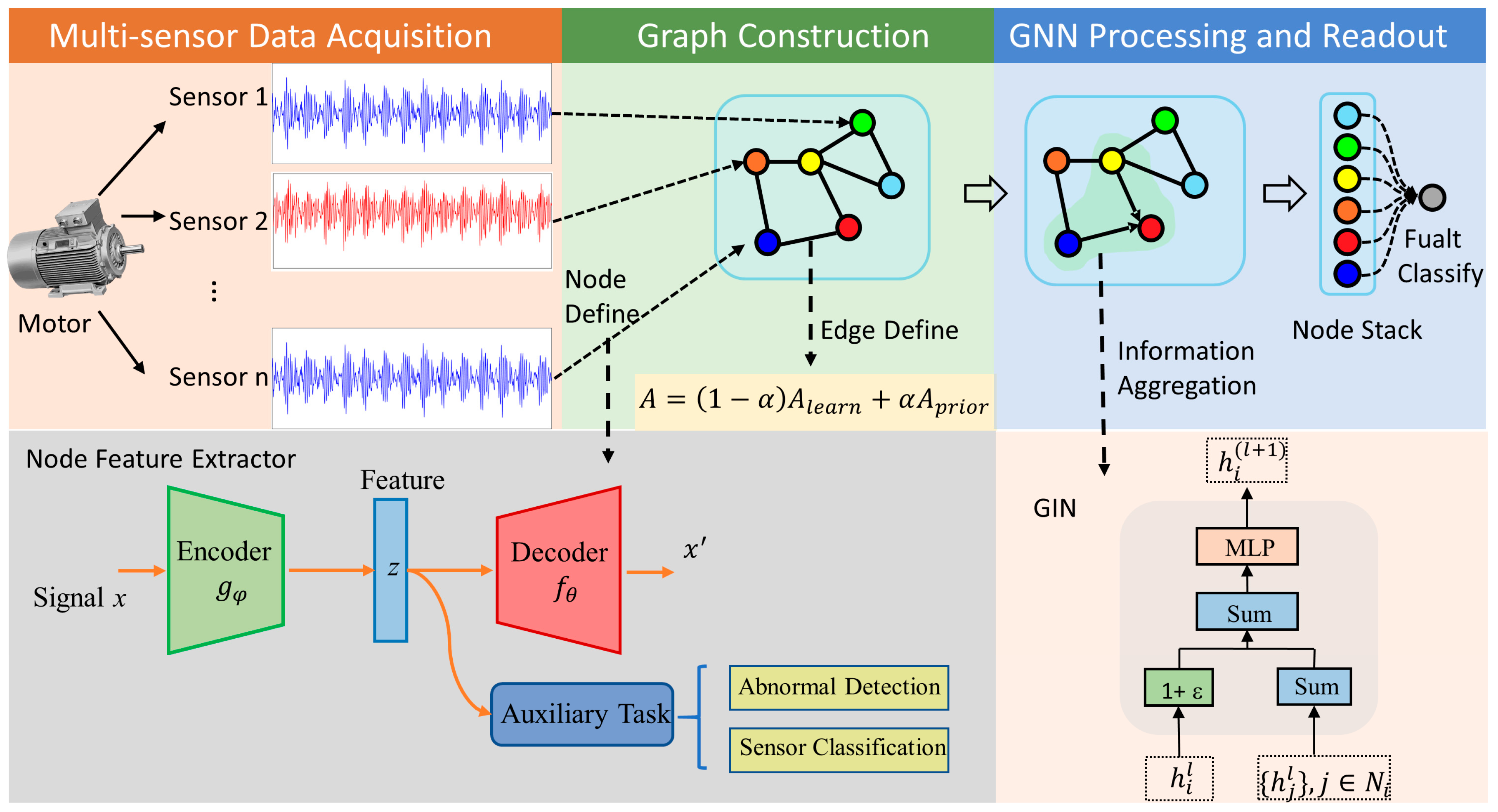
3.1. Overview of Model Architecture

The framework of our proposed model, as illustrated in Figure 2, comprises three key stages:

(1)

Multi-sensor Data Acquisition

This stage involves the synchronous or asynchronous acquisition of system state information from heterogeneous sensors (e.g., vibration, temperature, or current sensors) and the conversion of raw physical signals into processable digital data. The objective is to enable comprehensive system monitoring via multi-source perception, providing a robust foundation of data for downstream tasks such as fault diagnosis or health assessments.

(2)

Graph Construction

Using that multi-sensor data a graphical representation of the data are created, which includes the following:

Node Definition: Features are extracted from the sensor data using a multi-task enhanced autoencoder. This architecture combines the autoencoder’s feature extraction capability with two auxiliary tasks to improve its discriminability, particularly when working with heterogeneous sensor data.

Edge Definition: An adjacency matrix is constructed to model the interdependencies between sensors. This matrix integrates data-driven correlations with physical prior constraints (e.g., the spatial proximity or functional coupling of sensors) to enhance interpretability and robustness.

(3)

GNN Processing and Graph Readout

The constructed graph is processed via a GIN, which was selected for its ability to identify non-isomorphic graphs while maintaining computational efficiency. The GIN captures the spatial correlations among sensors, after which a readout module generates a graph-level representation. This representation is transformed into a diagnostic output through a stacked, fully connected, multi-layer network.

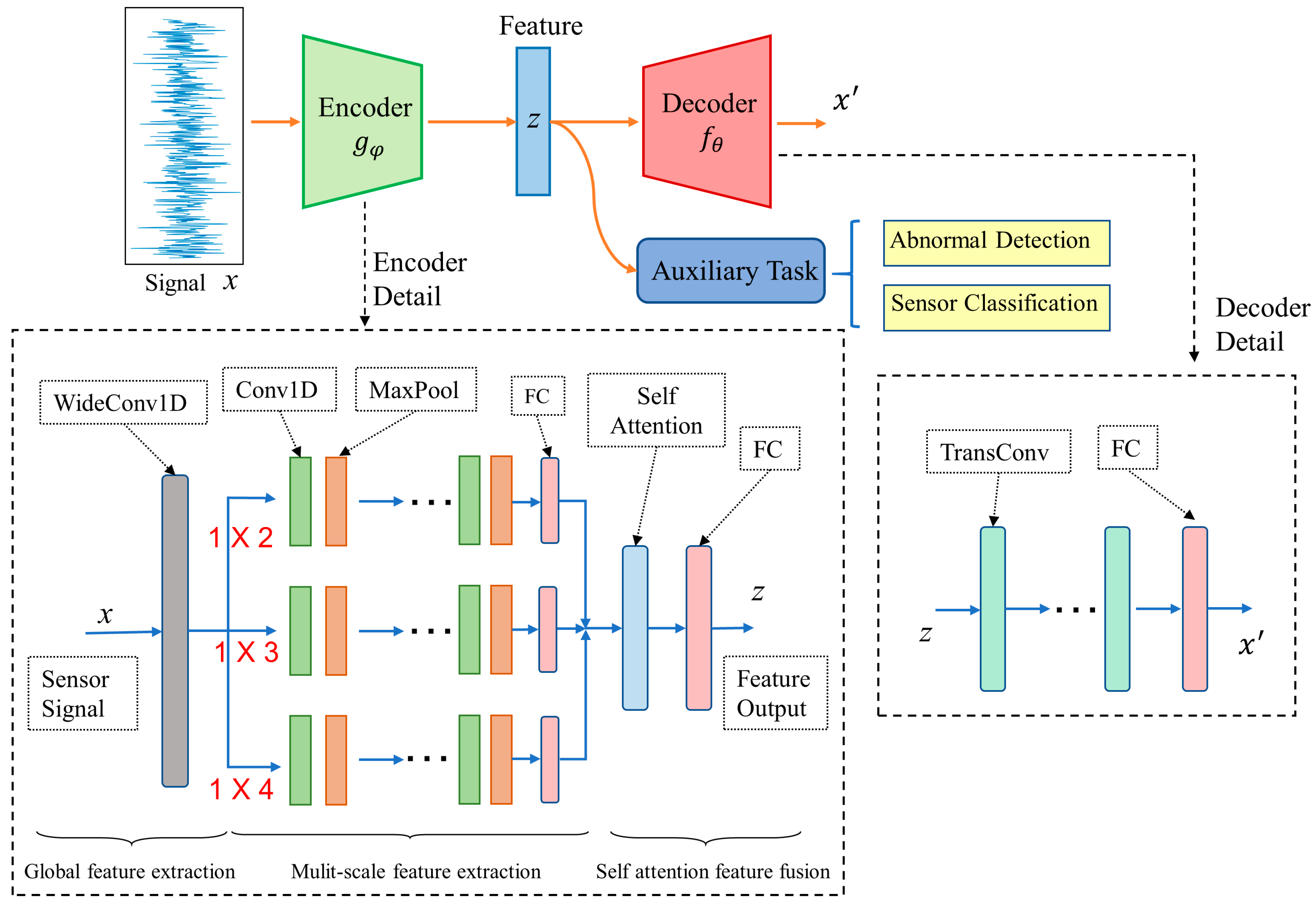
3.2. Multi-Task Enhanced Autoencoder for Feature Extraction

3.2.1. General Framework for Node Extractor

A node feature extractor is designed to convert raw signals into dense vector representations. We use an autoencoder framework, consisting of an encoder $g_{\phi }$ and a decoder $f_{\theta }$, as the node feature extractor in our model, as illustrated in Figure 3.

Given an input time series sample x, the encoder compresses the data into a dense representation z as follows:

$$z=g_{\phi }\left(x\right)$$

(12)

The decoder then reconstructs the data from the dense feature representation z as follows:

$$x^{\prime }=f_{\theta }\left(z\right)$$

(13)

Through this information bottleneck, a low-dimensional representation is learned by minimizing the reconstruction loss as follows:

$$L_{recstr}={\displaystyle \frac{1}{N}}\sum _{i=1}^N{\left(x_i-{x_i}^{\prime }\right)}^2$$

(14)

While the information bottleneck helps filter out noise and redundancy, it may overlook information relevant to fault diagnosis if no additional constraints are used. For instance, if the current signal is a sine waveform of the supply frequency that is superimposed by variations caused by a bearing fault, although the sine waveform constitutes the main part of the signal, it is irrelevant to the fault (Figure 1). To address this problem, we propose two auxiliary tasks that ensure the encoder retains fault-relevant information: an abnormal detection task and a sensor-type classification task. These tasks leverage readily available labels for healthy/faulty states and sensor types during data collection. The abnormal detection task takes feature z as its input and outputs a prediction of $\widehat{y}$ by minimizing the binary cross-entropy loss function as follows:

$$L_{abn}={\displaystyle \frac{1}{N}}\sum _{i=1}^N-y_{i}log{\widehat{y}}_i+\left(1-y_i\right)log\left(1-{\widehat{y}}_i\right)$$

(15)

where $y_i,{\widehat{y}}_i\in \{healthy,faulty\}$ are the true and predicted labels, respectively. This task encourages the encoder to extract features that better distinguish between healthy and faulty conditions.

The sensor-type classification task takes feature z as its input and predicts the sensor type by minimizing the cross-entropy loss function as follows:

$$L_{sens}={\displaystyle \frac{1}{N}}\sum _{i=1}^N\sum _{j=1}^C-y_{ij}log{\widehat{y}}_{ij}$$

(16)

where $y_{ij},{\widehat{y}}_{ij}\in \{S_1,S_2,\dots ,S_C\}$ are the true and predicted labels for C sensor types, created using one-hot encoding. This task embeds sensor information into the node features, aiding in subsequent graph edge definition. The overall loss function is as follows:

$$L_{total}=L_{recstr}+L_{abn}+L_{sens}$$

(17)

where $L_{recstr}$ is the reconstruction loss, $L_{abn}$ is the abnormal detection loss, and $L_{sens}$ is the sensor-type classification loss.

3.2.2. Multi-Scale CNN Encoder

The network model of the encoder significantly impacts the effectiveness of the feature extractor. The successful application of wavelet transforms [35] and empirical mode decomposition (EMD) [36] in vibration signal analysis highlights the importance of global and multi-scale local feature extraction [37]. Inspired by these approaches, we propose a combination of global and multi-scale local feature extraction to obtain robust features from time series data based on a CNN. We combined the CNN with an attention mechanism to better suit our feature extraction goals for multi-sensor data, as illustrated in Figure 3. First, a wide convolution operation is applied to create a global feature representation of the raw signal:

$$f_w=Conv\left(X_i,WideKer\right)$$

(18)

where $X_i$ is the input sensor signal and $WideKer$ denotes the wide convolution kernel, which is set to 1 × 64 to capture long-term correlations in lengthy time series. The convolution operation for a 1D signal is expressed as follows:

$$Conv\left(x,ker\right)=\sum _{n}x\left(n\right)ker\left(m-n\right)$$

(19)

To acquire hierarchical feature representations, we designed a multi-scale CNN module to extract rich features at multiple scales. This module consists of several branches of CNNs, each comprising multiple convolution operations with different kernel sizes and a MaxPool operation. The different kernel sizes are used to extract multi-scale features. The number of branches is a hyper-parameter and is set to 3 in our model. This process is expressed as follows:

$$\left\{\begin{array}{c}M{f}_1=MaxPool\left(Conv\left(f_w,1\times 2\right)\right)\\ M{f}_2=MaxPool\left(Conv\left(f_w,1\times 3\right)\right)\\ M{f}_3=MaxPool\left(Conv\left(f_w,1\times 4\right)\right)\end{array}\right.$$

(20)

After extracting the multi-scale features, they are fused using a self-attention layer to extract the most relevant information. The fused features are then compressed using a fully connected (FC) layer as follows:

$$z=FC\left(Attn\left(M{f}_1,M{f}_2,M{f}_3\right)\right)$$

(21)

The self-attention layer and FC layer can be expressed as follows:

$$Attn\left(\left(K,V\right),Q\right)=Softmax\left({\displaystyle \frac{Q\otimes K^T}{\sqrt{d_k}}}\right)V$$

(22)

$$FC\left(x\right)=f\left(Wx+b\right)$$

(23)

where Q is the query vector, K is the key vector, V is the value vector, ⊗ denotes the dot product, W is the weight matrix, b is the bias term, and f is the activation function. The softmax function converts the output of the neural network into a probability distribution and is defined as follows:

$$Softmax\left(z\right)={\displaystyle \frac{e^{z_i}}{{\sum }_i{e}^{z_i}}}$$

(24)

3.2.3. Transposed CNN-Based Decoder

The decoder is designed with multiple layers of transposed convolution and with padding, which is used to reconstruct the input data while maintaining the information flow’s symmetry. The final layer is an FC layer with the same length as the input sequence:

$$x^{\prime }=FC\left(TransConv\left(z\right)\right)$$

(25)

where $x^{\prime }$ represents the reconstructed data. Transposed convolution works by inserting zeros (or other padding values) between the input feature maps and then performing convolution on the expanded input using the same filters as in standard convolution.

For the auxiliary tasks, both of which are classification tasks, we used multiple FC layers, with a softmax output, as the predictor. These two tasks share a similar network architecture, which can be expressed as follows:

$$y=Softmax\left({FC}_m\left(z\right)\right)$$

(26)

where y is the label given to the abnormal detection task or the sensor-type classification task; ${FC}_m\left(z\right)$ denotes multiple FC layers.

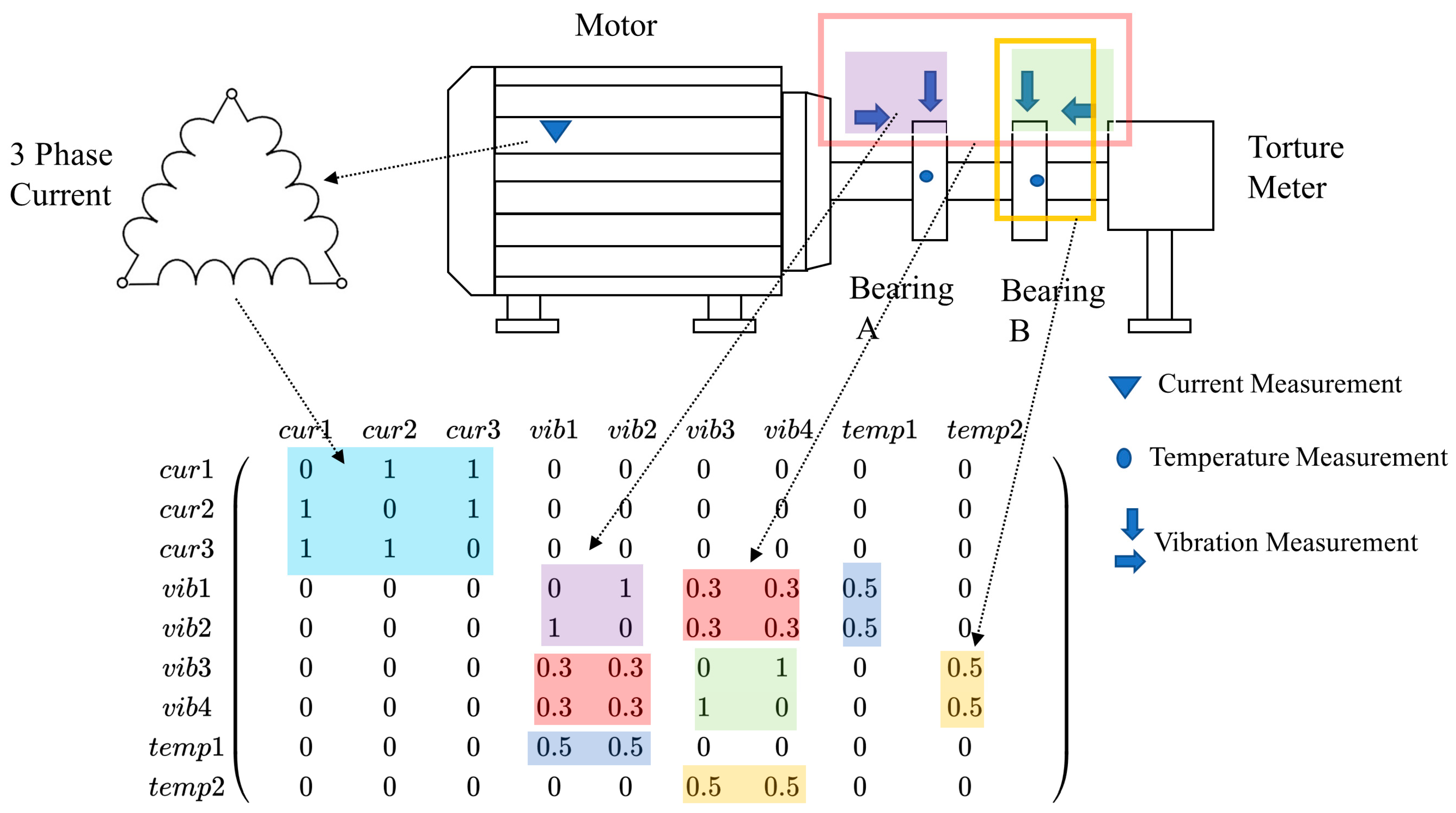
3.3. Adjacent Matrix Builder with Physical Constraint

Given the node features extracted from each sensor, a data-driven approach can be used to construct the adjacency matrix. However, purely data-driven methods are often vulnerable to data bias and noise. To mitigate these limitations, we propose a hybrid method that integrates prior knowledge of the sensor configuration with data-driven techniques to improve graph construction. The most common data-driven approach for adjacency matrix construction is the metric-based method, which defines a metric function to measure pairwise node distances. First, we compute the adjacency matrix $A_{learn}$ using the Pearson correlation coefficient as the metric function. Each element of $A_{learn}$ is calculated as follows:

$$A_{nm}={\displaystyle \frac{{\sum }_{i=1}^d\left(z_{n,i}-{\overline{z}}_m\right)\left(z_{m,i}-{\overline{z}}_n\right)}{\sqrt{{\sum }_{i=1}^d{\left(z_{n,i}-{\overline{z}}_n\right)}^2}\sqrt{{\sum }_{i=1}^d{\left(z_{m,i}-{\overline{z}}_m\right)}^2}}}$$

(27)

where ${\overline{z}}_m$ and ${\overline{z}}_n$ represent the mean values of the node features $z_n$ and $z_m$, respectively. All elements of $A_{learn}$ are normalized to the range [0, 1].

Inspired by [38], which encodes prior knowledge of the physical connections between motor components, we introduced a prior-knowledge adjacency matrix $A_{prior}$. To account for the consistency and similarity of fault-related information in sensor data, we assigned different connection weights: a weight of 1 is assigned to data from the same type of sensors within the same component, as they contain the most similar fault-related information; a weight of 0.5 is assigned to data from different sensors within the same component; a weight of 0.3 is assigned to sensors in different components that are joined by a signal transmission path. For example, vibration sensors measuring different bearings are assigned a weight of 0.3 due to potential signal coupling, whereas temperature sensors remain unconnected due to their slow dynamics and mutual independence (see Figure 4). The weight factor is empirically determined; however, when combined with the adjustable hyperparameter α, introduced later, it facilitates the construction of a well-structured adjacency matrix.

The two matrices are then fused linearly using the weighting coefficient $\alpha$:

$$A_{fuse}={\left(1-\alpha \right)A}_{learn}+\alpha A_{prior}$$

(28)

The resulting $A_{fuse}$ is a weighted adjacency matrix. To retain the most significant connections, we use the top-k nearest neighbors (tKNNG) method [39], which preserves only the K strongest node pairs based on their weights.

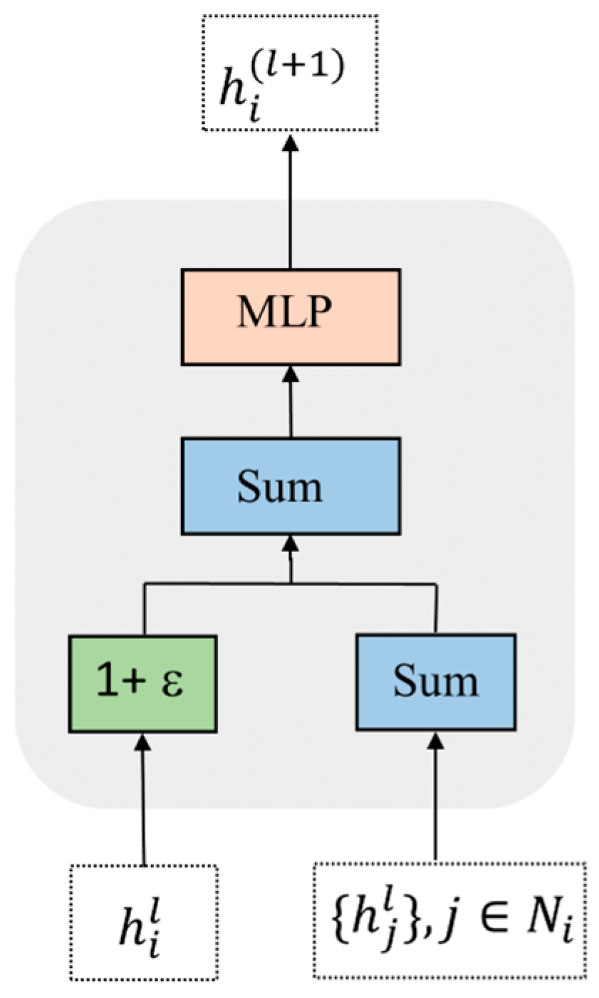
3.4. GIN Processing and Readout

To effectively capture sensor correlations through the constructed graph, we employed a GIN model, as introduced by Xu et al. [40]. The core idea of a GIN is to update node features through sum aggregation and multi-layer perceptrons (MLPs), enabling the capture of subtle differences in graph structures. Unlike traditional GNN models, such as Graph Convolutional Networks (GCNs) and graph attention networks (GATs), a GIN utilizes a summation operation to aggregate neighbor information instead of mean or max operations. As illustrated in Figure 5, the node feature update at layer l is as follows:

$$h_i^{\left(l+1\right)}={MLP}^l\left(\left(1+{\epsilon }^l\right)·h_i^l+\sum _{j\in N_i}{h}_j^l\right)$$

(29)

where $h_i^l$ denotes the feature representation of node i in layer l, $N_i$ represents the set of nodes that neighbor node i, ${\epsilon }^l$ is a learnable parameter used to adjust the importance of the node’s own features, and ${MLP}^l$ refers to the multi-layer perceptron used for nonlinear transformations.

After the nodes have updated the information from their neighbor nodes for a number of rounds, a readout method is implemented to derive a holistic graph-level representation of the features of all nodes. We use stacking method for this purpose. First, all node features are stacked into a vector as follows:

$$H_{stack}=h_1^{\prime }⨁h_2^{\prime }⨁\dots ⨁h_N^{\prime }$$

(30)

Next, an FC layer is applied to obtain a graph-level representation as follows:

$$H_{graph}=FC\left(H_{stack}\right)$$

(31)

Finally, an FC network, followed by a softmax function, is used to classify the fault type:

$$Y=Softmax\left(FC\left(H_{graph}\right)\right)$$

(32)

4. Experiments

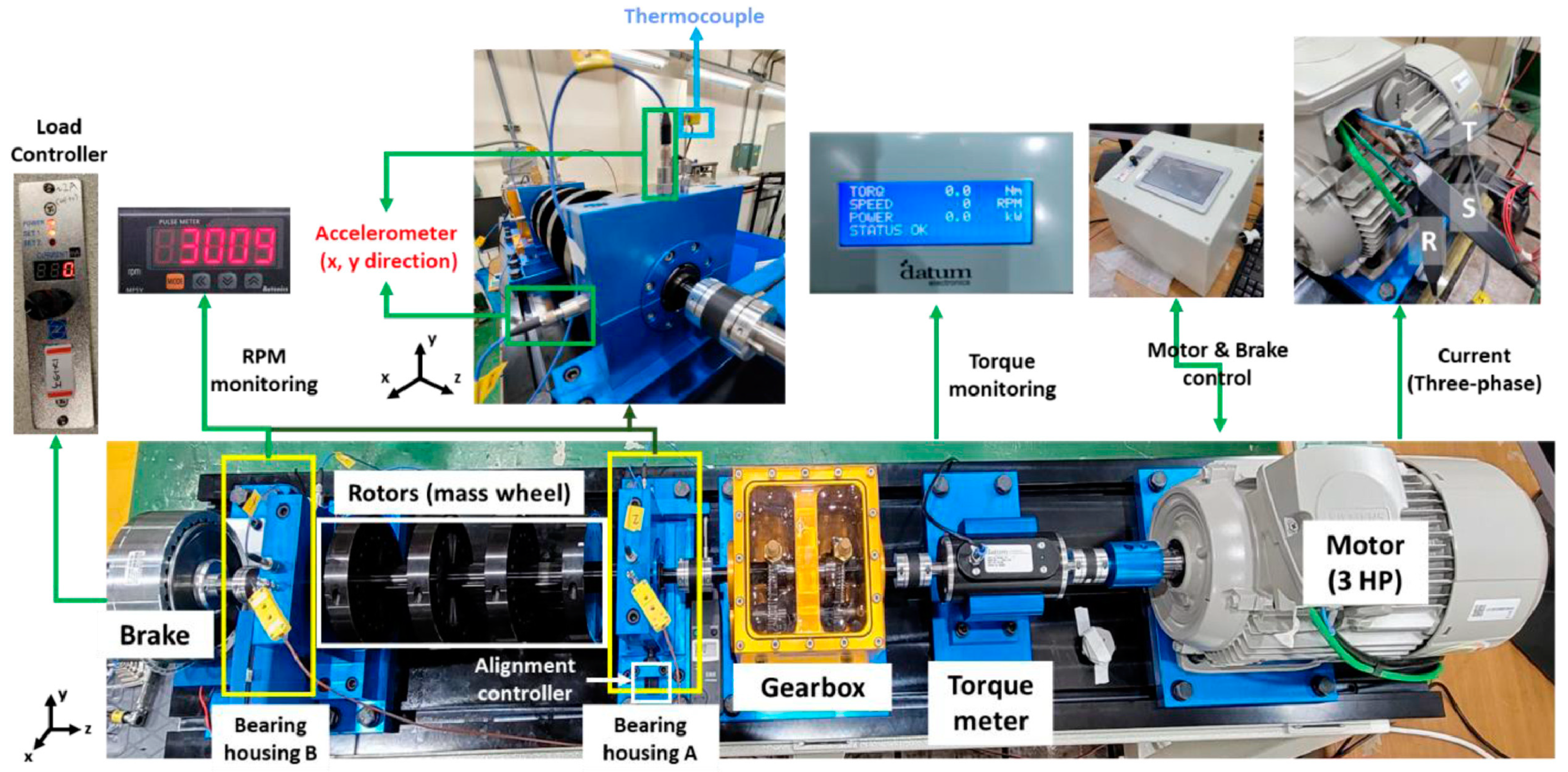
4.1. Dataset Description

To evaluate the model’s performance, we selected two publicly available heterogeneous multi-sensor datasets to use as benchmarks: vibration, acoustic, temperature, and motor current dataset (VATMCD) [41] and University of Ottawa Electric Motor Dataset (UOEMD) [42].

The VATMCD was collected from an AC motor testbed that features a 380 V/60 Hz three-phase induction motor coupled with a torque meter, gearbox, two NSK bearings (labeled A and B), multiple rotors, and a hysteresis brake (Figure 6). The system includes ten sensors that monitor critical parameters (

Table 1. Sensor configurations in VATMCD and UOEMD.

Dataset	Sensor	Data Type	Model	Quantity	Location	Load Condition	Sample Rate (kHz)
VATMCD	Accelerometers	Vibration	PCB35234	4	Bearing A&B (x,y)	0, 2, 4 (Nm)	25.6
	Thermocouples	Temperature	PCB378B02	2	Bearing A&B	0, 2, 4 (Nm)	25.6
	Microphones	Acoustic	K-type	1	Near bearing A	0 (Nm)	51.2
	Current Sensors	Current	Hioki CT6700	3	Motor	0, 2, 4 (Nm)	25.6
UOEMD	Accelerometers	Vibration	PCB623C01	3	Motor drive, Bearing L&R	Loaded, Unloaded	42
	Thermocouples	Temperature	PCB603C01	1	Motor drive	Loaded, Unloaded	42
	Microphones	Acoustic	PCB 130F20	1	Near bearing L	Loaded, Unloaded	42

). Acoustic data were only recorded under no-load conditions and were excluded from our experiments. The testbed replicates four fault conditions: inner race bearing faults, outer race bearing faults, the parallel misalignment of shafts, and rotor unbalance.

The UOEMD consists of heterogeneous multi-sensor data collected from a customized Spectra Quest Machinery Fault and Rotor Dynamics Simulator. The setup includes a 380 V/60 Hz three-phase motor mounted on vibration-damped rubber supports, a variable-frequency drive, and two 6205-series bearings (labeled L and R). Five sensors monitored the system in both its loaded and unloaded state (Table 1). The dataset encompasses seven fault conditions: rotor unbalance, rotor misalignment, stator winding faults, voltage unbalance and single phasing, a bowed rotor, broken rotor bars, and bearing faults.

4.2. Data Preprocessing and Model Training

Each data record was scaled to fit the range of [0, 1] using min–max normalization, which was calculated as follows:

$$\overline{x}={\displaystyle \frac{x-x_{min}}{x_{max}-x_{min}}}$$

(33)

To generate the dataset, we employed the non-overlapped method with a window length of 4096 samples to ensure the integrity of the fault events. The VATMCD comprises 27,000 samples in total, and each sample is represented as a 9 × 4096 matrix, where 9 corresponds to the number of sensors used. The UOEMD comprises 6656 samples in total and each sample is represented as a 5 × 4096 matrix. The datasets were randomly split into training and test sets in an 8:2 ratio. To maximize the use of the training data and improve the model’s generalization ability, we performed 5-fold cross-validation on the training set. It is important to note that the same split was applied to each fault type and across all loads.

Due to differences in the configurations of the sensors in the VATMCD and UOEEMD datasets, the models were trained separately. However, some of their modules shared the same hyperparameters. The hyperparameters of the models are detailed in

Table 2. Hyperparameter settings.

Module	Hyperparameter	Value
Node Feature Extractor	Number of CNN layers in each encoder branch	3
	Self-attention input dimension	64
	Number of self-attention heads	3
	Encoder output dimension	32
	Number of transposed convolution layers	4
	Number of MLP layers for auxiliary task	3
	Batch size	32
	Training epochs	100
	Learning rate	0.001
Adjacent Matrix Builder	Weighting factor of physical prior constraints	0.4/0.4 *
	Number of retained edges	20/7 *
GIN	Number of hidden layers	4
	Batch size	32
	Training epochs	100
	Learning rate	0.001

* Hyperparameter corresponding to the VATMCD and UOEEMD datasets.

. All experiments were implemented in PyTorch 1.13.1 on Python 3.9.13 (computational infrastructure used: Ubuntu 22.04 operating system, CPU Intel 12400K, GPU NVIDIA RTX 3070).

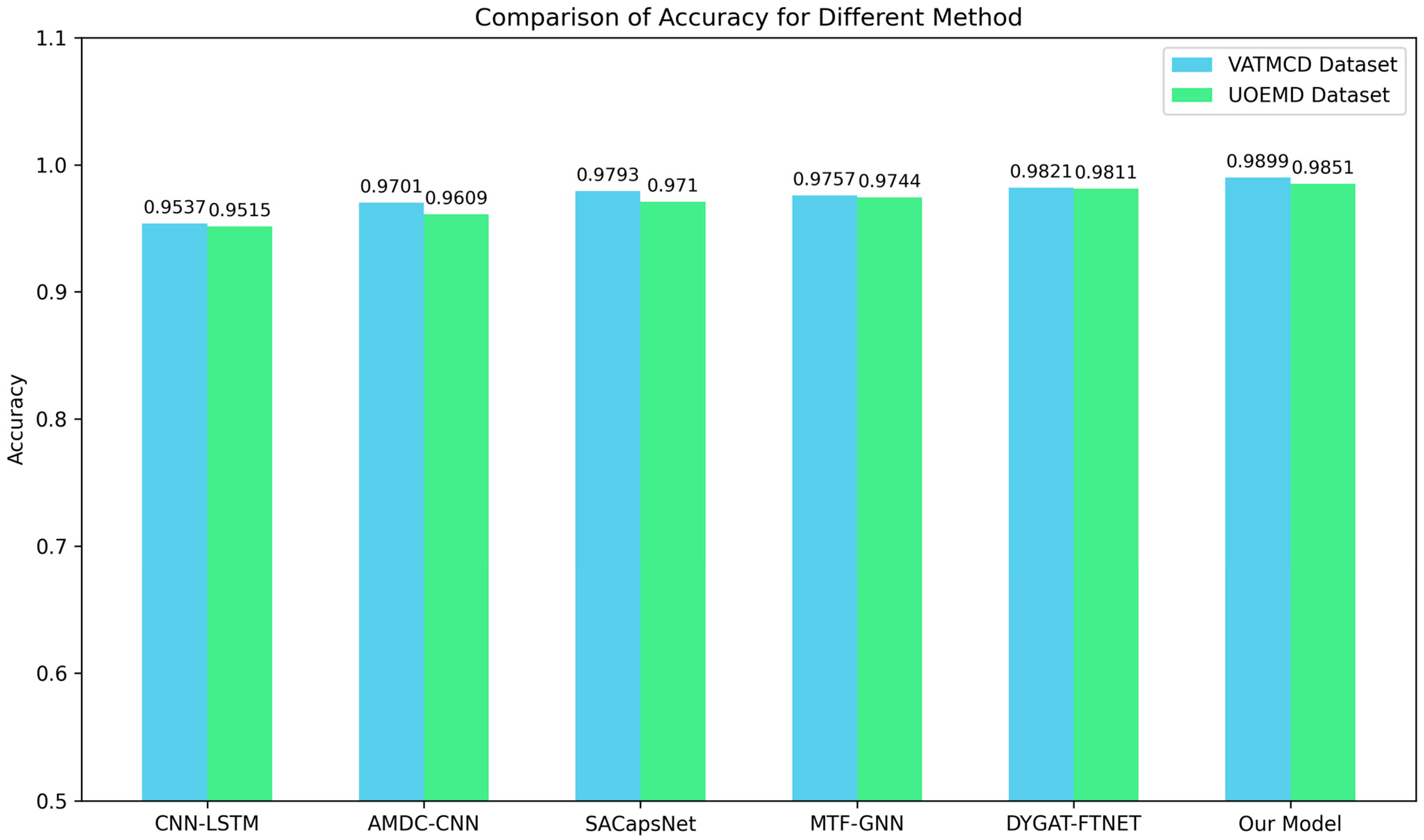
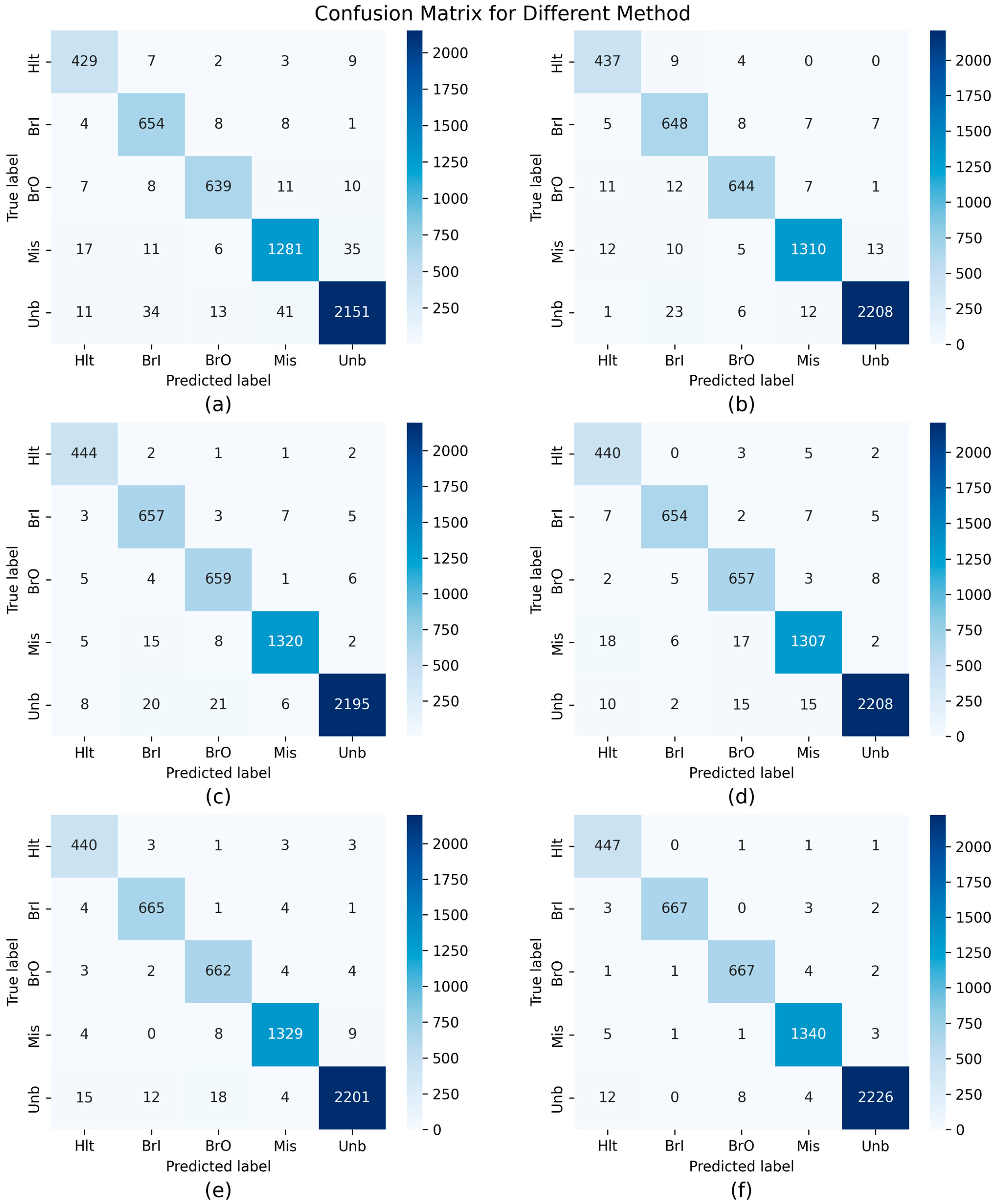
4.3. Comparative Experiment

To evaluate the effectiveness of our proposed model, we conducted a comparative experiment against several state-of-the-art multi-sensor fault diagnosis models, namely CNN-LSTM [21], AMDC-CNN [20], SACapsNet [26], MTF-GNN [29], and DYGAT-FTNET [30]. Each of these models was meticulously reproduced by following the parameters specified in their respective publications during both the training and testing phases. Minor adjustments were made to accommodate the test dataset, as some models were originally evaluated on homogeneous multi-sensor datasets. To ensure robustness and minimize the impact of randomness, each experiment was repeated five times. To ensure a fair comparison, all models were evaluated using the same dataset and the training methodology outlined in Section 4.2, as well as identical training hyperparameters (e.g., epoch count and batch size). The performance of the models was assessed using mean accuracy and macro F1 score, which are defined as follows:

$$Acc={\displaystyle \frac{TP+TN}{TP+TN+FP+FN}}$$

(34)

$$F1={\displaystyle \frac{1}{C}}\sum _{i=1}^C{F1}_i={\displaystyle \frac{1}{C}}\sum _{i=1}^{C}2{\displaystyle \frac{{Precision}_i\times {Recall}_i}{{Precision}_i+{Recall}_i}}$$

(35)

where TP, TN, FP, and FN represent true positive, true negative, false positive, and false negative instances, respectively. C is the number of fault classes, and ${Precision}_i$ and ${Recall}_i$ are the precision and recall of the model for each fault class and defined as follows:

$$Precision={\displaystyle \frac{TP}{TP+NP}}$$

(36)

$$Recall={\displaystyle \frac{TP}{TP+FN}}$$

(37)

The experimental results, summarized in

Table 3. Comparative experimental results.

Method	VATMCD		UOEMD
	Accuracy	F1 Score	Accuracy	F1 Score
CNN-LSTM	0.9537	0.9434	0.9515	0.9514
AMDC-CNN	0.9701	0.9623	0.9609	0.9609
SACapsNet	0.9793	0.9751	0.9710	0.9708
MTF-GNN	0.9757	0.9697	0.9744	0.9743
DYGAT-FTNET	0.9821	0.9772	0.9811	0.9809
Our Model	0.9899	0.9878	0.9851	0.9850

and visualized in Figure 7, demonstrate the superior performance of our proposed model over other methods. Its performance on the VATMCD is consistently higher than on the UOEMD, which can be attributed to the VATMCD’s larger sample size and greater number of sensors per sample.

Additionally, we created a confusion matrix for each method’s performance on the VATMCD to highlight their specific strengths and weaknesses in fault classification. As shown in Figure 8, both our method and DYGAT-FTNET model achieved classification accuracies exceeding 98%. However, some models exhibited notable limitations in identifying specific fault types. For instance, CNN-LSTM showed a high misclassification rate for shaft misalignment faults, while AMDC-CNN frequently misclassified shaft misalignment faults as a healthy state. These shortcomings may stem from the models’ inability to effectively differentiate between similar signals and leverage the relevant information available from the multi-sensor data.

4.4. Analysis of MTE Node Feature Extractor

This section presents a comparative analysis of our MTE node feature extractor, which was carried out over two experimental studies. Only the VATMCD was utilized was this analysis.

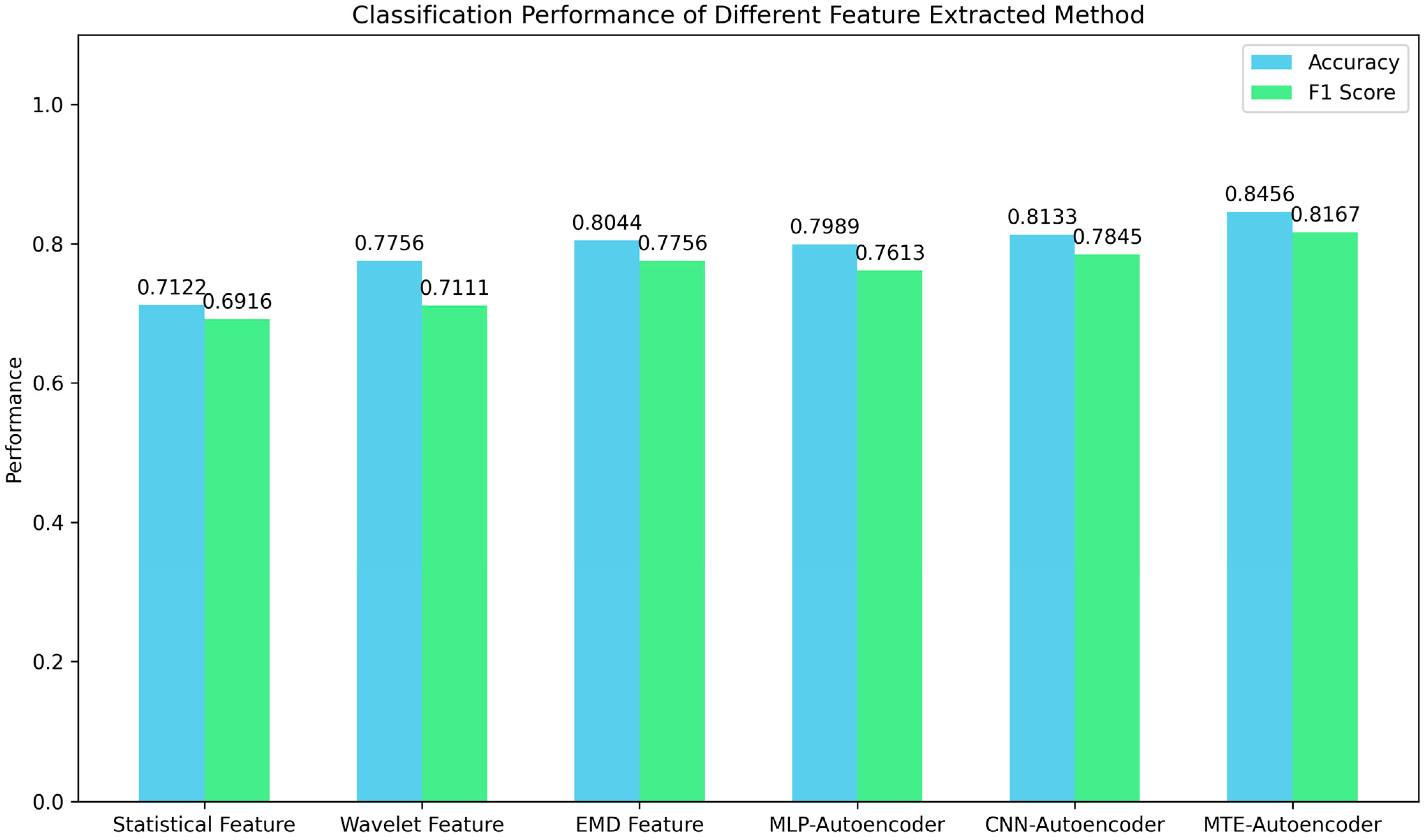
4.4.1. Comparative Study of Different Feature Extraction Methods

To evaluate the performance of different feature extraction methods, we conducted comparative experiments to assess how our proposed MTE node feature extractor measured up against three conventional handcrafted approaches and two encoder-based methods. The experimental configuration used in this study is detailed in

Table 4. Comparison of experimental methods and configurations.

Method	Description
Statistical Feature-Based Model	A total of 16 time-domain and frequency-domain statistical features including the mean amplitude, root mean square, square mean root, peak value, peak-to-peak value, variance, standard deviation, waveform factor, kurtosis coefficient, skewness coefficient, frequency center, mean frequency, frequency variance, mean standard frequency, frequency ratio, and standard deviation frequency.
Wavelet Feature-Based Model	Signal decomposition using db4 wavelet with three decomposition levels (yielding eight sub-bands). Four features (mean, root mean square, energy ratio, and kurtosis) were extracted from each sub-band, resulting in 24-dimensional feature vectors.
EMD Feature-Based Model	Empirical mode decomposition produced eight intrinsic mode functions (IMFs), with four features (mean, root mean square, energy ratio, and kurtosis), per IMF, yielding 24-dimensional feature vectors.
MLP Autoencoder	Four-layer MLP encoder and decoder architecture with 32-dimensional representation of latent space.
CNN Autoencoder	Four-layer CNN encoder and transposed CNN decoder architecture with 32-dimensional representation of latent space.
Multi-task Enhanced Autoencoder	Architecture as described in Section 3.2, with 32-dimensional representation of latent space.

. The three autoencoder-based models were trained for 100 epochs. For each multi-sensor data sample, we extracted features from individual sensors using these methods, concatenated the resulting features, and processed them through a four-layer MLP network for fault classification. We evaluated each feature extraction approach based on its classification accuracy and F1 score, training the MLP network for 50 epochs in each case.

The experimental results (Figure 9) demonstrate that autoencoder-based feature extraction methods generally outperform conventional approaches. Notably, the basic MLP autoencoder underperformed relative to the EMD method, suggesting that simple network architectures may not effectively capture the complex patterns present in multi-sensor data for fault diagnosis. Among the autoencoder-based methods tested, CNN architectures benefit from their inherent structural constraints, while the MTE autoencoder achieves a superior performance through additional imposed constraints. These findings indicate that with sufficient training data, properly constrained autoencoders can develop robust feature extraction capabilities. Furthermore, our results suggest that simple MLP classifiers may not effectively leverage multi-sensor information for optimal fault diagnosis, even when well-extracted features are provided.

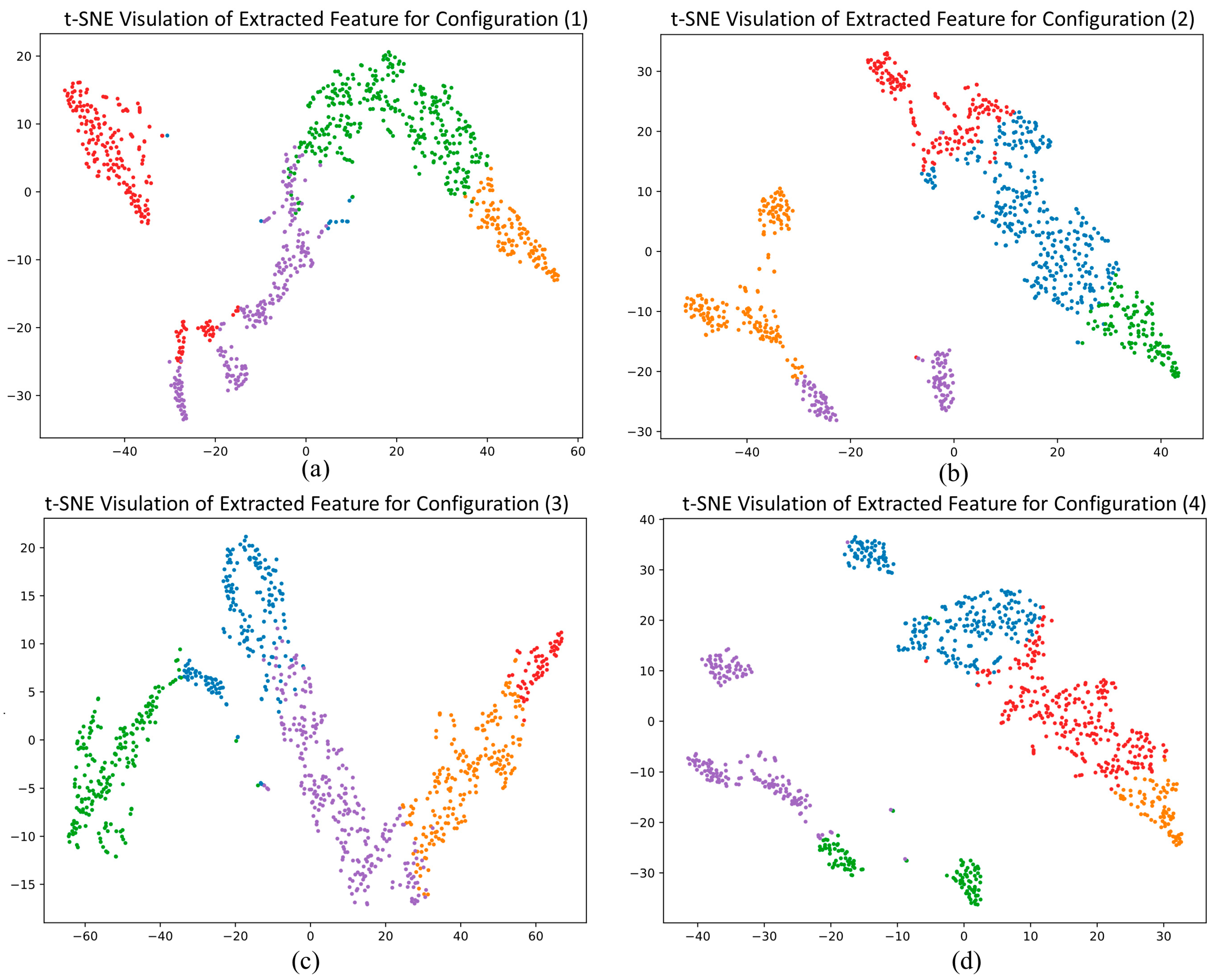
4.4.2. Comparative Study of Different Task Combinations

The MTE node feature extractor uses two auxiliary tasks to enhance its feature extraction performance. To evaluate their effectiveness, we conducted experiments that used the autoencoder’s signal reconstruction task as the baseline framework, assessing their ability to discriminate between node feature representations under different auxiliary task combinations. Specifically, we examined four configurations: (1) reconstruction only, (2) reconstruction with anomaly detection, (3) reconstruction with sensor-type classification, and (4) reconstruction with both auxiliary tasks. All experiments employed identical network architectures and training hyperparameters, with early stopping implemented to mitigate overfitting.

We evaluated the discriminability of the extracted node representations using Gaussian Mixture Models (GMM) clustering, a probabilistic clustering method that is particularly suitable for complex data distributions. The performance of the extractor was quantified using three established metrics: the Silhouette Index (SI), Calinski–Harabasz Index (CHI), and Davies–Bouldin Index (DBI). The Silhouette Index is defined as follows:

$$SI={\displaystyle \frac{1}{n}}\sum _{i=1}^n{\displaystyle \frac{b\left(x_i\right)-a\left(x_i\right)}{max\left(b\left(x_i\right),a\left(x_i\right)\right)}}$$

(38)

where $a\left(x_i\right)$ represents the average distance between a sample and all other samples within the same cluster $C_i$ and $b\left(x_i\right)$ denotes the minimum average distance between $x_i$ and the samples in other clusters.

The Calinski–Harabasz Index is defined as follows:

$$CHI={\displaystyle \frac{\left(\sum _{i=1}^k{n}_i{‖c_i-c‖}^2\right)/\left(k-1\right)}{\left(\sum _{i=1}^k\sum _{x_i\in C_i}{‖x_i-c‖}^2\right)/\left(n-k\right)}}$$

(39)

where n is the total number of samples, k is the number of clusters, $n_i$ is the number of samples in $C_i$, $c_i$ is the centroid of $C_i$, and c is the centroid of the entire dataset.

The Davies–Bouldin Index is defined as follows:

$$DBI={\displaystyle \frac{1}{k}}\sum _{i=1}^k{max}_{j\ne i}\left({\displaystyle \frac{S_i+S_j}{d\left(c_i,c_j\right)}}\right)$$

(40)

where $S_i$ represents the average distance between each sample in cluster $C_i$ and its centroid $c_i$.

The experimental results, presented in

Table 5. Clustering results of the node features.

Configurations	SI	CHI	DBI
(1) Reconstruction alone	0.3914	1030.62	0.8891
(2) Reconstruction with abnormal detection	0.4736	1202.06	0.8695
(3) Reconstruction with sensor-typeclassification	0.4063	1153.18	0.8809
(4) Reconstruction with both abnormal detection and sensor-type classification	0.5195	1610.89	0.8519

and visualized via t-distributed Stochastic Neighbor Embedding (t-SNE) in Figure 10, demonstrate that the anomaly detection task substantially improves the discrimination of node features. In comparison, the sensor-type classification task provides only a modest enhancement. Nevertheless, the sensor information obtained remains useful for edge definition, despite showing limited impact in this specific experimental context.

4.5. Noise Resistance

To assess the noise robustness of our model, we conducted experiments evaluating its diagnostic performance under varying levels of noise. Gaussian noise ranging from −10 dB to 10 dB was systematically introduced to raw sensor data from both datasets. The trained models then performed fault diagnosis on the noise-contaminated data, with their classification accuracy serving as the evaluation metric.

The experimental results (Figure 11) demonstrate that our model exhibits strong noise resilience within moderate noise ranges, preserving its high accuracy (>95%) at 10 dB and 5 dB signal-to-noise ratios. However, its performance degrades with increasing noise amplitudes. Our comparative analysis reveals it has a greater sensitivity to noise in the UOEMD, which we attribute to the dataset’s lower sensor count (five sensors/sample versus nine in VATMCD). This difference highlights the importance of redundant sensors for ensuring noise robustness in fault diagnosis systems.

4.6. Hyperparameter Sensitivity Analysis

We conducted a sensitivity analysis using the VATMCD to evaluate how the hyperparameters affect the model’s performance and to determine their optimal values.

4.6.1. Weighting Factor of Physical Prior Constraints

As described in Section 3.3, we incorporated prior physical knowledge into the adjacency matrix through the weighting factor α (Formula (28)). This parameter creates a balance between data-driven (α = 0) and physics-based (α = 1) graph construction. To determine the optimal value for α, we performed experiments across an α range of [0, 1] by increasing α in 0.1 increments while keeping the other hyperparameters constant. Figure 12a shows that the model achieves its peak performance (classification accuracy and F1 score) at α = 0.4, demonstrating that appropriate integration of physical constraints (40%) with data-driven learning yields optimal fault diagnosis results. This finding confirms that prior physical knowledge significantly enhances diagnostic accuracy when properly balanced with learned features.

4.6.2. Number of Retained Edges

For edge selection, we employed the Top-K method, where K represents the number of highest-weighted edges retained. Given the VATMAC dataset’s nine sensors per sample (yielding 36 possible edges), we systematically evaluated K values around the median (K = 18). As shown in Figure 12b, the model’s performance remains stable around K = 18 but reaches its peak at K = 20. This suggests that while the model is robust to moderate variations in edge density, slightly higher connectivity (20 edges) best captures the relationships between the sensors for fault diagnosis.

5. Conclusions

In summary, this paper proposes a GNN-based motor fault diagnosis model that is designed to address the challenges of heterogeneous multi-sensor data representation. The key aspects of this model are threefold: (1) A multi-task enhanced (MTE) autoencoder node feature extractor, which demonstrates a superior discriminative capability for heterogeneous sensor data. On the VATMCD, the MTE autoencoder achieves better clustering performance than conventional methods, such as those based on wavelet and empirical mode decomposition features. (2) A physics-informed adjacency matrix construction method, which integrates data-driven correlations with prior physical knowledge to enhance model robustness. (3) A graph isomorphism network architecture for fault classification, which achieves state-of-the-art performance. Our experimental results show that the model attains average accuracies of 98.9% and 98.4% on two benchmark datasets, outperforming existing methods. Additionally, noise resistance tests confirmed the model’s robustness, as it was able to maintain >95% accuracy at a 5 dB SNR in high-interference environments.

However, the proposed model has certain limitations. First, the model does not account for the dynamic correlation changes experienced under varying operational conditions. Second, the prior physical information used is limited to sensor configurations, while excluding potentially valuable motor/bearing specifications and fault mechanisms. Third, the model lacks interpretability, limiting insights into its decision-making processes.

We have identified three key directions for future research that could address these limitations:

(1)

Dynamic Correlation Modeling: developing adaptive feature representations and GNN architectures to capture the spatiotemporal correlations seen under varying operational conditions.

(2)

Enhanced Physical Information Integration: exploring methods that could be used to incorporate additional physical knowledge (e.g., motor specifications, fault physics) into the model through techniques like physics-guided data augmentation or physics-embedded network structures.

(3)

Model Interpretability: developing explainable AI techniques that could provide diagnostic insights, support root-cause analyses, and enable predictive maintenance strategies.

References

1. Bahgat, B.H.; Elhay, E.A.; Elkholy, M.M. Advanced fault detection technique of three phase induction motor: Comprehensive review. Discov. Discov. Electron. 2024, 1, 9. [Google Scholar] [CrossRef]
2. Niu, G.; Dong, X.; Chen, Y. Motor Fault Diagnostics Based on Current Signatures: A Review. IEEE Trans. Instrum. Meas. 2023, 72, 1–19. [Google Scholar] [CrossRef]
3. Hu, W.; Xin, G.; Wu, J.; An, G.; Li, Y.; Feng, K.; Antoni, J. Vibration-based bearing fault diagnosis of high-speed trains: A literature review. High-Speed Railw. 2023, 1, 219–223. [Google Scholar] [CrossRef]
4. Kibrete, F.; Engida Woldemichael, D.; Shimels Gebremedhen, H. Multi-Sensor data fusion in intelligent fault diagnosis of rotating machines: A comprehensive review. Measurement 2024, 232, 114658. [Google Scholar] [CrossRef]
5. Jing, L.; Wang, T.; Zhao, M.; Wang, P. An Adaptive Multi-Sensor Data Fusion Method Based on Deep Convolutional Neural Networks for Fault Diagnosis of Planetary Gearbox. Sensors 2017, 17, 414. [Google Scholar] [CrossRef]
6. Janssens, O.; Loccufier, M.; Van Hoecke, S. Thermal Imaging and Vibration-Based Multisensor Fault Detection for Rotating Machinery. IEEE Trans. Ind. Inform. 2019, 15, 434–444. [Google Scholar] [CrossRef]
7. Shao, S.; Yan, R.; Lu, Y.; Wang, P.; Gao, R.X. DCNN-Based Multi-Signal Induction Motor Fault Diagnosis. IEEE Trans. Instrum. Meas. 2020, 69, 2658–2669. [Google Scholar] [CrossRef]
8. Mousavi, S.; Bayram, D.; Seker, S. Current Data Fusion through Kalman Filtering for Fault Detection and Sensor Validation of an Electric Motor. In Proceedings of the 2019 International Aegean Conference on Electrical Machines and Power Electronics, ACEMP 2019 and 2019 International Conference on Optimization of Electrical and Electronic Equipment, OPTIM 2019, Istanbul, Turkey, 27–29 August 2019; pp. 155–160. [Google Scholar] [CrossRef]
9. Mazzoleni, M.; Sarda, K.; Acernese, A.; Russo, L.; Manfredi, L.; Glielmo, L.; Del Vecchio, C. A fuzzy logic-based approach for fault diagnosis and condition monitoring of industry 4.0 manufacturing processes. Eng. Appl. Artif. Intell. 2022, 115, 105317. [Google Scholar] [CrossRef]
10. Hamda, N.E.I.; Hadjali, A.; Lagha, M. Multisensor Data Fusion in IoT Environments in Dempster-Shafer Theory Setting: An Improved Evidence Distance-Based Approach. Sensors 2023, 23, 5141. [Google Scholar] [CrossRef]
11. Teng, S.; Chen, G.; Liu, Z.; Cheng, L.; Sun, X. Multi-Sensor and Decision-Level Fusion-Based Structural Damage Detection Using a One-Dimensional Convolutional Neural Network. Sensors 2021, 21, 3950. [Google Scholar] [CrossRef]
12. Parai, M.; Srimani, S.; Ghosh, K.; Rahaman, H. Multi-source data fusion technique for parametric fault diagnosis in analog circuits. Integration 2022, 84, 92–101. [Google Scholar] [CrossRef]
13. Song, Q.; Zhao, S.; Wang, M. On the Accuracy of Fault Diagnosis for Rolling Element Bearings Using Improved DFA and Multi-Sensor Data Fusion Method. Sensors 2020, 20, 6465. [Google Scholar] [CrossRef] [PubMed]
14. Pan, L.; Zhu, D.; She, S.; Song, A.; Shi, X.; Duan, S. Gear fault diagnosis method based on wavelet-packet independent component analysis and support vector machine with kernel function fusion. Adv. Mech. Eng. 2018, 10, 1687814018811036. [Google Scholar] [CrossRef]
15. Luo, Y.; Lu, W.; Kang, S.; Tian, X.; Kang, X.; Sun, F. Enhanced Feature Extraction Network Based on Acoustic Signal Feature Learning for Bearing Fault Diagnosis. Sensors 2023, 23, 8703. [Google Scholar] [CrossRef] [PubMed]
16. Grover, C.; Turk, N. A novel fault diagnostic system for rolling element bearings using deep transfer learning on bispectrum contour maps. Eng. Sci. Technol. Int. J. 2022, 31, 101049. [Google Scholar] [CrossRef]
17. Gong, W.; Chen, H.; Zhang, Z.; Zhang, M.; Wang, R.; Guan, C.; Wang, Q. A Novel Deep Learning Method for Intelligent Fault Diagnosis of Rotating Machinery Based on Improved CNN-SVM and Multichannel Data Fusion. Sensors 2019, 19, 1693. [Google Scholar] [CrossRef]
18. Qian, L.; Li, B.; Chen, L. CNN-Based Feature Fusion Motor Fault Diagnosis. Electronics 2022, 11, 2746. [Google Scholar] [CrossRef]
19. Wang, H.; Sun, W.; He, L.; Zhou, J. Rolling Bearing Fault Diagnosis Using Multi-Sensor Data Fusion Based on 1D-CNN Model. Entropy 2022, 24, 573. [Google Scholar] [CrossRef]
20. Wang, D.; Li, Y.; Jia, L.; Song, Y.; Liu, Y. Novel Three-Stage Feature Fusion Method of Multimodal Data for Bearing Fault Diagnosis. IEEE Trans. Instrum. Meas. 2021, 70, 1–10. [Google Scholar] [CrossRef]
21. Hao, S.; Ge, F.-X.; Li, Y.; Jiang, J. Multisensor bearing fault diagnosis based on one-dimensional convolutional long short-term memory networks. Measurement 2020, 159, 107802. [Google Scholar] [CrossRef]
22. Xie, T.; Huang, X.; Choi, S.K. Multi-sensor data fusion for rotating machinery fault diagnosis using residual convolutional neural network. In Proceedings of the ASME Design Engineering Technical Conference 2, Virtual, Online, 17–19 August 2021. [Google Scholar] [CrossRef]
23. Ma, M.; Sun, C.; Chen, X.; Zhang, X.; Yan, R. A Deep Coupled Network for Health State Assessment of Cutting Tools Based on Fusion of Multisensory Signals. IEEE Trans. Ind. Inform. 2019, 15, 6415–6424. [Google Scholar] [CrossRef]
24. Ma, M.; Sun, C.; Chen, X. Deep Coupling Autoencoder for Fault Diagnosis With Multimodal Sensory Data. IEEE Trans. Ind. Inform. 2018, 14, 1137–1145. [Google Scholar] [CrossRef]
25. He, Y.; Tang, H.; Ren, Y.; Kumar, A. A deep multi-signal fusion adversarial model based transfer learning and residual network for axial piston pump fault diagnosis. Measurement 2022, 192, 110889. [Google Scholar] [CrossRef]
26. Long, Z.; Guo, J.; Ma, X.; Wu, G.; Rao, Z.; Zhang, X.; Xu, Z. Motor fault diagnosis based on multisensor-driven visual information fusion. ISA Trans. 2024, 155, 524–535. [Google Scholar] [CrossRef]
27. Wang, Z.; Wu, Z.; Li, X.; Shao, H.; Han, T.; Xie, M. Attention-aware temporal–spatial graph neural network with multi-sensor information fusion for fault diagnosis. Knowl.-Based Syst. 2023, 278, 110891. [Google Scholar] [CrossRef]
28. Xu, Y.; Ji, J.C.; Ni, Q.; Feng, K.; Beer, M.; Chen, H. A graph-guided collaborative convolutional neural network for fault diagnosis of electromechanical systems. Mech. Syst. Signal Process. 2023, 200, 110609. [Google Scholar] [CrossRef]
29. Wang, H.; Liu, Z.; Li, M.; Dai, X.; Wang, R.; Shi, L. A Gearbox Fault Diagnosis Method Based on Graph Neural Networks and Markov Transform Fields. IEEE Sens. J. 2024, 24, 25186–25196. [Google Scholar] [CrossRef]
30. Duan, H.; Chen, G.; Yu, Y.; Du, C.; Bao, Z.; Ma, D. DyGAT-FTNet: A Dynamic Graph Attention Network for Multi-Sensor Fault Diagnosis and Time-Frequency Data Fusion. Sensors 2025, 25, 810. [Google Scholar] [CrossRef]
31. Wang, C.; Wang, Y.; Wang, Y.; Li, X.; Chen, Z. Richly connected spatial–temporal graph neural network for rotating machinery fault diagnosis with multi-sensor information fusion. Mech. Syst. Signal Process. 2025, 225, 112230. [Google Scholar] [CrossRef]
32. Sawalhi, N.; Randall, R.B. Vibration response of spalled rolling element bearings: Observations, simulations and signal processing techniques to track the spall size. Mech. Syst. Signal Process. 2011, 25, 846–870. [Google Scholar] [CrossRef]
33. Khemani, B.; Patil, S.; Kotecha, K.; Tanwar, S. A review of graph neural networks: Concepts, architectures, techniques, challenges, datasets, applications, and future directions. J. Big Data 2024, 11, 18. [Google Scholar] [CrossRef]
34. Liu, T.; Meidani, H. End-to-end heterogeneous graph neural networks for traffic assignment. Transp. Res. Part C Emerg. Technol. 2024, 165, 104695. [Google Scholar] [CrossRef]
35. Yan, R.; Shang, Z.; Xu, H.; Wen, J.; Zhao, Z.; Chen, X.; Gao, R.X. Wavelet transform for rotary machine fault diagnosis:10 years revisited. Mech. Syst. Signal Process. 2023, 200, 110545. [Google Scholar] [CrossRef]
36. Yang, Y.; YuDejie; Cheng, J. A roller bearing fault diagnosis method based on EMD energy entropy and ANN. J. Sound Vib. 2006, 294, 269–277. [Google Scholar] [CrossRef]
37. Chen, X.; Zhang, B.; Gao, D. Bearing fault diagnosis base on multi-scale CNN and LSTM model. J. Intell. Manuf. 2020, 32, 971–987. [Google Scholar] [CrossRef]
38. Wang, H.; Zhang, Z.; Li, X.; Deng, X.; Jiang, W. Comprehensive dynamic structure graph neural network for aero-engine remaining useful life prediction. IEEE Trans. Instrum. Meas. 2023, 72, 3533816. [Google Scholar] [CrossRef]
39. Chen, X.; Zeng, M. Convolution-Graph Attention Network With Sensor Embeddings for Remaining Useful Life Prediction of Turbofan Engines. IEEE Sens. J. 2023, 23, 15786–15794. [Google Scholar] [CrossRef]
40. Xu, K.; Hu, W.; Leskovec, J.; Jegelka, S. How powerful are graph neural networks? arXiv 2018, arXiv:1810.00826. [Google Scholar]
41. Jung, W.; Kim, S.-H.; Yun, S.-H.; Bae, J.; Park, Y.-H. Vibration, acoustic, temperature, and motor current dataset of rotating machine under varying operating conditions for fault diagnosis. Data Brief 2023, 48, 109049. [Google Scholar] [CrossRef]
42. Sehri, M.; Dumond, P. University of Ottawa constant and variable speed electric motor vibration and acoustic fault signature dataset. Data Brief 2024, 53, 110144. [Google Scholar] [CrossRef]
Figure 1. Vibration signal and current signal of bearing fault (data sample from vibration, acoustic, temperature, and motor current dataset; see Section 4.1).
Electronics 14 02005 g001
Figure 2. Overall framework of the proposed model.
Electronics 14 02005 g002
Figure 3. Framework of MTE used as node feature extractor.
Electronics 14 02005 g003
Figure 4. An example of the prior-knowledge adjacency matrix.
Electronics 14 02005 g004
Figure 5. Aggregation process of GIN.
Electronics 14 02005 g005
Figure 6. Layout of the VATMCD’s testbed.
Electronics 14 02005 g006
Figure 7. Comparing the accuracy of different methods.
Electronics 14 02005 g007
Figure 8. Confusion matrix for each method tested on the VATMCD. Hlt, BrI, BrO, Mis, and Unb are short for health, bearing inner fault, bearing outer fault, misalignment fault, and unbalance fault. (a) Confusion matrix for CNN-LSTM. (b) Confusion matrix for AMDC-CNN. (c) Confusion matrix for mSACapsNet. (d) Confusion matrix for MTF-GNN. (e) Confusion matrix for DYGAT-FTNET. (f) Confusion matrix for our method.
Electronics 14 02005 g008
Figure 9. Classification performance of different feature extraction methods.
Electronics 14 02005 g009
Figure 10. Node feature clustering results when using t-SNE: (a) reconstruction alone, (b) reconstruction with abnormal detection, (c) reconstruction with sensor-type classification, and (d) reconstruction with both abnormal detection and sensor-type classification.
Electronics 14 02005 g010
Figure 11. Comparison of model accuracy when subjected to different levels of noise.
Electronics 14 02005 g011
Figure 12. (a) Comparison of model performance with different weighting factors for physical prior constraints (alpha). (b) Comparison of model performance with different numbers of retained edges (K).
Electronics 14 02005 g012