Digital Twin-Based Multi-Parameter Coordinated Identification Method for Three-Phase Four-Leg Converter

Abstract

To address the complexity of multi-parameter degradation identification in three-phase four-leg (3P4L) converters, this paper proposes a digital twin-based identification method for 3P4L converters, which can simultaneously identify multi-degradation parameters in a coordinated manner. Firstly, a discretized model encompassing the main circuit and control strategy of a 3P4L converter is constructed, which is based on the topology and component characteristics. Secondly, a fourth-order Runge–Kutta (RK4)-based digital twin model of the 3P4L converter is developed on the discretized physical model. Finally, a 3P4L full-simulation and hardware-in-loop (HIL)-based verification platform based on StarSim is built, in which the Levy flight–Whale Optimization Algorithm (LF-WOA) is employed to iteratively identify the multi degradation characteristic parameters of the digital twin model. The results demonstrate that the proposed digital twin model and parameter identification method can achieve the simultaneous identification of multiple parasitic parameters, such as on-state resistance, capacitance, and inductance, with an identification accuracy exceeding 90%.

1. Introduction

With distributed generation (DG) and electrified loads being increasingly integrated into low-voltage distribution networks, issues such as three-phase imbalance and voltage violation in low-voltage distribution areas are being exacerbated [1]. The 3P4L converter, serving as a flexible DC link between or within distribution areas, has become increasingly important with the rise in in-depth research on the comprehensive governance of various operational problems in distribution networks [2]. Additionally, since 3P4L converters are frequently employed as converter units in three-phase imbalance mitigation systems for flexible interconnection between distribution areas [3], their uneven phase power losses lead to asymmetric aging characteristics of leg insulation materials. Therefore, extracting parameters reflecting the aging characteristics of 3P4L converters is crucial for detecting potential issues before component aging progresses to a severe stage.

Traditional parameter extraction methods are primarily divided into direct and indirect approaches for power switching device feature parameters [4]. Reference [5] selects an insulated gate bipolar transistor (IGBT) gate-leakage current as a precursor parameter for gate oxide layer degradation, employing time domain feature analysis, gray correlation, and other techniques for feature selection and fusion to derive health indices characterizing IGBT gate oxide layer aging. However, this method requires introducing new acquisition points into the circuit, which is invasive to the system. Moreover, when multiple faults occur simultaneously, feature parameters may interfere with each other, complicating parameter identification. Reference [6] proposes an indirect feature parameter extraction method based on wavelet packets, capable of effectively identifying damping capacitors and leakage resistors in all thyristor modules. Nevertheless, due to the lack of analysis from fault mechanism principles and complex data processing procedures, hardware implementation remains challenging. Therefore, conventional parameter identification methods still pose challenges and need to be developed in the direction of being non-invasive, not requiring additional external circuits, and being capable of simultaneously monitoring power semiconductors and capacitors. Consequently, recent studies by scholars worldwide have increasingly incorporated the digital twin concept into parameter identification domains [7]. By leveraging existing sensor data from physical systems, intelligent algorithms iteratively optimize the data to construct high-fidelity digital models of physical systems, enabling the real-time monitoring of component health states [8]. This approach facilitates the early fault diagnosis of certain components, thereby significantly reducing production downtime costs and maintenance expenses. Current research on digital twin-based parameter identification for power electronic converters primarily focuses on constructing digital twin models and developing advanced parameter extraction algorithms [9,10].

In constructing digital twin models for power electronic converters, scholars worldwide have generally established such models based on the physical mechanisms of various converters. Reference [11] developed a digital twin model for a small-scale solid-state transformer simulating open-circuit faults using an electromagnetic transient program. Reference [12] utilized the physical mechanism model of a DC-DC converter to create a digital twin-based health index evaluation model, enabling the extraction of internal converter feature parameters without external signals or additional circuitry. Reference [13] addressed the issue of existing digital twin models, neglecting fractional-order characteristics of practical inductors and capacitors by constructing a predictor–corrector digital twin model for power electronic circuits using fractional calculus. However, the aforementioned studies solely focus on modeling the converters themselves and do not account for system instability caused by converter load imbalance.

Regarding the selection of algorithms for feature parameter identification, the most widely used approaches are currently based on swarm intelligence and machine learning. A few studies have highlighted the strong adaptability of evolutionary algorithms to converter models with complex characteristics such as multi-modality and non-convexity. Reference [14] employs particle swarm optimization (PSO) to iteratively optimize key parameters of a single-phase PWM rectifier, enabling the health state monitoring of IGBT power devices, AC-side inductors, and DC-side capacitors. Reference [15] simulates internal faults in power electronic converters to train classifiers, uses wavelet scattering for feature extraction, and finally applies support vector machines (SVMs) for classification. Reference [16] utilizes a genetic algorithm-based optimization method to perform parameter identification on the digital twin of a packaged photovoltaic system.

Based on the above analysis, the existing literature only supports the parameter identification of a single component of the converter and fails to meet the demand for the simultaneous identification of multiple parameters. Moreover, due to the influence of the fourth leg, the legs of a 3P4L converter are coupled with each other and cannot be simply regarded as three independent converters. In addition, the loads of 3P4L converters are usually unbalanced, and the aging degrees of the filtering capacitors and inductors of each phase leg vary. Traditional parameter identification methods are unable to reflect the aging status of the components of each phase of the 3P4L converter. Furthermore, the accuracy and real-time performance of parameter identification algorithms fail to meet the requirements for the rapid parameter extraction of 3P4L converters in flexible interconnection distribution areas.

To address these issues, this paper takes the 3P4L converter as the research object and conducts research on the construction of the digital twin model and parameter identification by using LF-WOA. First, the mathematical model and controller model of the 3P4L converter are established. According to the results of algorithm comparison experiments, the LF-WOA is used to correct the deviation of the digital twin model of the 3P4L converter and identify the characteristic parameters. An objective function is established based on the minimum value of the three-phase inductor current deviation between the digital twin model and the simulation model so as to establish the mapping relationship between the converter entity and the virtual space. Finally, through simulation and a hardware-in-the-loop experiment on the StarSim platform, the accuracy and feasibility of the proposed parameter identification method are verified.

2. Real-Time Digital Model of 3P4L Converter

2.1. The Modeling of the System in a Stationary Coordinate System

To implement the parameter identification method for 3P4L converters based on digital twin technology, it is necessary to establish mathematical models of the main circuit and controller of the 3P4L converter. These models are then solved using the RK4 method to derive discrete-time dynamic models describing the temporal evolution of system state variables (inductors and capacitors) in the 3P4L converter.

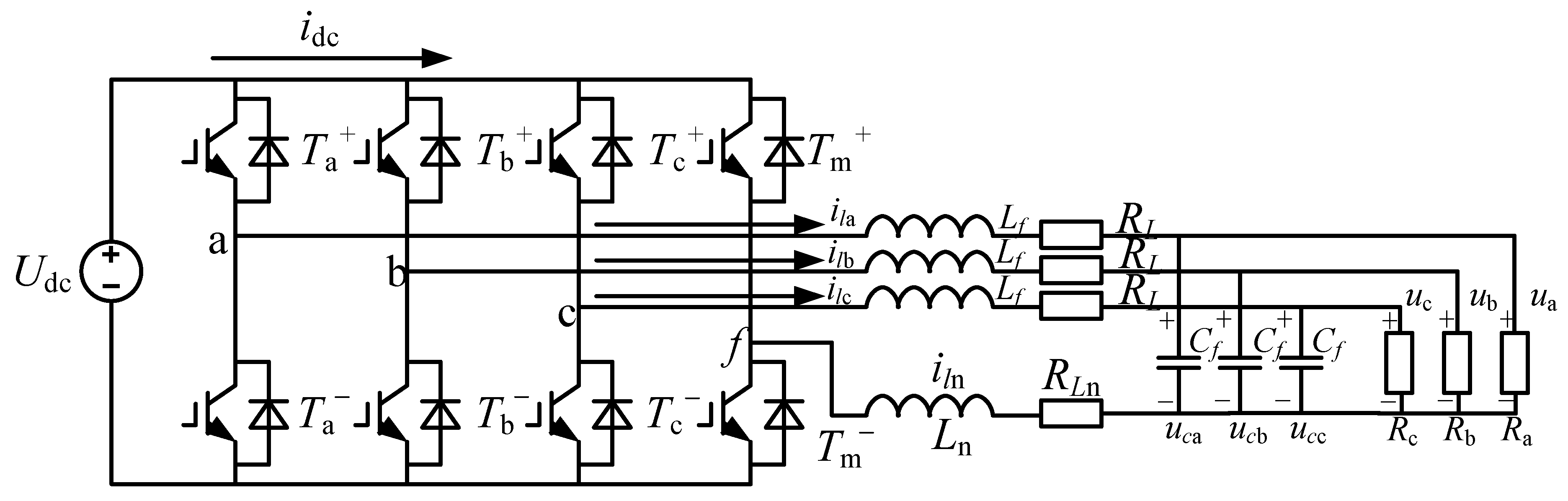
Figure 1 shows the equivalent circuit of the 3P4L converter. The fourth leg is added based on the traditional three-phase three-leg converter, and the midpoint of this leg is connected to the neutral point of the load through an inductor, L_n. In the figure, i_la, i_lb, i_lc, and i_ln represent the phase currents flowing into the filter inductors of phases a, b, c, and the fourth leg, respectively. u_ca, u_cb and u_cc are the capacitor voltages of the filtering capacitors in phases a, b, and c, respectively. U_dc and i_dc denote the DC bus voltage and current. L_f and C_f are the filter inductor and filter capacitor of the converter output, respectively. R_L is the equivalent resistance of the filter inductor and the dead-time effect. L_n is the neutral inductor (assuming L_n = L_f). u_a, u_b, and u_c are the three-phase symmetric output converter voltages.

Since a large number of variables are introduced in Figure 1, the meanings of each variable are now summarized in

Table 1. List of variables.

Variable	Definition	Units	Role
Udc	The DC bus voltage.	V	This provides a stable DC power supply.
idc	The DC bus current.	A	This provides a stable DC.
ila, ilb, ilc	The filtering inductor currents flowing through the filtering inductors of phases a, b, and c.	A	When the current passing through an inductor changes, it stores magnetic field energy and releases the energy when the current decreases.
iln	The filtering inductor current flowing through the filtering inductor of the neutral line leg.	A	The neutral line current of a 3P4L converter provides a direct path for a zero-sequence current.
Ta, Tb, Tc	The switching functions of the power switching devices of the legs of phases a, b, and c.	/	The switching duty cycle plays important roles in regulating output voltage, balancing neutral point potential, controlling output current, and suppressing harmonics.
Tm	The switching function of the power switching device in the neutral line leg.	/	The duty cycle of the fourth leg is a key control variable for 3P4L converters to address load imbalance, suppress harmonics, and enhance reliability.
uca, ucb, ucc	The voltages of the filtering capacitors of phases a, b, and c.	V	Three-phase capacitors and inductors form an LC filter, which utilizes the low impedance of capacitors to high-frequency harmonics to absorb or bypass harmonic currents, suppress voltage waveform distortion, and reduce the total harmonic distortion.
ua, ub, uc	The voltages of the loads of phases a, b, and c.	V	The load voltage is not only a carrier for energy transmission but also a core guarantee for the stable, efficient and reliable operation of the system.
Lf	The filter inductor.	H	The filtering inductor can utilize its characteristic of impeding current changes to suppress sudden current changes, limit the amplitude and rising rate of overcurrents, and provide protection for the converter and the load.
Cf	The filter capacitor.	F	Based on the fact that the filtering inductor impedes the change in the current, the filtering capacitor can further stabilize the output voltage.
Ln	The filtering inductor of the neutral line leg.	H	Since the neutral line inductor can suppress the propagation of abnormal currents such as the zero-sequence current, it reduces current fluctuations and distortion. This helps to reduce the intensity of electromagnetic interference.
RL	The series equivalent resistance of the filter capacitor.	Ω	Unlike an ideal inductor, the series equivalent resistance in an actual inductor does impede the current. When the inductor is connected to a circuit, especially at the moment of powering on, the current does not rise rapidly without limit as in an ideal inductor. Instead, it is restricted by the series equivalent resistance and rises gradually according to a specific rule. This can play a role in preventing excessive sudden changes in the current and protecting circuit components in some circuits.

.

Figure 1 shows the equivalent circuit of the 3P4L converter. The fourth leg is added based on the traditional three-phase three-leg converter, and the midpoint of this leg is connected to the neutral point of the load through an inductor, L_n. In the figure, i_la, i_lb, i_lc, and i_ln represent the phase currents flowing into the filter inductors of phases a, b, c, and the fourth leg, respectively. u_ca, u_cb and u_cc are the capacitor voltages of the filtering capacitors in phases a, b, and c, respectively. U_dc and i_dc denote the DC bus voltage and current. L_f and C_f are the filter inductor and filter capacitor of the converter output, respectively. R_L is the equivalent resistance of the filter inductor and the dead-time effect. L_n is the neutral inductor (assuming L_n = L_f). u_a, u_b, and u_c are the three-phase symmetric output converter voltages. T_i (i = a, b, c, m) represents the switching functions of the switching tubes on each leg.

$$\left\{\begin{array}{l}{T}_{\mathrm{am}}=T_{\mathrm{a}}-T_{\mathrm{m}}\\ T_{\mathrm{bm}}=T_{\mathrm{b}}-T_{\mathrm{m}}\hspace{1em}\\ T_{\mathrm{cm}}=T_{\mathrm{c}}-T_{\mathrm{m}}\end{array}\right.$$

(1)

By performing the switching cycle average operation and filtering out the switching frequency harmonic components, the phase duty cycles d_am, d_bm, and d_cm are obtained. Analyzing the current loop, the following can be derived:

$$\begin{array}{c}{i}_{\mathrm{dc}}=d_{\mathrm{a}}{i}_{l\mathrm{a}}+d_{\mathrm{b}}{i}_{l\mathrm{b}}+d_{\mathrm{c}}{i}_{l\mathrm{c}}+d_{\mathrm{m}}{i}_{l\mathrm{n}}\\ =d_{\mathrm{am}}{i}_{l\mathrm{a}}+d_{\mathrm{bm}}{i}_{l\mathrm{b}}+d_{\mathrm{cm}}{i}_{l\mathrm{c}}\end{array}$$

(2)

where d_a, d_b, and d_c are the duty cycles of phases a, b and c, respectively. d_m is the duty cycle of the fourth neutral line arm.

$$U_{\mathrm{dc}}\left[\begin{array}{c}{d}_{\mathrm{am}}\\ d_{\mathrm{bm}}\\ d_{\mathrm{cm}}\end{array}\right]=L_f\left[\begin{array}{c}{\displaystyle \frac{\mathrm{d}{i}_{l\mathrm{a}}}{\mathrm{d}t}}\\ {\displaystyle \frac{\mathrm{d}{i}_{l\mathrm{b}}}{\mathrm{d}t}}\\ {\displaystyle \frac{\mathrm{d}{i}_{l\mathrm{c}}}{\mathrm{d}t}}\end{array}\right]+R\left[\begin{array}{c}{i}_{l\mathrm{a}}\\ i_{l\mathrm{b}}\\ i_{l\mathrm{c}}\end{array}\right]+\left[\begin{array}{c}{u}_{c\mathrm{a}}\\ u_{c\mathrm{b}}\\ u_{c\mathrm{c}}\end{array}\right]-L_{\mathrm{n}}{\displaystyle \frac{\mathrm{d}{i}_{l\mathrm{n}}}{\mathrm{d}t}}-R{i}_{l\mathrm{n}}$$

(3)

$$U_{\mathrm{dc}}\left[\begin{array}{c}{d}_{\mathrm{am}}\\ d_{\mathrm{bm}}\\ d_{\mathrm{cm}}\end{array}\right]=L_f\left[\begin{array}{ccc}2& 1& 1\\ 1& 2& 1\\ 1& 1& 2\end{array}\right]\left[\begin{array}{c}{\displaystyle \frac{\mathrm{d}{i}_{l\mathrm{a}}}{\mathrm{d}t}}\\ {\displaystyle \frac{\mathrm{d}{i}_{l\mathrm{b}}}{\mathrm{d}t}}\\ {\displaystyle \frac{\mathrm{d}{i}_{l\mathrm{c}}}{\mathrm{d}t}}\end{array}\right]+R\left[\begin{array}{ccc}2& 1& 1\\ 1& 2& 1\\ 1& 1& 2\end{array}\right]\left[\begin{array}{c}{i}_{l\mathrm{a}}\\ i_{l\mathrm{b}}\\ i_{l\mathrm{c}}\end{array}\right]+\left[\begin{array}{c}{u}_{c\mathrm{a}}\\ u_{c\mathrm{b}}\\ u_{c\mathrm{c}}\end{array}\right]$$

(4)

From Equation (4), it can be seen that due to the influence of the neutral inductor, the system’s legs are mutually coupled and cannot be simply treated as three independent converter systems. Therefore, decoupling the control of the 3P4L converter is difficult to achieve in the three-phase stationary coordinate system.

Similarly, the capacitor voltages of the 3P4L converter can be expressed as follows:

$$C_f\left[\begin{array}{c}{\displaystyle \frac{\mathrm{d}{u}_{c\mathrm{a}}}{\mathrm{d}t}}\\ {\displaystyle \frac{\mathrm{d}{u}_{c\mathrm{b}}}{\mathrm{d}t}}\\ {\displaystyle \frac{\mathrm{d}{u}_{c\mathrm{c}}}{\mathrm{d}t}}\end{array}\right]=\left[\begin{array}{c}{i}_{l\mathrm{a}}\\ i_{l\mathrm{b}}\\ i_{l\mathrm{c}}\end{array}\right]-\left[\begin{array}{c}{i}_{\mathrm{am}}\\ i_{\mathrm{bm}}\\ i_{\mathrm{cm}}\end{array}\right]$$

(5)

where u_ca, u_cb and u_cc denote the capacitor voltages of the filtering capacitors in phases a, b, and c, respectively. i_am, i_bm and i_cm represent the modulated output currents of the three phases. Through the algebraic manipulation of the circuit equations, the following relationship is derived:

$$\left[\begin{array}{c}{\displaystyle \frac{\mathrm{d}{u}_{c\mathrm{a}}}{\mathrm{d}t}}\\ {\displaystyle \frac{\mathrm{d}{u}_{c\mathrm{b}}}{\mathrm{d}t}}\\ {\displaystyle \frac{\mathrm{d}{u}_{c\mathrm{c}}}{\mathrm{d}t}}\end{array}\right]={\displaystyle \frac{1}{C_f}}\left[\begin{array}{c}{i}_{l\mathrm{a}}\\ i_{l\mathrm{b}}\\ i_{l\mathrm{c}}\end{array}\right]-{\displaystyle \frac{1}{R{C}_f}}\left[\begin{array}{c}{u}_{\mathrm{a}}\\ u_{\mathrm{b}}\\ u_{\mathrm{c}}\end{array}\right].$$

(6)

2.2. The Formulation of the System Model in the Rotating Reference Frame

As can be seen from the analysis in the previous section, since the coupling terms contain differential elements, it is rather troublesome to implement the control. To fully decouple the model and make it easier to implement the control, the three-phase stationary coordinate system can be transformed into a coordinate system that rotates synchronously at the fundamental frequency of the converter power supply through coordinate transformation. After the transformation, the d-axis and q-axis controllers can be fully decoupled, and the fundamental sinusoidal quantities in the stationary coordinate system are transformed into DC quantities, which is beneficial for the design of the controller.

The transformation matrix for the transformation from the stationary coordinate system (a, b, and c) to the rotating coordinate system (d, q, and 0) is as follows:

$$T_{\mathrm{abc}/dqo}={\displaystyle \frac{2}{3}}\left[\begin{array}{ccc}\cos (\omega t)& \cos (\omega t-{\displaystyle \frac{2\pi }{3}})& \cos (\omega t+{\displaystyle \frac{2\pi }{3}})\\ \sin (\omega t)& \sin (\omega t-{\displaystyle \frac{2\pi }{3}})& \sin (\omega t+{\displaystyle \frac{2\pi }{3}})\\ {\displaystyle \frac{1}{2}}& {\displaystyle \frac{1}{2}}& {\displaystyle \frac{1}{2}}\end{array}\right].$$

(7)

After the transformation of the system model, the following expression can be obtained:

$${\displaystyle \frac{\mathrm{d}}{\mathrm{d}t}}\left[\begin{array}{c}{i}_d\\ i_q\\ i_0\end{array}\right]=\left[\begin{array}{ccc}0& -\omega & 0\\ \omega & 0& 0\\ 0& 0& 0\end{array}\right]\left[\begin{array}{c}{i}_d\\ i_q\\ i_0\end{array}\right]+{\displaystyle \frac{U_{\mathrm{dc}}}{L_f}}\left[\begin{array}{c}{d}_d\\ d_q\\ d_0\end{array}\right]-{\displaystyle \frac{R}{L_f}}\left[\begin{array}{c}{i}_d\\ i_q\\ i_0\end{array}\right]-{\displaystyle \frac{1}{L_f}}\left[\begin{array}{c}{U}_d\\ U_q\\ U_0\end{array}\right]-3{\displaystyle \frac{\mathrm{d}}{\mathrm{d}t}}\left[\begin{array}{c}0\\ 0\\ i_0\end{array}\right]-{\displaystyle \frac{3R}{L_f}}\left[\begin{array}{c}0\\ 0\\ i_0\end{array}\right],$$

(8)

$${\displaystyle \frac{\mathrm{d}}{\mathrm{d}t}}\left[\begin{array}{c}{U}_d\\ U_q\\ U_0\end{array}\right]={\displaystyle \frac{1}{C_f}}\left[\begin{array}{c}{i}_d\\ i_q\\ i_0\end{array}\right]+\left[\begin{array}{ccc}0& -\omega & 0\\ \omega & 0& 0\\ 0& 0& 0\end{array}\right]\left[\begin{array}{c}{U}_d\\ U_q\\ U_0\end{array}\right],$$

(9)

where i_d, i_q and i₀ are the direct-axis current, the quadrature-axis current, and the zero-sequence current, respectively. U_d, U_q and U₀ are the direct-axis voltage, the quadrature-axis voltage, and the zero-sequence voltage, respectively.

That is,

$${\displaystyle \frac{\mathrm{d}}{\mathrm{d}t}}\left[\begin{array}{c}{i}_d\\ i_q\\ 4i_0\end{array}\right]=\left[\begin{array}{ccc}-{\displaystyle \frac{R}{L_f}}& -\omega & 0\\ \omega & -{\displaystyle \frac{R}{L_f}}& 0\\ 0& 0& -{\displaystyle \frac{4R}{L_f}}\end{array}\right]\left[\begin{array}{c}{i}_d\\ i_q\\ i_0\end{array}\right]+{\displaystyle \frac{U_{\mathrm{dc}}}{L_f}}\left[\begin{array}{c}{d}_d\\ d_q\\ d_0\end{array}\right]-{\displaystyle \frac{1}{L_f}}\left[\begin{array}{c}{U}_d\\ U_q\\ U_0\end{array}\right].$$

(10)

2.3. Discretization of Equivalent Mathematical Model for 3P4L Converter in Stationary Coordinate System

The mathematical model of the 3P4L converter can be discretized using the RK4 method. This method is a commonly used numerical solution for ordinary differential equations, offering advantages such as high precision, good stability, high versatility, and simple implementation. Without posing significant computational challenges, it provides high computational accuracy [17]. For the modeling of the 3P4L converter, the error can be considered negligible.

The state-space model of three-phase inductor currents (i_la, i_lb, and i_lc) and capacitor voltages (u_ca, u_cb, and u_cc) for 3P4L converters is reformulated as follows:

$$\left\{\begin{array}{l}h(i_{l\mathrm{a}})={\displaystyle \frac{\mathrm{d}{i}_{l\mathrm{a}}}{\mathrm{d}t}}\\ h(i_{l\mathrm{b}})={\displaystyle \frac{\mathrm{d}{i}_{l\mathrm{b}}}{\mathrm{d}t}}\\ h(i_{l\mathrm{c}})={\displaystyle \frac{\mathrm{d}{i}_{l\mathrm{c}}}{\mathrm{d}t}}\end{array}\right.; \left\{\begin{array}{l}p(u_{c\mathrm{a}})={\displaystyle \frac{\mathrm{d}{u}_{c\mathrm{a}}}{\mathrm{d}t}}\\ p(u_{c\mathrm{b}})={\displaystyle \frac{\mathrm{d}{u}_{c\mathrm{b}}}{\mathrm{d}t}}\\ p(u_{c\mathrm{c}})={\displaystyle \frac{\mathrm{d}{u}_{c\mathrm{c}}}{\mathrm{d}t}}\end{array}\right..$$

(11)

In the stationary coordinate system, the RK4 discretization expressions for three-phase inductor currents and capacitor voltages of the 3P4L converter are formulated as follows:

$$\left\{\begin{array}{l}{i}_{l\mathrm{a},n+1}=i_{l\mathrm{a},n}+{\displaystyle \frac{h}{6}}(k_{e1}+2k_{e2}+2k_{e3}+k_{e4})\\ i_{l\mathrm{b},n+1}=i_{l\mathrm{b},n}+{\displaystyle \frac{h}{6}}(k_{f1}+2k_{f2}+2k_{f3}+k_{f4})\\ i_{l\mathrm{c},n+1}=i_{l\mathrm{c},n}+{\displaystyle \frac{h}{6}}(k_{g1}+2k_{g2}+2k_{g3}+k_{g4})\end{array}\right.$$

(12)

$$\left\{\begin{array}{l}{u}_{c\mathrm{a},n+1}=u_{c\mathrm{a},n}+{\displaystyle \frac{h}{6}}(k_{r1}+2k_{r2}+2k_{r3}+k_{r4})\\ u_{c\mathrm{b},n+1}=u_{c\mathrm{b},n}+{\displaystyle \frac{h}{6}}(k_{j1}+2k_{j2}+2k_{j3}+k_{j4})\\ u_{c\mathrm{c},n+1}=u_{c\mathrm{c},n}+{\displaystyle \frac{h}{6}}(k_{k1}+2k_{k2}+2k_{k3}+k_{k4})\end{array}\right.$$

(13)

where h represents the computational step time between the n-th and (n + 1)-th time steps. i_lk,n+1 (with k = a, b, c) is the value of the inductor current at the (n + 1)-th node. The calculation method for u_ck,n+1 is the same as that for the inductor current. Since the inductor current and the capacitor voltage are coupled with each other in the natural coordinate system, the three phases a, b and c need to be represented separately. k_i1–k_i4 (i = e, f, r, j) are used to calculate the average rate of change between the n-th and (n + 1)-th steps, which are expressed as follows:

$$\left\{\begin{array}{l}{k}_{e1}=f_1(x_n,y_n)\\ k_{r1}=f_2(x_n,y_n)\\ k_{e2}=f_1(x_n+{\displaystyle \frac{h}{2}}{k}_{e1},y_n+{\displaystyle \frac{h}{2}}{k}_{r1})\\ k_{r2}=f_2(x_n+{\displaystyle \frac{h}{2}}{k}_{e1},y_n+{\displaystyle \frac{h}{2}}{k}_{r1})\\ k_{e3}=f_1(x_n+{\displaystyle \frac{h}{2}}{k}_{e2},y_n+{\displaystyle \frac{h}{2}}{k}_{r2})\\ k_{r3}=f_2(x_n+{\displaystyle \frac{h}{2}}{k}_{e2},y_n+{\displaystyle \frac{h}{2}}{k}_{r2})\\ k_{e4}=f_1(x_n+h{k}_{e3},y_n+h{k}_{r3})\\ k_{r4}=f_2(x_n+h{k}_{e3},y_n+h{k}_{r3})\end{array}\right.$$

(14)

$$\left\{\begin{array}{l}{k}_{f1}=f_1(x_n,y_n)\\ k_{j1}=f_2(x_n,y_n)\\ k_{f2}=f_1(x_n+{\displaystyle \frac{h}{2}}{k}_{f1},y_n+{\displaystyle \frac{h}{2}}{k}_{j1})\\ k_{j2}=f_2(x_n+{\displaystyle \frac{h}{2}}{k}_{f1},y_n+{\displaystyle \frac{h}{2}}{k}_{j1})\\ k_{f3}=f_1(x_n+{\displaystyle \frac{h}{2}}{k}_{f2},y_n+{\displaystyle \frac{h}{2}}{k}_{j2})\\ k_{j3}=f_2(x_n+{\displaystyle \frac{h}{2}}{k}_{f2},y_n+{\displaystyle \frac{h}{2}}{k}_{j2})\\ k_{f4}=f_1(x_n+h{k}_{f3},y_n+h{k}_{j3})\\ k_{j4}=f_2(x_n+h{k}_{f3},y_n+h{k}_{j3})\end{array}\right..$$

(15)

2.4. Control Implementation

As can be seen from Equation (9), when controlling in the three-phase rotating coordinate system, the fourth leg is fully decoupled from the other legs. As can be seen from Figure 2, when converting the 3P4L converter into a three-channel signal model of d, q, and 0, there are coupling terms between the d and q channels: −ωC_fU_q, ωC_fU_d, −ωL_fi_q, ωL_fi_d. The inductor currents of the d-axis and q-axis are coupled to the q-axis and d-axis, respectively, in the form of controlled voltage sources, while the output voltages of the d-axis and q-axis are coupled to the q-axis and d-axis in the form of controlled current sources. The 0 channel is completely independent of the other two channels and only contains zero-sequence components, which can be independently controlled from the positive and negative sequence components.

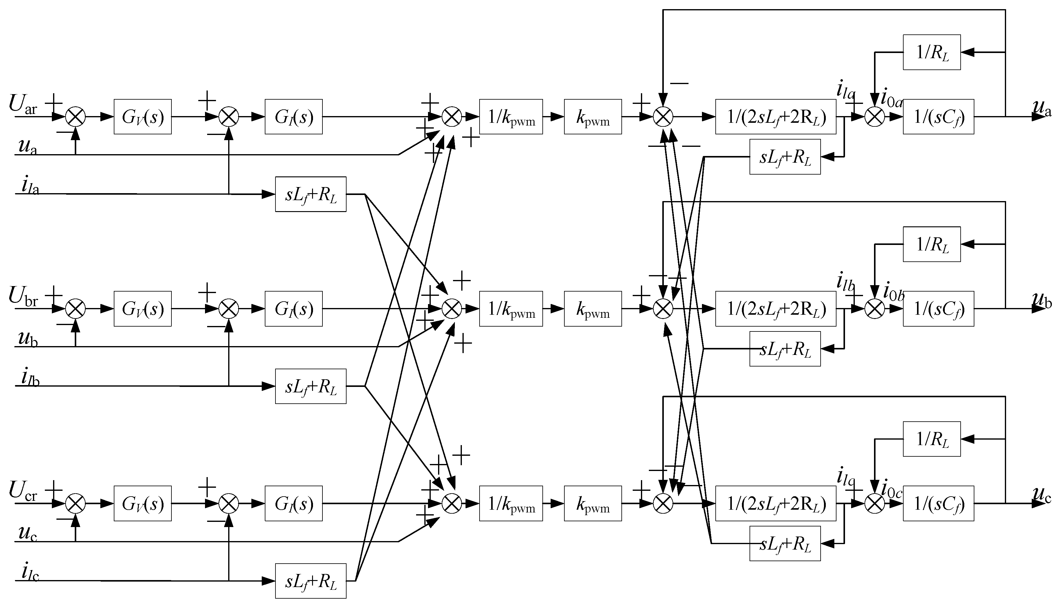
Therefore, appropriate control terms need to be added to eliminate the coupling relationship between the d and q axes. As shown in Figure 3, system decoupling can thereby be achieved, and the decoupled 3P4L converter can be equivalently treated as three single-phase converters for independent control.

2.5. Mathematical Model of Controller for 3p4l Converters

The complete implementation process of the control system for a 3P4L converter can be expressed as follows:

As shown in Figure 4, the dual closed-loop control of PI voltage and current is employed to conduct closed-loop regulation for the 3P4L converter.

The mathematical expression for the current inner loop of the 3P4L converter controller is as follows:

$$\left\{\begin{array}{l}{i}_{d,\mathrm{e}}=i_{d,\mathrm{ref}}-i_{\mathrm{o}\_d}\\ i_{q,\mathrm{e}}=i_{q,\mathrm{ref}}-i_{\mathrm{o}\_q}\\ i_{0,\mathrm{e}}=i_{0,\mathrm{ref}}-i_{\mathrm{o}\_0}\\ u_{d,\mathrm{m}}=k_{\mathrm{p}}{i}_{d,\mathrm{e}}(t)+k_{\mathrm{i}}{\displaystyle {\int }_0^t{i}_{d,\mathrm{e}}(t)\mathrm{d}t}\\ u_{q,\mathrm{m}}=k_{\mathrm{p}}{i}_{q,\mathrm{e}}(t)+k_{\mathrm{i}}{\displaystyle {\int }_0^t{i}_{q,\mathrm{e}}(t)\mathrm{d}t}\\ u_{0,\mathrm{m}}=k_{\mathrm{p}}{i}_{0,\mathrm{e}}(t)+k_{\mathrm{i}}{\displaystyle {\int }_0^t{i}_{0,\mathrm{e}}(t)\mathrm{d}t}\end{array}\right.$$

(16)

where i_d,e, i_q,e and i_0,e are the differences between the reference values of the current inner loop on the d–axis, q–axis and 0–axis in the rotating coordinate system. i_{o_d}, i_{o_q} and i_{o_0} are the three-phase inductor currents in the rotating coordinate system, and u_d,m, u_q,m and u_0,m are the output signals of the PI controller.

The output values of the PI controller in the outer voltage loop of the 3P4L converter are used as the reference values of the current for the inner loop control. The mathematical expression of the outer voltage loop of the 3P4L converter controller is as follows:

$$\left\{\begin{array}{l}{u}_{d,\mathrm{e}}=u_{d,\mathrm{ref}}-u_{\mathrm{o}\_d}\\ u_{q,\mathrm{e}}=u_{q,\mathrm{ref}}-u_{\mathrm{o}\_q}\\ u_{0,\mathrm{e}}=u_{0,\mathrm{ref}}-u_{\mathrm{o}\_0}\\ i_{d,\mathrm{ref}}=k_{\mathrm{p}}{u}_{d,\mathrm{e}}(t)+k_{\mathrm{i}}{\displaystyle {\int }_0^t{u}_{d,\mathrm{e}}(t)\mathrm{d}t}\\ i_{q,\mathrm{ref}}=k_{\mathrm{p}}{u}_{q,\mathrm{e}}(t)+k_{\mathrm{i}}{\displaystyle {\int }_0^t{u}_{q,\mathrm{e}}(t)\mathrm{d}t}\\ i_{0,\mathrm{ref}}=k{u}_{0,\mathrm{e}}(t)+k_{\mathrm{i}}{\displaystyle {\int }_0^t{u}_{0,\mathrm{e}}(t)\mathrm{d}t}\end{array}\right.$$

(17)

where u_d,ref is the d–axis reference voltage of the 3P4L converter, which is usually set as the amplitude of the rated voltage. u_q,ref is the q–axis reference voltage of the 3P4L converter, which is typically set to 0. u_0,ref is the 0-axis reference voltage of the 3P4L converter, and its reference value is generally set as the opposite of the algebraic sum of the currents of the a, b, and c phase legs. u_d,e, u_q,e and u_0,e are the differences between the reference values of the outer voltage loop on the d-axis, q-axis, and 0-axis in the rotating coordinate system and the three-phase capacitor voltages, respectively. i_d,ref, i_q,ref and i_0,ref are the output signals of the outer voltage loop of the PI controller, which also serve as the reference values for the inner current loop.

The discrete model of the closed-loop controller for the inner current loop is

$$\left\{\begin{array}{l}{i}_{d,\mathrm{e},\mathrm{n}}=i_{d,\mathrm{e},\mathrm{n}+1}\\ i_{q,\mathrm{e},\mathrm{n}}=i_{q,\mathrm{e},\mathrm{n}+1}\\ i_{0,\mathrm{e},\mathrm{n}}=i_{0,\mathrm{e},\mathrm{n}+1}\\ u_{d,\mathrm{m},\mathrm{n}}=u_{d,\mathrm{m},\mathrm{n}+1}\\ u_{q,\mathrm{m},\mathrm{n}}=u_{q,\mathrm{m},\mathrm{n}+1}\\ u_{0,\mathrm{m},\mathrm{n}}=u_{0,\mathrm{m},\mathrm{n}+1}\\ i_{d,\mathrm{e},\mathrm{n}+1}=i_{d,\mathrm{ref}}-i_{\mathrm{o}\_d,\mathrm{n}+1}\\ i_{q,\mathrm{e},\mathrm{n}+1}=i_{q,\mathrm{ref}}-i_{\mathrm{o}\_q,\mathrm{n}+1}\\ i_{0,\mathrm{e},\mathrm{n}+1}=i_{0,\mathrm{ref}}-i_{\mathrm{o}\_0,\mathrm{n}+1}\\ u_{d,\mathrm{m},\mathrm{n}+1}=u_{d,\mathrm{m},\mathrm{n}}+k_{\mathrm{p}}(i_{d,\mathrm{e},\mathrm{n}+1}-i_{d,\mathrm{e},\mathrm{n}})+k_{\mathrm{i}}h{i}_{d,\mathrm{e},\mathrm{n}+1}\\ u_{q,\mathrm{m},\mathrm{n}+1}=u_{q,\mathrm{m},\mathrm{n}}+k_{\mathrm{p}}(i_{q,\mathrm{e},\mathrm{n}+1}-i_{q,\mathrm{e},\mathrm{n}})+k_{\mathrm{i}}h{i}_{q,\mathrm{e},\mathrm{n}+1}\\ u_{0,\mathrm{m},\mathrm{n}+1}=u_{0,\mathrm{m},\mathrm{n}}+k_{\mathrm{p}}(i_{0,\mathrm{e},\mathrm{n}+1}-i_{0,\mathrm{e},\mathrm{n}})+k_{\mathrm{i}}h{i}_{0,\mathrm{e},\mathrm{n}+1}\end{array}\right..$$

(18)

The discrete model of the closed-loop controller for the outer voltage loop is

$$\left\{\begin{array}{l}{u}_{d,\mathrm{e},\mathrm{n}}=u_{d,\mathrm{e},\mathrm{n}+1}\\ u_{q,\mathrm{e},\mathrm{n}}=u_{q,\mathrm{e},\mathrm{n}+1}\\ u_{0,\mathrm{e},\mathrm{n}}=u_{0,\mathrm{e},\mathrm{n}+1}\\ i_{d,\mathrm{ref},\mathrm{n}}=i_{d,\mathrm{ref},\mathrm{n}+1}\\ i_{q,\mathrm{ref},\mathrm{n}}=i_{q,\mathrm{ref},\mathrm{n}+1}\\ i_{0,\mathrm{ref},\mathrm{n}}=i_{0,\mathrm{ref},\mathrm{n}+1}\\ u_{d,\mathrm{e},\mathrm{n}+1}=u_{d,\mathrm{ref}}-u_{\mathrm{o}\_d,\mathrm{n}+1}\\ u_{q,\mathrm{e},\mathrm{n}+1}=u_{q,\mathrm{ref}}-u_{\mathrm{o}\_q,\mathrm{n}+1}\\ u_{0,\mathrm{e},\mathrm{n}+1}=u_{0,\mathrm{ref}}-u_{\mathrm{o}\_0,\mathrm{n}+1}\\ i_{d,\mathrm{ref},\mathrm{n}+1}=i_{d,\mathrm{m},\mathrm{n}}+k_{\mathrm{p}}(u_{d,\mathrm{e},\mathrm{n}+1}-u_{d,\mathrm{e},\mathrm{n}})+k_{\mathrm{i}}h{u}_{d,\mathrm{e},\mathrm{n}+1}\\ i_{q,\mathrm{ref},\mathrm{n}+1}=i_{q,\mathrm{m},\mathrm{n}}+k_{\mathrm{p}}(u_{q,\mathrm{e},\mathrm{n}+1}-u_{q,\mathrm{e},\mathrm{n}})+k_{\mathrm{i}}h{u}_{q,\mathrm{e},\mathrm{n}+1}\\ i_{0,\mathrm{ref},\mathrm{n}+1}=i_{0,\mathrm{m},\mathrm{n}}+k_{\mathrm{p}}(u_{0,\mathrm{e},\mathrm{n}+1}-u_{0,\mathrm{e},\mathrm{n}})+k_{\mathrm{i}}h{u}_{0,\mathrm{e},\mathrm{n}+1}\end{array}\right..$$

(19)

2.6. The Three-Dimensional Space Vector Modulation of 3P4L Converters in the Stationary Coordinate System

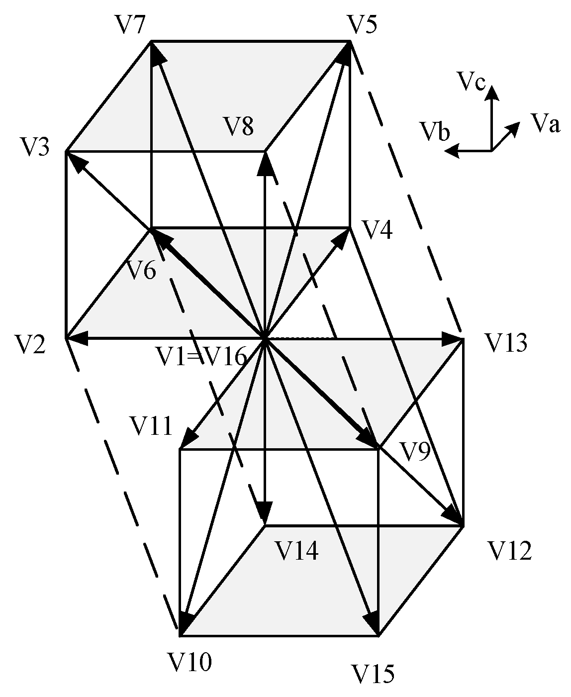
A 3P4L converter has four legs, each with two switching states as shown in Equation (20), resulting in a total of 2⁴ = 16 switching vectors for the four legs of the 3P4L converter.

$$S_i=\left\{\begin{array}{c}1 \begin{array}{c}(\mathrm{upper} \mathrm{switch} \mathrm{is} \mathrm{turned} \mathrm{on}, \mathrm{lower} \mathrm{switch} \mathrm{is} \mathrm{turned} \mathrm{off})\end{array}\\ 0 \begin{array}{c}(\mathrm{upper} \mathrm{switch} \mathrm{is} \mathrm{turned} \mathrm{off}, \mathrm{lower} \mathrm{switch} \mathrm{is} \mathrm{turned} \mathrm{on})\end{array}\end{array}\right.$$

(20)

The sixteen voltage vectors in the stationary coordinate system are shown in

Table 2. Output voltage vectors in the stationary coordinate system.

Serial Number	a	b	c	m	Vam	Vbm	Vcm	Synthetic Vector
1	0	0	0	0	0	0	0	V1
2	0	0	1	0	0	0	1	V2
3	0	1	0	0	0	1	0	V3
4	0	1	1	0	0	1	1	V4
5	1	0	0	0	1	0	0	V5
6	1	0	1	0	1	0	1	V6
7	1	1	0	0	1	1	0	V7
8	1	1	1	0	1	1	1	V8
9	0	0	0	1	−1	−1	−1	V9
10	0	0	1	1	−1	−1	0	V10
11	0	1	0	1	−1	0	−1	V11
12	0	1	1	1	−1	0	0	V12
13	1	0	0	1	0	−1	−1	V13
14	1	0	1	1	0	−1	0	V14
15	1	1	0	1	0	0	−1	V15
16	1	1	1	1	0	0	0	V16

.

Among them, V1 and V16 are zero vectors, and the remaining 14 are non-zero switching vectors.

As shown in Figure 5, in the stationary coordinate system, the 16 switching vectors are mapped to a closed dodecahedron structure composed of two cubes with a side length of 1. This dodecahedron is divided into 24 tetrahedrons. As long as it is determined which specific tetrahedron among the 24 tetrahedrons the reference voltage vector is located in, adjacent non-zero vectors and zero vectors can be selected for synthesis. Then, through calculation, the action time of each vector can be obtained. Finally, by combining them in a certain order, the 3D-SVPWM modulation strategy in the stationary coordinate system can be realized.

We define the parameters k₁-k₆ as follows:

$$k_1=\left\{\begin{array}{c}1\left(u_{{\mathrm{a}}_{-}\mathrm{ef}}\ge 0\right)\\ 0\left(u_{{\mathrm{a}}_{-}\mathrm{ef}}<0\right)\end{array}\right. k_4=\left\{\begin{array}{c}1\left(u_{{\mathrm{a}}_{-}\mathrm{ef}}-u_{{\mathrm{b}}_{-}\mathrm{ef}}\ge 0\right)\\ 0\left(u_{{\mathrm{a}}_{-}\mathrm{ef}}-u_{{\mathrm{b}}_{-}\mathrm{ef}}<0\right)\end{array}\right.$$

(21)

$$k_2=\left\{\begin{array}{c}1\left(u_{{\mathrm{b}}_{-}\mathrm{ef}}\ge 0\right)\\ 0\left(u_{{\mathrm{b}}_{-}\mathrm{ef}}<0\right)\end{array}\right. k_5=\left\{\begin{array}{c}1\left(u_{{\mathrm{b}}_{-}\mathrm{ef}}-u_{{\mathrm{c}}_{-}\mathrm{ef}}\ge 0\right)\\ 0\left(u_{{\mathrm{b}}_{-}\mathrm{ef}}-u_{{\mathrm{c}}_{-}\mathrm{ef}}<0\right)\end{array}\right.$$

(22)

$$k_3=\left\{\begin{array}{c}1\left(u_{{\mathrm{c}}_{-}\mathrm{ef}}\ge 0\right)\\ 0\left(u_{{\mathrm{c}}_{-}\mathrm{ef}}<0\right)\end{array}\right. k_6=\left\{\begin{array}{c}1\left(u_{{\mathrm{a}}_{-}\mathrm{ef}}-u_{{\mathrm{c}}_{-}\mathrm{ef}}\ge 0\right)\\ 0\left(u_{{\mathrm{a}}_{-}\mathrm{ef}}-u_{{\mathrm{b}}_{-}\mathrm{ef}}<0\right)\end{array}\right.$$

(23)

where u_{a_ref}, u_{b_ref}, and u_{c_ref} are given voltage reference vectors, and k₁-k₆ have values of 1 or 0.

We define the pointer function as follows:

$$\mathrm{RP}=1+{\displaystyle \sum _{i=1}^6{k}_i}·2^{(\mathrm{i}-1)}.$$

(24)

By substituting the calculated k values into the pointer function RP, it can be concluded that there are a total of 24 values of RP, and each value of RP corresponds to 1 of the 24 tetrahedra. After calculation, the corresponding relationship between RP and voltage vectors is shown in

Table 3. The one-to-one correspondence between different values of RP and the corresponding non-zero switching vectors.

RP	d1	d2	d3	RP	d1	d2	d3
1	V9	V10	V12	41	V9	V13	V14
5	V2	V10	V12	42	V5	V13	V14
7	V2	V4	V12	46	V5	V6	V14
8	V2	V4	V8	48	V5	V6	V8
9	V9	V10	V14	49	V9	V11	V15
13	V2	V10	V14	51	V3	V11	V15
14	V2	V6	V14	52	V3	V7	V15
16	V2	V6	V8	56	V3	V7	V8
17	V9	V11	V12	57	V9	V13	V15
19	V3	V11	V12	58	V5	V13	V15
23	V3	V4	V12	60	V5	V7	V15
24	V3	V4	V12	64	V5	V7	V8

.

In summary, after the three non-zero switching vectors are determined, according to the principle of space vector synthesis, the corresponding duty cycles of the switching vectors can be calculated. The reference voltage vector V_ref can be calculated by the sum of the products of the switching vectors and their corresponding duty cycles. The calculation method of the duty cycles of the non-zero switching voltage vectors is as follows:

$$\left[\begin{array}{c}{d}_1\\ d_2\\ d_2\end{array}\right]={\left[\begin{array}{ccc}\mathrm{V}{d}_{1\mathrm{a}}& \mathrm{V}{d}_{2\mathrm{a}}& \mathrm{V}{d}_{3\mathrm{a}}\\ \mathrm{V}{d}_{1\mathrm{b}}& \mathrm{V}{d}_{2\mathrm{b}}& \mathrm{V}{d}_{3\mathrm{b}}\\ \mathrm{V}{d}_{1\mathrm{c}}& \mathrm{V}{d}_{2\mathrm{c}}& \mathrm{V}{d}_{3\mathrm{c}}\end{array}\right]}^{-1}\left[\begin{array}{c}{\mathrm{V}}_{\mathrm{am}}\\ {\mathrm{V}}_{\mathrm{bm}}\\ {\mathrm{V}}_{\mathrm{cm}}\end{array}\right]$$

(25)

where d₁, d₂ and d₃ are the duty cycles of the three non-zero switching voltage vectors, Vd1, Vd2 and Vd3 are the three non-zero switching voltage vectors, V_ref is the reference voltage vector, and the subscripts of Vd1, Vd2 and Vd3 are the projections of the non-zero switching voltage vectors in the stationary coordinate system. As long as the value of RP is determined, the action times of the non-zero vectors can be directly calculated through Equation (25).

3. Parameter Identification Method

The mathematical model of the 3P4L converter, as represented by Equation (26), is a highly nonlinear multi-variable function. Traditional solution methods (such as the Kalman filter and the least squares method) cannot be used to solve the model proposed in this paper. Therefore, the LF-WOA is employed to compute the converter model. The LF-WOA features a strong global search capability, good robustness and adaptability. It has a simple implementation process and shows good versatility for different models.

3.1. Objective Function

To achieve the real-time identification of the digital twin characteristic parameters of the 3P4L converter, the minimum sum of squared differences in the inductor current of the converter over a continuous time period is used as the objective function.

$$\min f_{\mathrm{obj}}={\displaystyle \frac{1}{N}}{\displaystyle \sum _{j=1}^N[{(i_{l\mathrm{a},j}-i_{l\mathrm{am},j})}^2}+{(i_{l\mathrm{b},j}-i_{l\mathrm{bm},j})}^2+{(i_{l\mathrm{c},j}-i_{l\mathrm{cm},j})}^2]$$

(26)

where i_la,j, i_lb,j, and i_lc,j are the inductor currents of phases a, b, and c of the digital twin of the 3P4L converter obtained through RK4 iterative calculation, respectively; i_lam,j, i_lbm,j, and i_lcm,j are the three-phase inductor currents output from the simulation or hardware-in-the-loop platform of the 3P4L converter; and N is the sample size of the measurement data.

The constraint is set to meet the critical threshold for the failure of the key components of the 3P4L converter.

$$\left\{\begin{array}{l}0.8L(t)\le L(t)\le 1.2L(t)\\ 0.8C(t)\le C(t)\le 1.2C(t)\\ 0<R_L(t)\le 2R_L(t)\end{array}\right.$$

(27)

In Equation (27), L(t), C(t), and R_L(t) are the actual values of the inductor, capacitor, and the equivalent series resistance of the inductor at time t, respectively.

3.2. Whale Optimization Algorithm

The WOA is a nature-inspired metaheuristic optimization algorithm proposed by Mirjalili and Lewis in 2016, which draws inspiration from the hunting behavior of humpback whales [18]. During hunting, humpback whales locate and encircle prey and then aggregate food into a bubble net using a spiral bubble net technique from the bottom up. Thus, in the prey-encircling phase of the WOA, the best search agent is considered the target prey or the position closest to the optimal solution. Other search agents strive to converge toward this best search agent, updating their positions through Equations (28)–(32).

$$X\left(t+1\right)=X^{*}\left(t\right)-A{D}^{\prime }$$

(28)

$$A=2a·\mathrm{rand}-a$$

(29)

$$D^{\prime }=|C{X}^{*}\left(t\right)-X\left(t\right)|$$

(30)

$$C=2\mathrm{rand}$$

(31)

$$a=2-{\displaystyle \frac{2t}{T_{\max }}}$$

(32)

In Equations (28)–(32), t is the current iteration number, A and C are coefficients, X represents the current solution position, and X* denotes the current optimal solution position. Parameter a decreases linearly from 2 to 0 during iterations, rand is a random number uniformly distributed in [0, 1], and T_max is the maximum number of iterations.

Mathematical modeling is conducted for the spiral bubble net, and optimization is performed. Random or the best search agents are used to simulate hunting behavior for prey pursuit, while the spiral is employed to mimic the bubble net attack mechanism of humpback whales.

$$X\left(t+1\right)=D^{\prime }{e}^{bl}\cos \left(2\pi l\right)+X^{*}\left(t\right)$$

(33)

$$D^{\prime }=\left|X^{*}\left(t\right)-X\left(t\right)\right|$$

(34)

In Equation (34), D′ denotes the distance between the ith individual and the optimal individual, b is a constant used to define the shape of the logarithmic spiral, and l is a random number between [−1, 1].

During the prey search stage, instead of choosing the current optimal individual as the target for position update, a whale randomly selects an individual from the current population as the target for position update. Therefore, the mathematical model for updating the position of whales in this stage is as follows:

$$D^{″}=|C{X}_{\mathrm{rand}}(t)-X(t)|$$

(35)

$$X(t+1)=X_{\mathrm{rand}}(t)-A{D}^{″}$$

(36)

where X_rand(t) is the position vector of a randomly selected whale individual and X(t) is the position vector of the current whale individual.

3.3. Levy Flight Strategy

The step size of a Levy flight is determined by u and v that follow a normal distribution. The flight strategy mainly involves short-distance searches and occasionally long-distance flights, which can effectively help individuals escape from local optima [19]. Whales with poor fitness update their positions using the Levy flight strategy. The step size of the Levy flight strategy is random, which enables both small-scale and large-scale searches. To some extent, this increases the population diversity of the algorithm and improves the optimization accuracy of the WOA.

In a Levy flight,

$$X_i^{t+1}=X_i^t+\mathrm{Levy}(\beta )\oplus \gamma .$$

(37)

In Equation (37), ⊕ denotes the dot product; γ is the step size control parameter; and Levy(β) represents the random search path.

Mantegna [20] proposed that the random step size s of the Levy Flight is represented by Equation (39):

$$\gamma =\mathrm{random}\left(\mathrm{size}\right(X_i\left)\right)$$

(38)

$$\mathrm{Levy}(\beta )~s={\displaystyle \frac{u}{{\left|v\right|}^{\frac{1}{\beta }}}}$$

(39)

$$u~N(0,{\sigma }_u^2),v~N(0,{\sigma }_v^2)$$

(40)

$${\sigma }_u^2={\left[{\displaystyle \frac{\Gamma (1+\beta )\sin (\pi \beta /2)}{\Gamma ((1+\beta )/2)\beta 2^{(\beta -1)/2}}}\right]}^{{\displaystyle \frac{1}{\beta }}},{\sigma }_v^2=1$$

(41)

where Γ(x) is the Gamma function. β ∈ (0,2).

3.4. Parameter Identification Method Based on LF-WOA

In summary, the LF-WOA is used to evaluate the characteristic parameters and their fitness of the 3P4L converter in real time. The specific process is as follows: First, sample a set of inductor current data of the digital twin of the 3P4L converter. With the critical conditions for the failure of the converter’s key components as constraints, preliminarily calculate the fitness value of the objective function f_obj. Then, according to the current number of iterations and randomly selected parameters, update the positions of the search agents according to the prey-encircling model or the bubble net attack model, so that the characteristic parameters of the established offline digital twin model gradually approach those of the actual system.

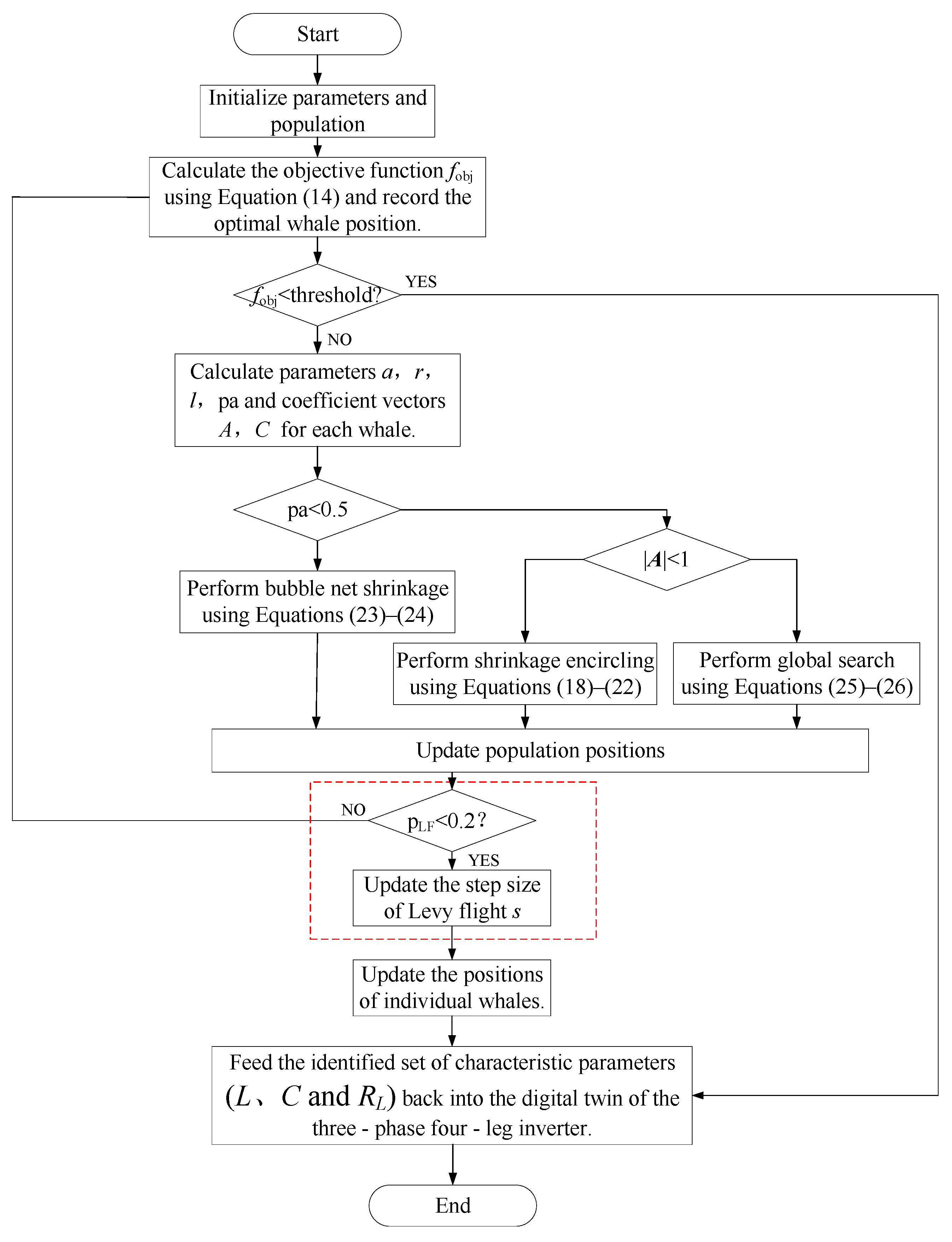
The flow chart of the LF-WOA for searching parameters is shown in Figure 6, and its steps are as follows:

(1)

Set the size of the whale population, the parameters of the Levy flight and the maximum number of iterations to initialize the whale position.

(2)

Preliminarily calculate the fitness value of the objective function f_obj using Equation (26).

(3)

If f_obj is less than the preset threshold 10⁻⁴, output the currently identified set of characteristic parameters. Otherwise, update parameter a according to Equation (32). Generate a random number for each whale position X(t), and calculate the coefficients A and C according to Equations (29) and (31).

(4)

Use random parameter p_a to determine the strategy for updating the whale positions. When p < 0.5, select the spiral position-updating mechanism. When p_a ≥ 0.5 and |A| ≥ 1, enter the prey-searching stage and update the whale positions using Equations (35) and (36). When |A| < 1, enter the prey-encircling stage and update the whale positions using Equations (28)–(32).

(5)

Determine whether the optimal whale individual will perform the Levy flight with a probability of 20%. If the conditions for the Levy flight are met, adjust the step size s of the Levy flight according to Equation (39), and update the whale’s position to the current position plus 0.1 s.

(6)

Check whether the updated whale position X(t + 1) is within the preset boundary conditions.

(7)

Input the updated whale position X(t + 1) into the digital twin model of the 3P4L converter to complete the closed loop.

(8)

When the number of iterations reaches T_max or the threshold is reached, output the global optimal position X* and the optimal fitness.

Figure 6. Block diagram of flow of LF-WOA search parameters.

Figure 6. Block diagram of flow of LF-WOA search parameters.

The specific parameters of the LF-WOA are shown in

Table 4. Specification of LF-WOA.

Specification	Value
Maximum number of iterations Tmax	35
Size of population N	20
Spiral shape parameter b	1
Dimensionality Dim	8
Levy flight parameters β	1.5

.

It should be noted that the step size distribution of the Levy flight is described by a stable distribution, and its probability density function satisfies the following:

$$f(x)~{\displaystyle \frac{1}{{\left|x\right|}^{1+\beta }}}$$

(42)

where Levy flight parameter β determines the tail characteristics of the distribution. When β is close to 2, the distribution approaches a normal distribution, and the variance of the step size is finite, corresponding to a strong local search ability. When β is close to 0, the variance of the step size is infinite, which means that extremely long step sizes occur occasionally, and the global search ability is strong. When the Levy flight strategy is adopted to improve the WOA, the value of β needs to balance the global exploration and local exploitation capabilities of the algorithm. The objective function of the LF-WOA in this paper is a complex multi-dimensional function. Therefore, β is set to 1.5, and a relatively large proportion of long-distance jumps are used to escape from local optima. In addition, reference [21] has proven that when there is no prior knowledge, in algorithms that imitate bird migration or insect foraging, setting β to 1.5 can effectively balance exploration and exploitation.

The implementation flow block diagram of the digital twin parameter identification for the 3P4L converter is shown in Figure 7. It mainly consists of three parts: the simulation model/physical entity of the 3P4L converter, the equivalent discrete mathematical model of the main circuit and control system of the 3P4L converter, and the artificial intelligence algorithm. The specific process based on digital twin parameter identification is presented as follows.

Firstly, initialize the characteristic parameter set Q(C, L, R_L), the inductor current i_l, the capacitor voltage u_c, and the switching state D of the IGBT, and set time step n to 0. Secondly, calculate i_l and u_c for the next time step according to Equations (14) and (15), and update the time step as n = n+1. Thirdly, according to Equation (25), update D through the discrete mathematical model of the closed-loop control system, and return D to the discrete mathematical model of the converter main circuit for the next iterative calculation. Note that since the calculation time step h of the RK4 method is different from the sampling period Ts of the simulation, according to Equation (43), the number n of the calculated i_l and u_c values should be evenly reduced to N.

$$N={\displaystyle \frac{hn}{Ts}}$$

(43)

Finally, use i_l and u_c calculated by the equivalent discrete mathematical model of the 3P4L converter, as well as the i_lm and u_cm from the converter simulation model, and calculate the minimum value of the objective function according to Equation (26).

4. Simulation Validation

A program is written in MATLAB 2020b to establish a mechanistic model of the 3P4L converter. A simulation circuit of the converter entity is constructed in MATLAB/Simulink. The LF-WOA is employed as a bridge for data interaction between the 3P4L converter entity and its digital twin, and the characteristic parameters of the converter’s digital twin are iteratively optimized.

The parameters of the simulation model in MATLAB/Simulink are shown in

Table 5. Specification of model.

Specification	Value
DC bus voltage Uin	750 V
Three-phase reference voltage Uref	311 V
Three-phase inductance La, Lb, Lc	1 mH
Neutral filter inductor Ln	1 mH
Parasitic resistance of three-phase filter inductors RLa, RLb, RLc	0.01 Ω
Equivalent resistance of dead-time effect RLn	0.01 Ω
Filter capacitor C	50 μF
Equivalent series resistance of power switching devices Rdi	0.01 Ω
Step size h/s	1 × 10−5 s
Proportional parameter of voltage outer loop kop	1
Integral parameter of voltage outer loop koi	50
Proportional parameter of current inner loop kip	20
Integral parameter of current inner loop kii	0.1
Phase A load Ra	1 Ω
Phase B load Rb	10 Ω
Phase C loadRc	100 Ω

.

4.1. Parameter Identification

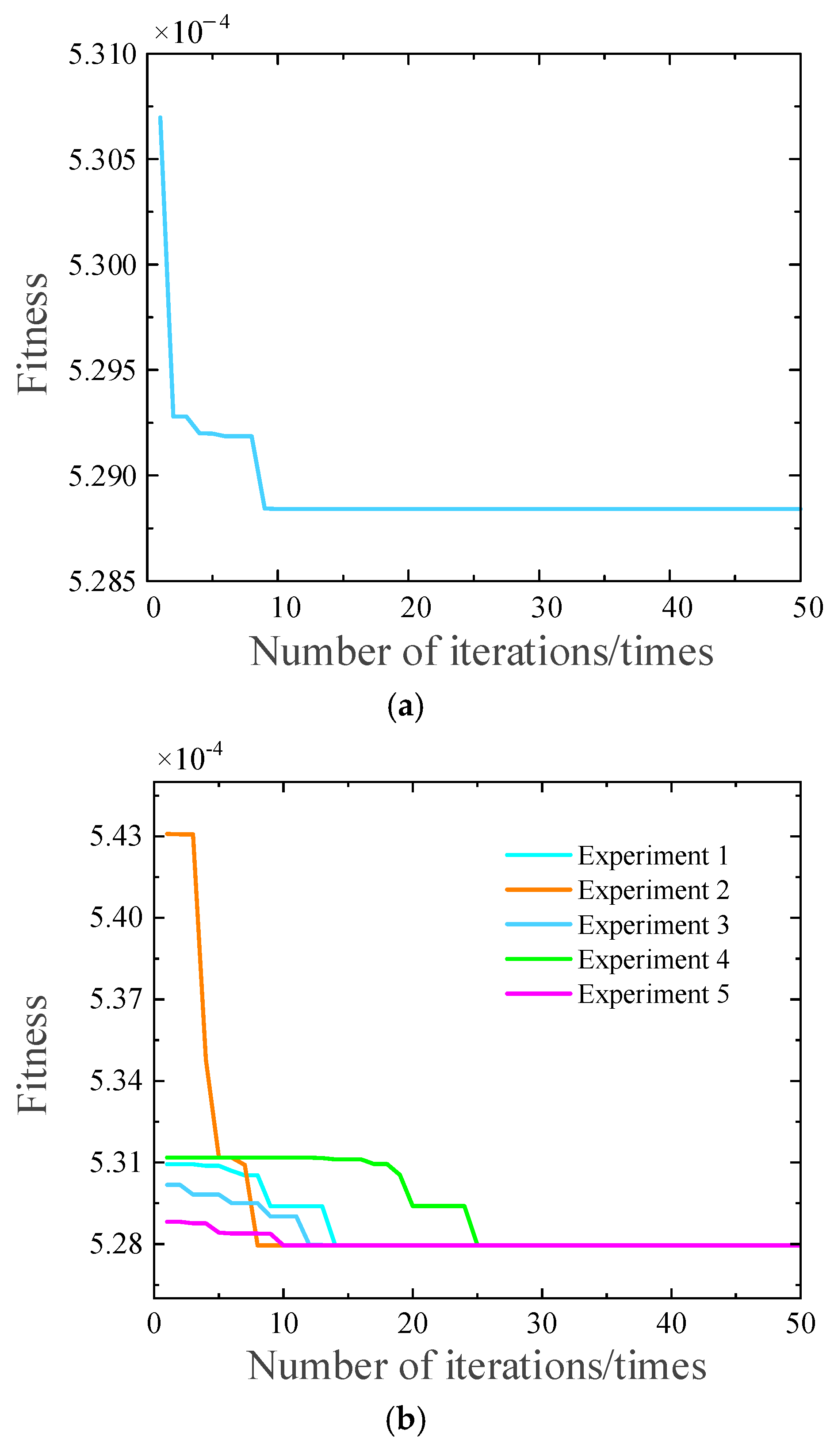
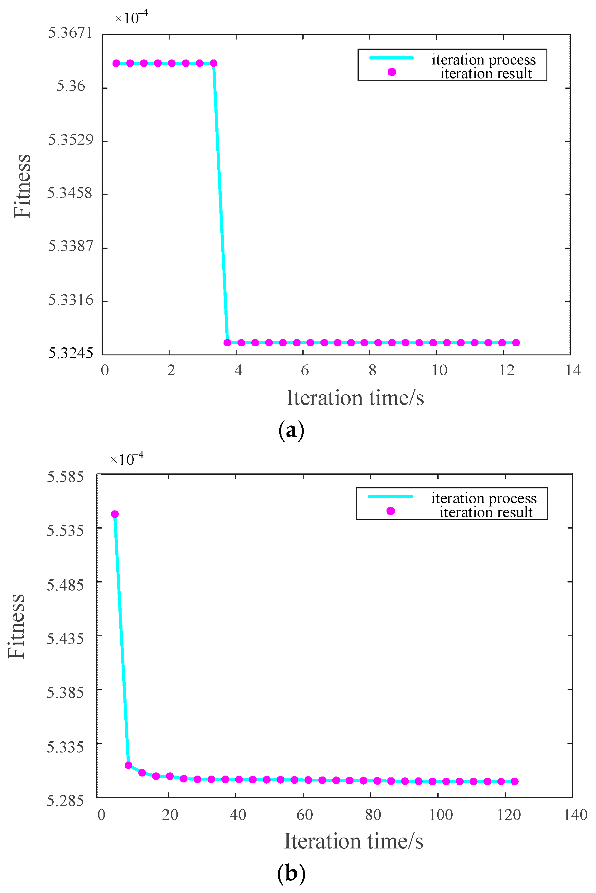
Figure 8a shows the iterative descent process of the objective function fitness of the LF-WOA. The LF-WOA reaches the threshold at the 9th generation and converges to 5.288 × 10⁻⁴.

In Figure 8a, the initial fitness value of the LF-WOA is 5.307 × 10⁻⁴. When conducting searches under the constraint of the critical threshold for key component failure in a 3P4L converter, the LF-WOA can locate key parameters with higher precision within fewer iterations.

The key parameters of the 3P4L converter were searched multiple times using the LF-WOA, and the fitness values of these multiple experiments are shown in Figure 8b. Through multiple experiments, even though the initial fitness values and the number of convergence iterations of the LF-WOA vary in each experiment, after a sufficient number of iterations, the fitness values can eventually converge to 5.288 × 10⁻⁴.

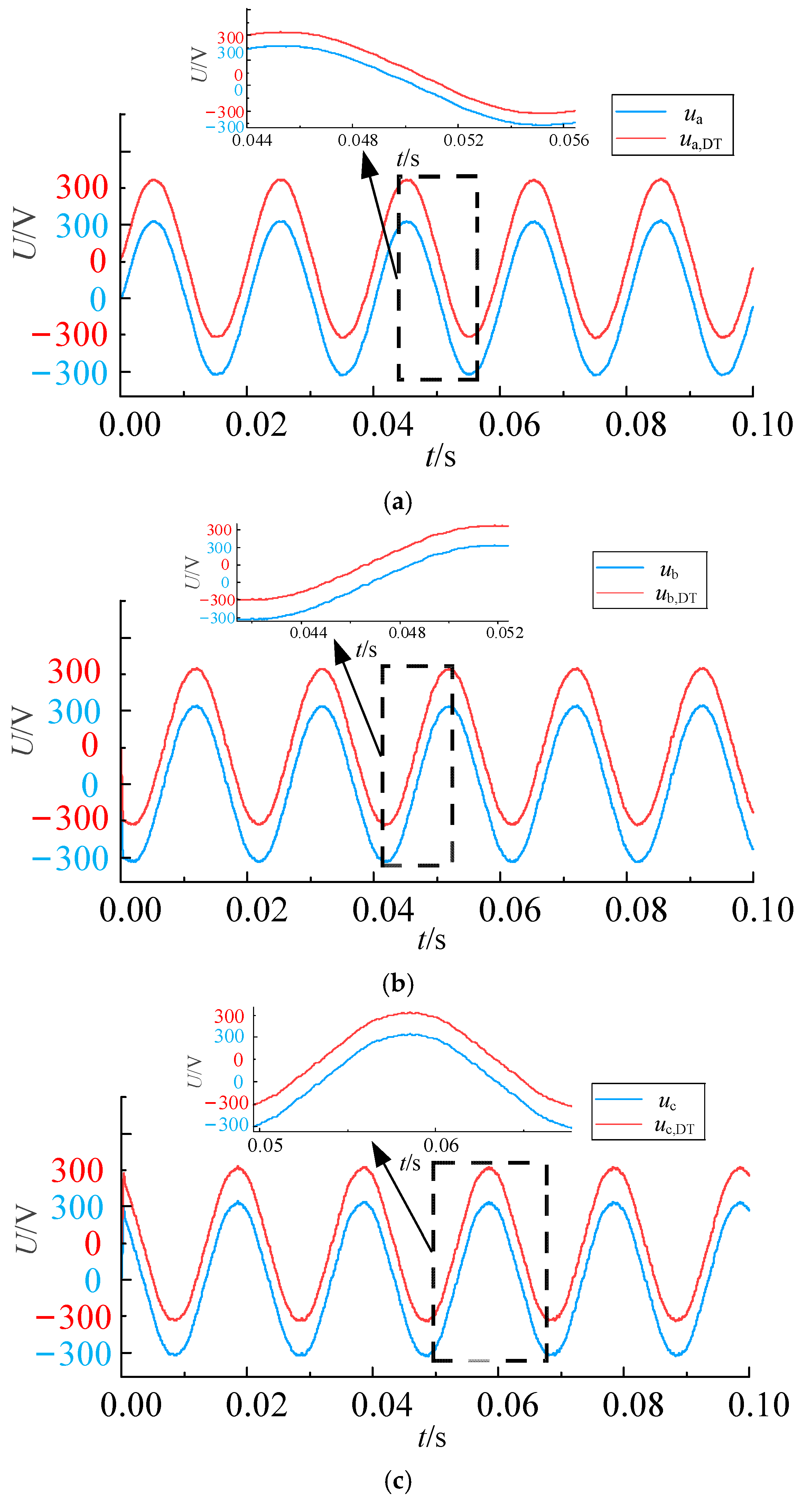
As presented in Figure 9, the waveforms of the three-phase output voltage and current from the digital twin and simulation model of the 3P4L converter are compared. It can be observed that significant discrepancies exist between the digital twin and simulation model waveforms when the LF-WOA starts the optimization process. However, as the LF-WOA undergoes continuous iterative optimization, the waveforms of the two models become nearly identical, which validates that the operating conditions of the proposed 3P4L converter digital twin model are fundamentally consistent with those of the converter simulation model.

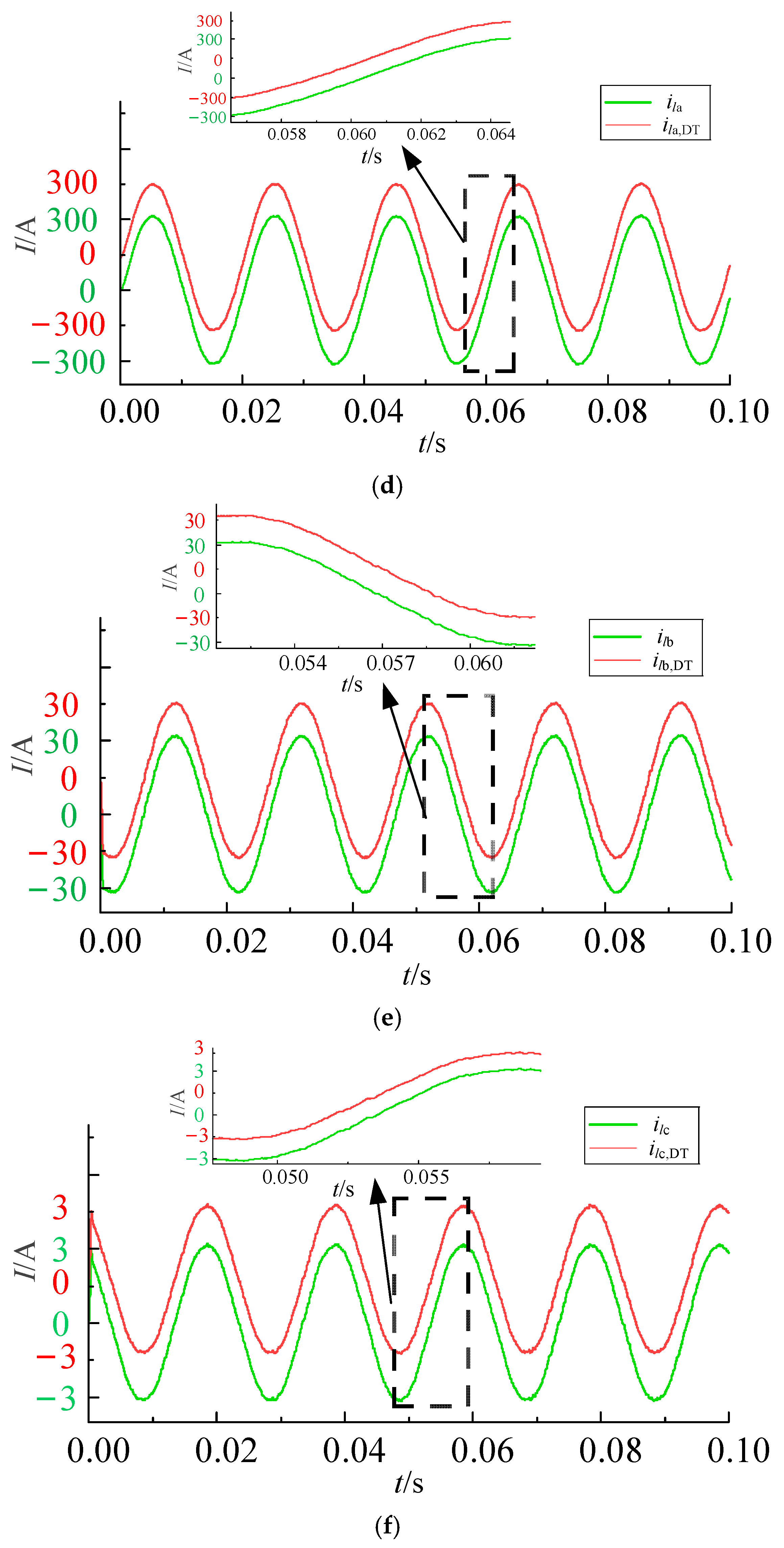
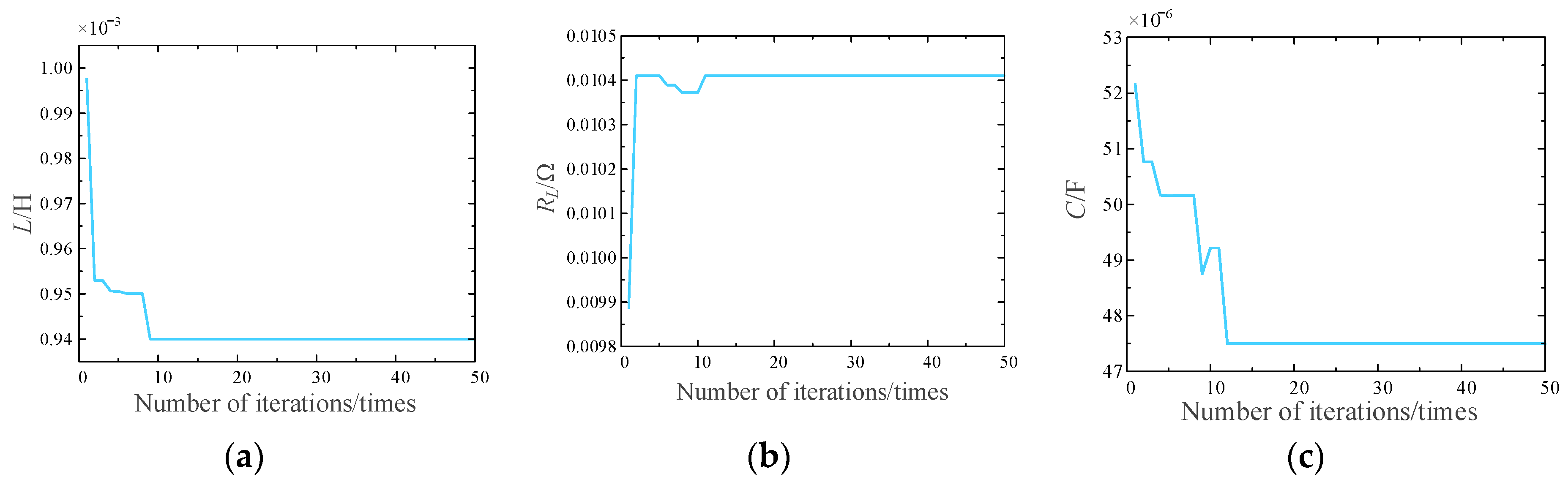
The parameter convergence results are presented in Figure 10. The parameter set (L, R_L, and C) converged to stable values after nine generations of iteration. As can be seen from

Table 6. Results and errors of parameter identification based on the simulation model.

Parameter	Identification Results	Target Value	Error
L/mH	0.94	1	6%
RL/Ω	0.01041	0.01	4.1%
C/μF	47.5	50	5%

, the LF-WOA identified the inductance of the 3P4L converter digital twin as 0.94 mH, the capacitance as 47.5uF, and the parasitic resistance of the three-phase inductors as 0.01041Ω. The identification accuracy of the three-phase inductor parasitic resistance was high, with an error of only 4.1%. While the identification errors of the filter inductor and filter capacitor were 6% and 5%, respectively, which were slightly larger than those of the inductor parasitic resistance, they remained within 10%.

4.2. Experiments on Parameter Variations

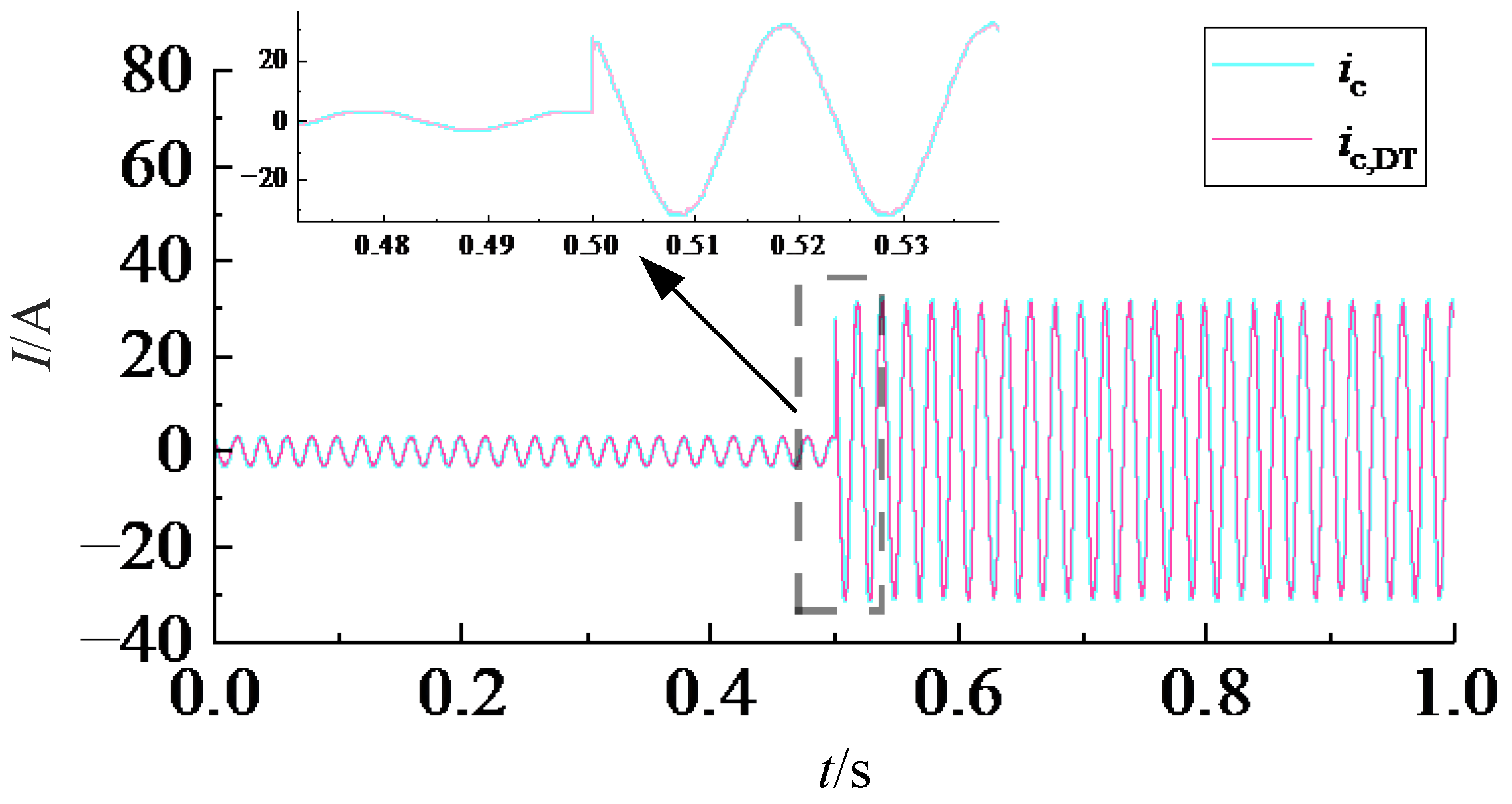
To validate the condition monitoring capability of the proposed digital twin model under sudden load changes, Figure 11 demonstrates that the phase c load is reduced from 100 Ω to 10 Ω at 0.5 s. As can be seen from Figure 12, despite the abrupt load variation in phase c, the condition monitoring results remain close to the actual values, and the operating conditions of the 3P4L converter digital twin model align nearly identically with those of the converter simulation model, indicating immunity to load changes.

4.3. Comparison of Parameter Identification Accuracies Among Multiple Optimization Algorithms

In view of the flexibility and versatility of intelligent optimization algorithms, the effectiveness of intelligent algorithms in parameter identification and the correction of internal model parameters is also verified. Scholars at home and abroad have gradually adopted intelligent optimization algorithms as parameter synchronization tools for digital twin models. However, currently, few scholars have studied the influence of different optimization algorithms on the parameter search accuracy of the digital twin models of converters. Therefore, in this section, three different optimization algorithms are employed to identify the parameters of the digital twin model of a 3P4L converter, so as to compare the search performance of different optimization algorithms when applied in the field of digital twin models.

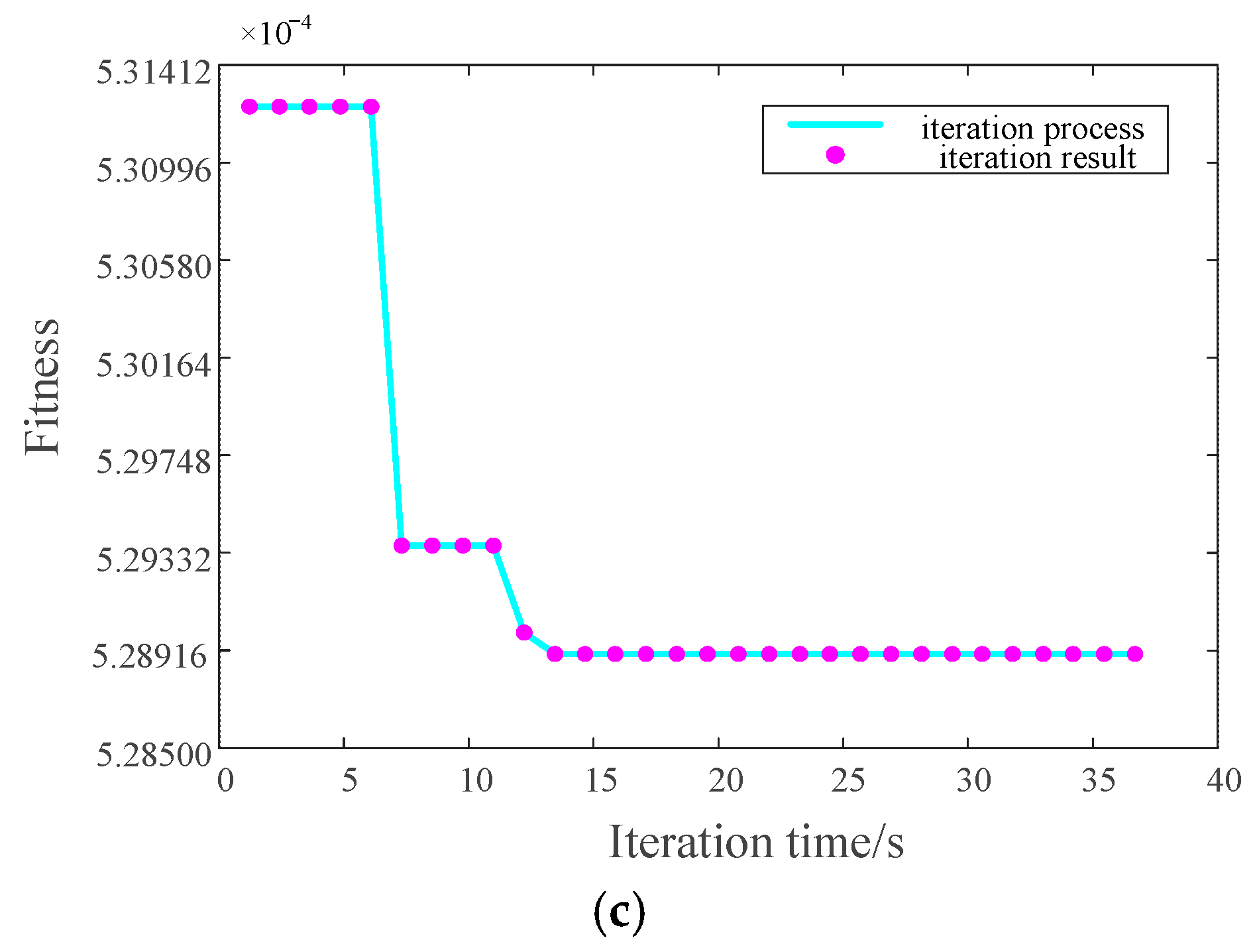
Figure 13 shows the iterative descent process of the objective functions of three optimization algorithms, namely APSO, the LF-WOA and SSA. APSO reaches the threshold after 23 iterations and converges to 5.288 × 10⁻⁴; SSA reaches the threshold after 9 iterations and converges to 5.3245 × 10⁻⁴; and the LF-WOA reaches the threshold after 11 iterations and converges to 5.288 × 10⁻⁴. From the above data, it can be seen that although SSA only needs 11 iterations to complete the search, it is obvious that SSA falls into a local optimum and fails to search for the optimal parameter set of 3P4L. Both APSO and the LF-WOA search for the optimal parameter set of 3P4L, but APSO requires 23 iterations, while the LF-WOA only needs 11 iterations to complete the task.

In this section, based on the Windows 11 operating system and with the hardware configuration of an Intel Core i9-13900KS processor, the convergence times of the three intelligent algorithms are recorded to conduct a comparative analysis of the efficiency of these three intelligent algorithms in identifying the operation characteristic parameters of a 3P4L converter.

Figure 14a–c are, respectively, the fitness–time curves of the three optimization algorithms. As can be seen from the

Table 7. Comparison of three parameter identification algorithms.

Comparison Items	SSA	APSO	LF-WOA
Convergence time consumption/s	3.74	98.4	13.45
Number of iterations/times	9	23	11
fitness	0.082247	0.082243	0.082243

, SSA takes the shortest time to complete the identification of the steady-state parameters of the converter. It only takes 3.74 s to converge. However, SSA is prone to falling into a local optimum, resulting in a relatively low identification accuracy. APSO has a relatively high parameter identification accuracy, but it takes the longest time, requiring 98.4 s to complete the convergence. Due to its mechanism of dynamically adjusting parameters, APSO transforms the parameter space from the static low-dimensional space of the traditional PSO into a dynamic high-dimensional space, leading to an increase in the time consumption. The LF-WOA can complete the convergence in only 13.45 s and achieve the fitness value that APSO takes 98.4 s to reach. Therefore, when solving high-dimensional and complex problems, the LF-WOA utilizes the spiral position update mechanism and the contraction encirclement mechanism to conduct a refined search near the current optimal solution to find a better solution. Moreover, after introducing the Levy flight strategy into the WOA, the Levy flight strategy guides the population to approach the current optimal solution and maintains a certain degree of randomness to avoid premature convergence and falling into a local optimum. As a result, the LF-WOA has a higher convergence accuracy and a faster convergence speed.

5. Hardware-in-the-Loop (HIL) Platform Validation

5.1. Verification of HIL Experiment for 3P4L Converter

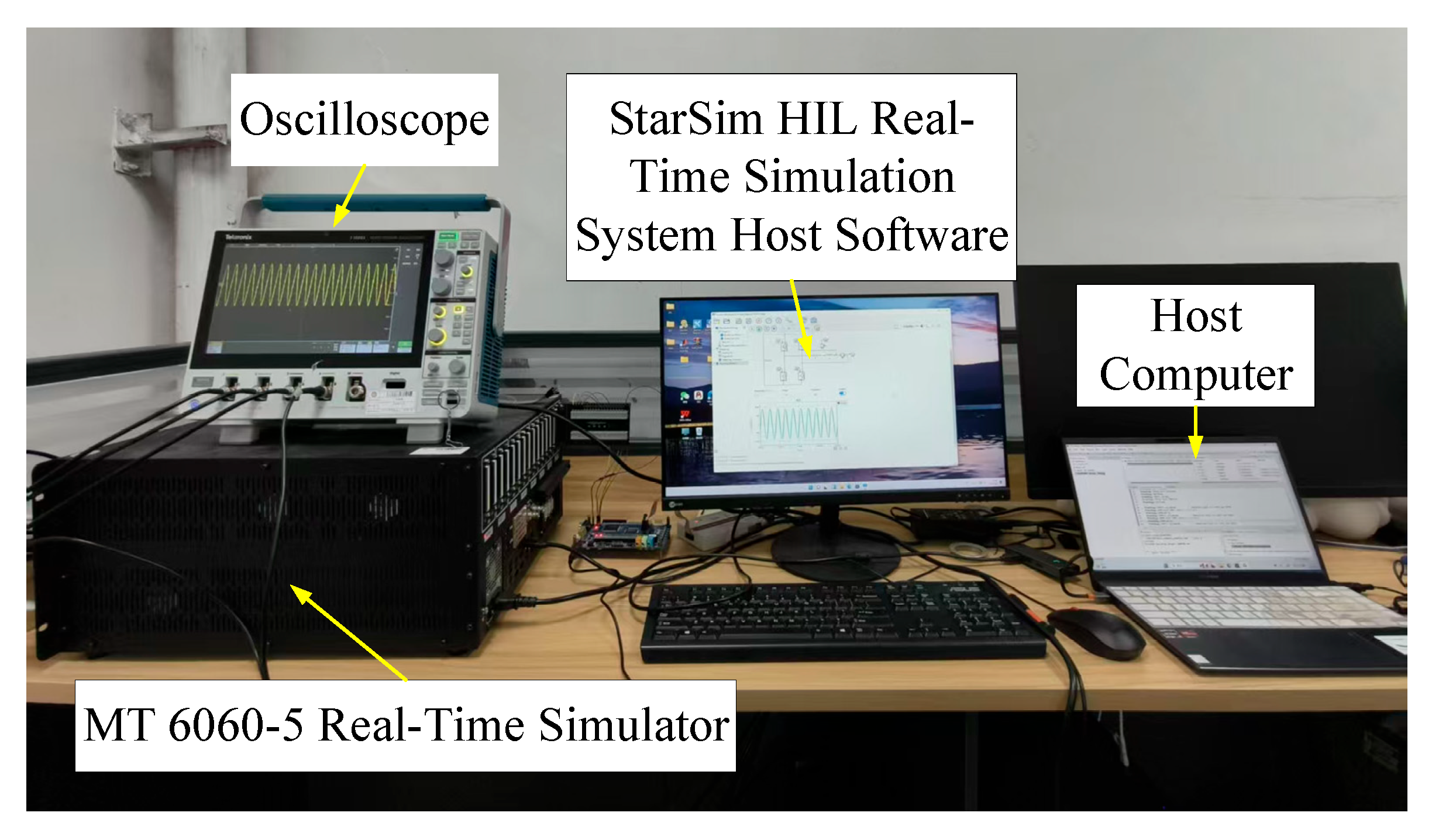
To validate the effectiveness and feasibility of the proposed method in practical converters, a StarSim HIL experimental system, as shown in Figure 15, was constructed [22]. The hardware-in-loop experimental platform consists of three components: a PC host, a StarSim real-time simulator, and an oscilloscope. The main circuit is loaded into the field-programmable gate array (FPGA) of the StarSim real-time simulator via the StarSim HIL 5.3.0 software on the host computer, with the oscilloscope used for waveform output.

The 3P4L converter has the capability to connect to external unbalanced loads. Taking linear unbalanced load conditions as an example, this paper analyzes the performance of the converter system. The linear unbalanced load configuration is as follows: phase A is connected to a 1 Ω resistive load, phase B to a 10 Ω resistive load, and phase C to a 100 Ω resistive load.

The HIL simulation experiment parameters of the 3P4L converter are presented in

Table 8. StarSim HIL platform model parameters.

Specification	Value	Threshold Range
DC bus voltage Udc	750 V	±5% to ±10% of the rated voltage
Three-phase inductance La, Lb, Lc	1 mH	within ±10%
Parasitic resistance of three-phase filter inductors RLa, RLb, RLc	0.01 Ω	within ±10%
Filter capacitor C	50 μF	from ±10% to ±20%
Equivalent series resistance of power switching devices Rdi	1 × 10−3 Ω	from ±10% to ±20%
Phase a load Ra	1 Ω	/
Phase b load Rb	10 Ω	/
Phase c load Rc	100 Ω	/
CPU-side simulation step	50 × 10−6 s	/
FPGA-side simulation step	1 × 10−6 s	/

.

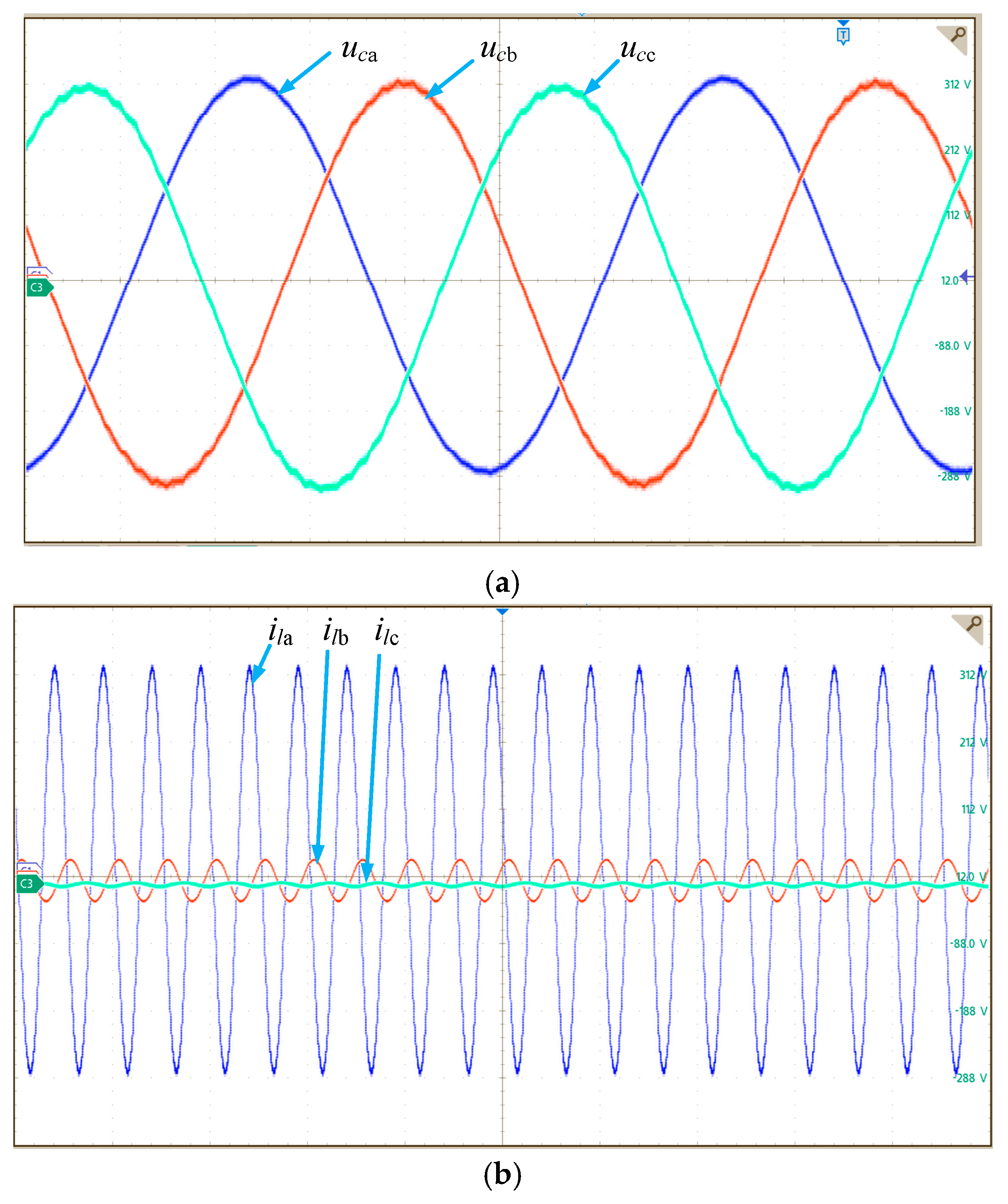
Figure 16 illustrates the voltage and current waveforms of the 3P4L converter with an external unbalanced load in the StarSim self-closed-loop system. After phase a is loaded, the output voltage peak reaches 315 V, and the voltage peaks of phases B and C are nearly identical to those of phase a.

As shown in Figure 17, the target function descent process demonstrates that with the LF-WOA iteratively optimizing, the algorithm terminates iteration and converges to the optimal value at the sixth generation.

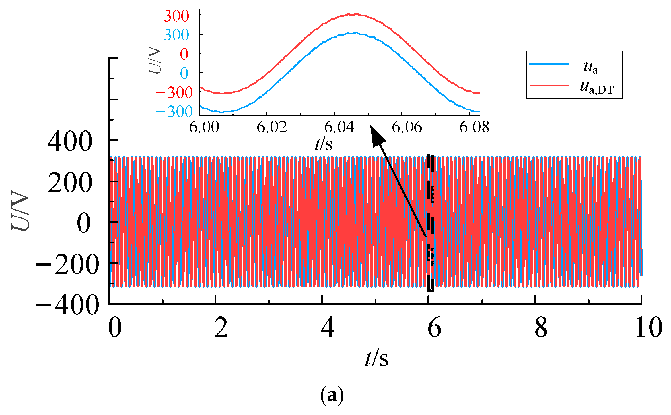
As shown in Figure 18, the waveforms of the three-phase capacitor voltage and three-phase inductor current of the digital twin of the 3P4L converter and the StarSim HIL model are compared. It can be observed from the figure that with the continuous iterative optimization of the LF-WOA, the circuit parameters of the digital twin of the 3P4L converter are getting closer and closer to those of the StarSim HIL model. When the LF-WOA converges, the waveforms of the two completely overlap. The parameter set of the 3P4L converter digital twin model constructed in this paper is almost the same as that of the StarSim HIL model, verifying that this digital twin can effectively reflect the operating state of the StarSim HIL model.

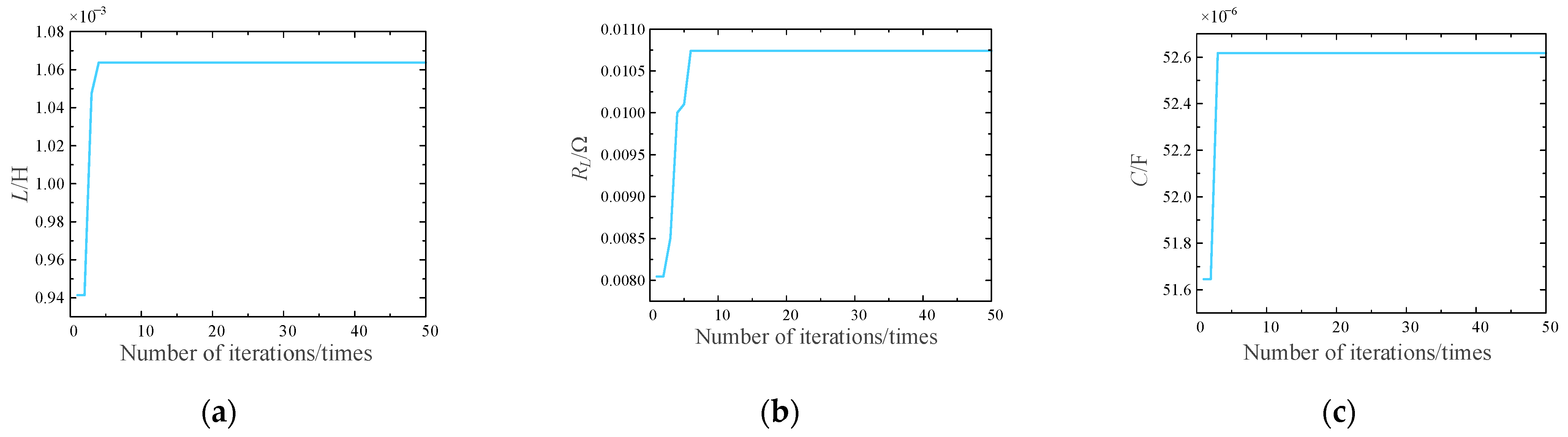
The identification process of the inductance parasitic resistance is shown in Figure 19. As can be seen from the

Table 9. Parameter identification results and errors.

Parameter	Identification Results	Target Value	Error
L/mH	1.0638	1	6.38%
RL/Ω	0.01074	0.01	7.4%
C/μF	52.618	50	5.236%

, the identified inductance value is 1.0638 mH, with a relative error of 6.38% compared to the target value. The identified parasitic resistance of the inductance is 0.01074 Ω, with a relative error of 7.4%, and the identified filter capacitor value is 52.618 μF, with a relative error of 5.236%.

The HIL experiments conducted on the StarSim platform demonstrate that the identified results of the proposed parameter identification method for the 3P4L converter are in close agreement with the target parameters, with all errors within 10%. This validates the effectiveness of the proposed method for identifying parameters of practical converter components.

5.2. Parameter Sudden Change Experiment

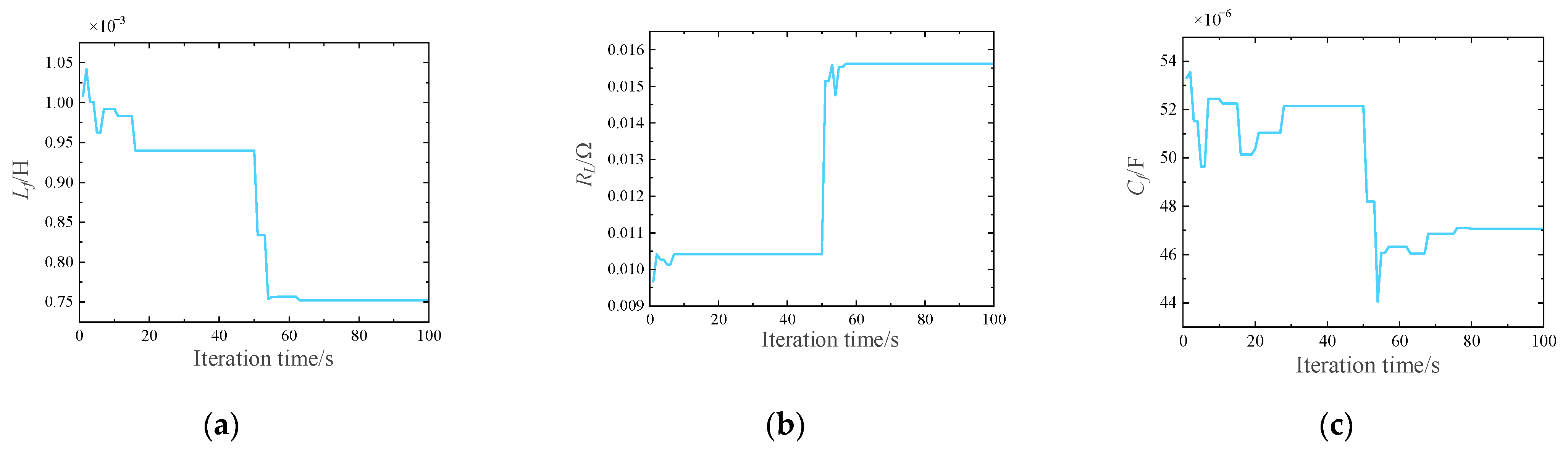
In order to verify the effectiveness of the online identification of the parameter degradation process, sudden change experiments were carried out on the characteristic parameters of the 3P4L converter at the 50th second. The inductance value decreased from 1 mH to 0.8 mH, the equivalent series resistance of the inductor changed from 0.01 Ω to 0.015 Ω, and the capacitance value decreased from 50 μF to 45 μF. The dynamic parameter identification process is shown in Figure 20.

As can be seen from the

Table 10. Summary of errors in parameter identification. 

Parameter	Identification Results Before Parameter Sudden Change	Target Value	Error	Identification Results After Parameter Sudden Change	Target Value	Error
L/mH	0.940	1	6%	0.752	0.8	6%
RL/Ω	0.0104	0.01	4%	0.0157	0.015	4.7%
C/μF	52.149	50	4.3%	47.067	45	4.6%

, before the parameter sudden change, the identification result of the inductor of the 3P4L converter was 0.94 mH, with a relative error of 6% compared to the target value. The identification result of the series equivalent resistance of the inductor was 0.0104 Ω, with a relative error of 4% compared to the target value. The identification result of the filter capacitor was 52.149 μF, with a relative error of 4.3% compared to the target value. After the parameter sudden change, the identification result of the inductor was 0.752 mH, with a relative error of 6%. The identification result of the series equivalent resistance of the inductor was 0.0157 Ω, with a relative error of 4.7%. The identification result of the filter capacitor was 47.067 μF, with a relative error of 4.6%.

After the parameters changed, each characteristic parameter of the 3P4L converter could be quickly identified, and the relative errors of the identification results were all around 5%. Therefore, the parameter identification method of the 3P4L converter based on the digital twin proposed can accurately perform parameter identification during the transient process of the 3P4L converter.

6. Conclusions

This paper presents a digital twin model-based multi-parameter coordinated identification method for 3P4L converters. First, an equivalent simplified model is established according to its circuit topology and physical operation mechanism. The digital twin model is built by solving the RK4 method, and the LF-WOA is employed to identify the characteristic parameters of the digital twin. Finally, a Matlab-based simulation and StarSim-based hardware-in-loop experiment platforms are conducted to validate the proposed method. The simulation and hardware-in-loop experimental results demonstrate that this method can achieve multi-parameter accurate identification without external hardware calibration, providing a practical solution for the state detection and health management of 3P4L converters.

References

Kong, W.; Ma, K.; Wu, Q. Three-Phase Power Imbalance Decomposition Into Systematic Imbalance and Random Imbalance. IEEE Trans. Power Syst.2018, 33, 3001–3012. [Google Scholar] [CrossRef]
Tang, C.-Y.; Jheng, J.-H. An Active Power Ripple Mitigation Strategy for Three-Phase Grid-Tied Converters Under Unbalanced Grid Voltages. IEEE Trans. Power Electron.2023, 38, 27–33. [Google Scholar] [CrossRef]
Zhou, F.; Chen, X.D.; Shi, H.R.; Yang, C.; Zhou, S.Q.; Hao, T. Research on Three-Phase Unbalance Control of Low-Voltage Distribution Network Based on Load Commutation. J. Electr. Eng. Technol.2024, 19, 4027–4043. [Google Scholar] [CrossRef]
Li, Y.; Gao, Y.; Zhang, Y.; Liu, J.; Nie, C. Accurate SiC MOSFET Chip Extraction Based on Parasitic Parameter Impact Compensation. IEEE Trans. Power Electron.2023, 38, 3201–3212. [Google Scholar] [CrossRef]
He, S.; Yu, M.; Chen, Y.; Zhou, Z.; Yu, L.; Zhang, C.; Ni, Y. Prediction of IGBT Gate Oxide Layer’s Performance Degradation Based on MultiScaleFormer Network. Micromachines2024, 15, 985. [Google Scholar] [CrossRef]
Pang, L.; Zhang, T.-Y.; Zhang, K.; Liu, L. Parameter Identification of Key Components of Thyristor Converter Valve Based on Wavelet Packet Key Feature Extraction and Elman Neural Network. IET Gener. Transm. Distrib.2022, 17, 947–961. [Google Scholar] [CrossRef]
Liu, Y.; Qing, X.; Chen, G. One-Cycle Digital Twin-Based Multiparameter Identification of Power Electronic Converters with Simple Implementation and High Accuracy. IEEE Trans. Instrum. Meas.2024, 73, 3537311. [Google Scholar] [CrossRef]
Mayer, A.; Greif, L.; Häußermann, T.M.; Otto, S.; Kastner, K.; El Bobbou, S.; Chardonnet, J.-R.; Reichwald, J.; Fleischer, J.; Ovtcharova, J. Digital Twins, Extended Reality, and Artificial Intelligence in Manufacturing Reconfiguration: A Systematic Literature Review. Sustainability2025, 17, 2318. [Google Scholar] [CrossRef]
Hu, K.; Liu, Z.; Iannuzzo, F.; Blaabjerg, F. Simple and Effective Open Switch Fault Diagnosis of Single-Phase PWM Rectifier. Microelectron. Reliab.2018, 88–90, 423–427. [Google Scholar] [CrossRef]
Yong, C.; Zhang, J.; Chen, Z. Current Observer-Based Online Open-Switch Fault Diagnosis for Voltage-Source Converter. ISA Trans.2020, 99, 445–453. [Google Scholar] [CrossRef]
Wu, T.; Yang, F.; Farooq, U.; Li, X.; Jiang, J. An Online Learning Method for Constructing Self-Update Digital Twin Model of Power Transformer Temperature Prediction. Appl. Therm. Eng.2024, 237, 121728. [Google Scholar] [CrossRef]
Peng, Y.; Zhao, S.; Wang, H. A Digital Twin Based Estimation Method for Health Indicators of DC–DC Converters. IEEE Trans. Power Electron.2021, 36, 2105–2118. [Google Scholar] [CrossRef]
Nezio, G.D.; di Benedetto, M.; Lidozzi, A.; Solero, L. DC-DC Boost Converters Parameters Estimation Based on Digital Twin. IEEE Trans. Ind. Appl.2023, 59, 6232–6241. [Google Scholar] [CrossRef]
Zhang, S.; Song, W.; Cao, H.; Tang, T.; Zou, Y. A Digital-Twin-Based Health Status Monitoring Method for Single-Phase PWM Rectifiers. IEEE Trans. Power Electron.2023, 38, 14075–14087. [Google Scholar] [CrossRef]
Wileman, A.J.; Aslam, S.; Perinpanayagam, S. A Component Level Digital Twin Model for Power Converter Health Monitoring. IEEE Access2023, 11, 54143–54164. [Google Scholar] [CrossRef]
Guzman Razo, D.E.; Madsen, H.; Wittwer, C. Genetic Algorithm Optimization for Parametrization, Digital Twinning, and Now-Casting of Unknown Small- and Medium-Scale PV Systems Based Only on on-Site Measured Data. Front. Energy Res.2023, 11, 1060215. [Google Scholar] [CrossRef]
Boldo, S.; Faissole, F.; Chapoutot, A. Round-Off Error and Exceptional Behavior Analysis of Explicit Runge-Kutta Methods. IEEE Trans. Comput.2020, 69, 1745–1756. [Google Scholar] [CrossRef]
Mirjalili, S.; Lewis, A. The Whale Optimization Algorithm. Adv. Eng. Softw.2016, 95, 51–67. [Google Scholar] [CrossRef]
Bernardeau, F.; Pichon, C. The Statistics of Rayleigh-Levy Flight Extrema. Astron. Astrophys. (A&A)2024, 689, 21. [Google Scholar]
Mantegna, R.N. Fast, Accurate Algorithm for Numerical Simulation of L’evy Stable Stochastic Processes. Phys. Rev. E1994, 49, 4677. [Google Scholar] [CrossRef]
Yang, X.-S.; Deb, S. Eagle Strategy Using Lévy Walk and Firefly Algorithms for Stochastic Optimization. In Nature Inspired Cooperative Strategies for Optimization (NICSO 2010); González, J.R., Pelta, D.A., Cruz, C., Terrazas, G., Krasnogor, N., Eds.; Springer: Berlin/Heidelberg, Germany, 2010; pp. 101–111. ISBN 978-3-642-12538-6. [Google Scholar]
Li, M.; Geng, H.; Zhang, X. Distributed Coordinated Control for Stabilization of Multi-Converter Power Plant. IEEE Trans. Ind. Electron.2023, 70, 12421–12430. [Google Scholar] [CrossRef]
Figure 1.
The 3P4L converter.
Figure 2.
Average model of 3P4L converter in stationary coordinate system.
Figure 4.
A flowchart of the control implementation for 3P4L converters.
Figure 5.
A switching vector diagram of the 3P4L converter in the stationary coordinate system.
Figure 7.
Construction framework of digital twin model for 3P4L converters.
Figure 8.
LF-WOA objective function descent process. (a) LF-WOA objective function descent process; (b) fitness comparison plot across multiple experiments.
Figure 9.
Comparison of waveforms between digital twin and simulation models for 3P4L converter. (a) Comparison of phase a voltage waveforms for 3P4L converter; (b) comparison of phase b voltage waveforms for 3P4L converter; (c) comparison of phase c voltage waveforms for 3P4L converter; (d) comparison of phase a current waveforms for 3P4L converter; (e) comparison of phase b current waveforms for 3P4L converter; (f) comparison of phase c current waveforms for 3P4L converter.
Figure 10.
Parameter identification results of the 3P4L converter. (a) Results of the inductive identification; (b) results of the inductor resistance identification; (c) results of the capacitance identification.
Figure 11.
Sudden load change current waveforms of 3P4L converter.
Figure 12.
Phase c current monitoring results.
Figure 13.
The iterative descent process of the objective functions of APSO, the LF-WOA and SSA.
Figure 16.
P4L converter output waveforms on starsim platform. (a) three-phase voltage waveform diagram; (b) three-phase current waveform diagram.
Figure 17.
LF-WOA fitness descent curve.
Figure 18.
Comparison of waveforms between digital twin and starsim platform for 3P4L converter. (a) Comparison of phase a voltage waveforms for 3P4L converter; (b) comparison of phase a voltage waveforms for 3P4L converter (partial enlarged view); (c) comparison of phase b voltage waveforms for 3P4L converter; (d) comparison of phase b voltage waveforms for 3P4L converter (partial enlarged view); (e) comparison of phase c voltage waveforms for 3P4L converter; (f) comparison of phase c voltage waveforms for 3P4L converter (partial enlarged view); (g) comparison of phase a current waveforms for 3P4L converter; (h) comparison of phase a current waveforms for 3P4L converter (partial enlarged view); (i) comparison of phase b current waveforms for 3P4L converter; (j) comparison of phase b current waveforms for 3P4L converter (partial enlarged view); (k) comparison of phase c current waveforms for 3P4L converter; (l) comparison of phase c current waveforms for 3P4L converter (partial enlarged view).
Figure 19.
StarSim HIL platform parameter identification results. (a) Results of inductive identification; (b) results of inductor resistance identification; (c) results of capacitance identification.
Figure 20.
The results of parameter identification in the parameter sudden change experiment. (a) The results of the inductive identification; (b) the results of the inductor resistance identification; (c) the results of the capacitance identification.