Q-Learning Approach Applied to Network Security

Abstract

Network security and intrusion detection and response (IDR) are necessary issues nowadays. Enhancing our cyber defense by discovering advanced machine learning models, such as reinforcement learning and Q-learning, is a crucial security measure. This study proposes a novel intrusion response method by implementing an off-policy Q-learning approach. We test the validity of our model by conducting a goodness-of-fit analysis and proving its efficiency. By performing sensitivity analysis, we prove that it is possible to protect our network successfully and establish an immediate response mechanism that could be successfully implemented in intrusion response (IR) systems.

1. Introduction

With the evolution of Artificial Intelligence (AI), our society faces unique, unknown cyber-attacks and challenges. Therefore, we must seek contemporary methods and security mechanisms to protect our systems. Reinforcement learning has been successfully applied in robotics; numerous researchers are interested in its application in network security and, more precisely, in intrusion detection (ID) and intrusion response (IR) systems. The primary benefit of reinforcement learning is the opportunity for a decision agent to interact with the environment and acquire a reward or a penalty from it. After receiving this feedback, the agent can learn from his mistakes, adjust his behavior, and make an optimal decision based on some expected rewards. The environment is represented as a Markov Decision Process (MDP), where the agent finds himself in a particular state, takes action, receives feedback, and transitions to another state. This study aims to provide an automated intrusion response mechanism that could complement the currently developed machine learning methods for intrusion detection systems and enhance the system’s security. The study focuses on creating a conceptual module with a practical simulation and implication that will advance the existing IDRS. The objective of the ID is to locate unusual or suspicious network property behavior in a particular system. Conventional approaches focus on signatures of known attacks and compare traffic against these signatures, but cannot identify new attack types using other signatures. Anomaly detection methods can resolve this problem and do not require preliminary signature knowledge. Those approaches begin by analyzing a time-series sequence of features categorized as “normal” or “attack”. The prevalence of studies is consolidated around network-based IDS, and minimal research has been conducted on what to do next once an anomaly has been detected. In this work, we aim to administer these existing methods in conjunction with providing an automated machine learning mechanism for the subsequent steps that could be undertaken once anomaly detection has occurred. This actual reinforcement learning mechanism works in the environment of the intrusion response mechanism. It observes network control protocols and the overall health of the network and, based on IDS signals, automatically takes proper actions to handle malicious or unauthorized activities by stopping them from deteriorating and returning the system. It takes action against malicious traffic in an automated manner without requiring administrative or human intervention. Our contribution is the representation of the probabilistic structure of the intrusion response model as a Markov Decision Process, and provides a realistic implementation of Q-learning in the IR system. The analytical part of the paper provides evidence that this probabilistic structure is plausible and efficient, and its implementation could enhance security and offer a comprehensive, adaptable, automated machine learning solution to cybersecurity’s rapidly evolving environment. First, we provide relevant literature on the RL applied to IDRS in network security. We then describe conceptually the main algorithmic structure of the Q-learning model selected for our IR mechanism and outline the proposed algorithm’s application to network security. Results are reported and compared to value iteration, policy iteration, and linear programming RL methods. Ultimately, we will discuss some limitations and potential future improvements that could provide a more realistic and profound understanding of using the Q-learning approach in network security.

2. Literature Review

Intrusion detection methods are widespread in the network security literature. Their goal is to detect attacks and deviations in network traffic. Traditional approaches are based on comparing the evaluated traffic with known signatures. This approach is a misuse detection method unsuitable for encountering unseen attacks [1].

The anomaly detection methods do not need any previous details of particular signatures and can find new attacks. However, they deal with a lot of noise and uncertainty and, therefore, have elevated false-positive rates. A preliminary element of the IDS is an element received from a sensor at a given time; this could be either a system call in-host-based IDSs or a feature in network-based IDSs. A series of anomaly detection is a time-series sequence of features classified as normal or abnormal. In [2], Cannady proposes a modified reinforcement learning method for employing adaptive neural networks to ID. The author analyzes the denial-of-service (DOS) attacks employing a cerebellar model articulation controller (CMAC) neural network (Albus, 1975). The first stage starts with training the CMAC with simulated attacks, followed by a single test iteration. Three hundred DoS attacks are tested, and the least mean square learning is used to update the weights of CMAC. The reported error was 3.24%. In the second stage, the adaptive learning capabilities of the model are tested to identify differences from DoS attacks. The CMAC is evaluated based on the initial performance before and after receiving feedback from the environment. Before receiving input from the environment, the reported model error is 15.2%, and after that, it improves to 0.4%. Based on the results, the author claims that the CMAC model can obtain meaningful and rapid learning for known and unknown attacks and perform online adaptive learning with significant accuracy.

Another category is based on the reinforcement learning policy, for which the action-value function is maximized. A policy is the proposed action that the agent takes, conditional on each state. The RL process could be categorized into on-policy and off-policy learning methods. On-policy methods use a known general policy, and after an action is selected, the model revises the value functions. After exploring and obtaining environmental feedback to optimize the action-value function, the policy may be modified.

Xu and Luo [3] propose a kernel-based RL method for sequential behavior modeling in-host-based IDSs, using system call sequences. They consider a kernel-induced feature space and least-squares temporal difference (LS-TD) algorithm. The model could be introduced as a sequential prediction case, which is resolved by utilizing reward signals. The authors empirically present excellent performance metrics of their proposed model compared to the Hidden Markov Models (HMMs) and linear TD algorithms. In order to reduce the feature space, a kernel approach is applied, where a high-dimensional nonlinear feature mapping can be created by selecting a Mercer kernel function in a reproducing kernel Hilbert space (RKHS). The kernel-based LS-TD learning algorithm produces dimensions equal to the number of state transition samples. Sukhanov, Kovalev, and Styskala [4] suggest an IDS model based on temporal-difference-based sequence anomaly detection 2 (TDSAD2). Their model differs from the classical temporal model in terms of how the transitional probabilities are estimated. The classical methods require knowing the probability distribution for the transitional probabilities. The transition probability is updated by matrix A, representing the pair transitions on dependency on previous states and the number of single states. The authors propose the primary adjustment related to estimating transitional probabilities, overcoming the weakness of previous TD approaches. They keep estimating the pair transition probabilities instead of the occurrence number and introduce the dependence on the previous entrance of observed states. They also estimate each state to reduce computational power. The so proposed method can be successfully applied to IDS.

In another paper [5] Xu proposes another anomaly detection approach for sequential data founded on TD learning, where a Markov reward function is presented. The author claims that TD in reinforcement learning can successfully detect abnormal behavior in the case of elaborated sequential processes by estimating the value of the Markov reward function. The advantage of the suggested model is that there is a straightforward labelling procedure utilizing delayed signals. The accuracy can be improved even with a limited training set, and it is superior to the accuracy obtained with support vector machines (SVM) and HMMs. The performance metrics of the presented anomaly detection procedure using TD learning are estimated from a system call data of host-based ID from the MIT Lincoln Lab and the University of New Mexico (UNM). The author suggests a sequential anomaly detection approach for multistage attacks based on temporal-difference (TD) learning. A Markov reward model is created, and it is also demonstrated that the value function in the Markov reward model is analogous to the anomaly probability of the data sequences.

The off-policy methods encounter policies that optimize the action-value function during learning by utilizing unused theoretical actions. Sengupta, Sen, Sil, and Saha [6] suggest a model incorporating a Q-learning algorithm and rough set theory (RST) for IDS. The algorithm aims to achieve the highest classification accuracy by categorizing the NSL- KDD data set as ”normal” or ”anomaly”. The data are discretized by applying cut operation attributes. The Q-learning algorithm is adjusted so the decision agent can learn the optimum cut value for different attributes to attain higher accuracy. The authors present two phases of the reward: the initial and final reward matrix. The proposed algorithm lowers some of the complexity of the Q-learning and obtains 98% accuracy. The authors in [7] employ a pursuit reinforcement competitive learning (PRCL) approach [8,9] for ID. This method applies immediate reinforcement learning, where feedback is obtained at each phase after making a decision. It executes clustering in real-time with high accuracy in detecting intrusions. The proposed system consists of data preprocessing, the PRCL algorithm, and the performance evaluation phase. Three methods related to competitive clustering RL are compared, and the accuracy is recorded. Mahardhik, Sudarsono, and Barakbah [10] applied RL to detect Botnet using PRCL with further rule detection, which has reward and penalty rules to achieve a solution. Based on the empirical result, PRCL can detect Botnet accurately in real-time. PRCL uses an unsupervised dataset to cluster the Botnet and obtain accuracy; it can achieve clustering online. Otoum and Kantarci [11] suggest a wireless sensor networks (WSN) detection algorithm assuming a Q-learning method on a hybrid IDS. The authors simulated twenty sensors, WSNs, which communicate through the dynamic source routing protocol for hierarchical representation networks. The tested sensor nodes are clustered in four regions of 100 m × 100 m. Twenty sensors were selected, and the Q-learning algorithm was applied. The result outperforms other machine learning methods based on accuracy, precision, and false favorable rates. Some of the more recent authors, including [12,13] represent the network as a combination of more agents and provide a broader application of the reinforcement learning aspect.

3. Markov Decision Process (MDP) and Q-Learning

Reinforcement learning is a machine learning method that allows a particular decision entity, called an agent, to interact with the unknown environment, learn from it after receiving appropriate feedback (reward), and take actions that ultimately lead to optimal decisions. The goal agent observes and analyzes the situation and selects the best possible action based on an expected maximized return. The connection with the environment can be described as a Markov Decision Process (MDP) [14], which is based on the tuple $(S,A,P,R,\gamma )$, where S stands for the set of all possible states; A denotes a set of actions; P is a transitional probability going from one state to another; R is a reward function; and $\gamma$ is a discount factor.

A decision-making entity, named an agent, interacts with a system called an environment. At time t, the agent observes the environment to be in state $S_t\in \mathcal{S}$, where $\mathcal{S}$ represents the set of all possible states. The agent chooses an action $A_t\in \mathcal{A}$, where $\mathcal{A}$ is the set of all possible actions. Then, the agent transitions to the next state $S^{\prime }$ and receives a numeric reward $R_t\in \mathcal{R}$, where $\mathcal{R}\subset \mathbb{R}$ is the set of all possible rewards. The dynamics function controls the transition probabilities and reward distributions are governed $p:\mathcal{S}\times \mathcal{R}\times \mathcal{S}\times \mathcal{A}\to [0,1]$ where $p(s^{\prime },r|s,a)$ is the probability of transitioning to state $s^{\prime }$ and receiving reward r when the environment is in state s and the agent chooses action a. The goal is to find an optimal policy: a function $\pi :\mathcal{S}\to \mathcal{A}$ that maximizes some measure of long-term reward.

A critical segment of the reinforcement learning problem is exploring new actions or considering actions that are not optimal for the given state to explore the environment more in the hope of finding better actions. The most known strategies consider a uniform selection of actions using pseudo-random numbers independent of previous actions. This selection process may select an action comparable to earlier selected actions when logic suggests a new and as different as possible is desirable. Some techniques, such as optimistic value initialization [14], will try to avoid this problem and force the selection of unseen actions. The selection of action a given the state s is called the policy $\pi$ of the decision agent. A policy $\pi$ is the conditional probability of choosing distinct actions given each state s. Policy $\pi$ can be evaluated by creating an action-value function $q_{\pi }(s,a)$. The action-value function under policy $\pi$, with a discount factor $\gamma$ and return R at time t and episode k is

$$Q^{\pi }(s,a)=E_{\pi }[\sum _{k=0}^{\infty }{\gamma }^k{R}_{t+1+k}|S_t=s,A_t=a]$$

(1)

The discount factor’s value lies between 0 and 1. When the discount factor is set to a low value that is not zero, it implies that we prefer present rewards over future rewards. Setting the discount factor to a high value of around one implies that we prefer future rewards to immediate ones. The state-value function under policy $\pi$ is

$$V^{\pi }\left(s\right)=E_{\pi }[\sum _{k=0}^{\infty }{\gamma }^k{R}_{t+1+k}|S_t=s]$$

(2)

It represents the cumulative discounted expected return for each episode k at a time t, conditional on the states $S_t=s$ that the agent needs to explore and the possible corresponding actions he has to take. The goal is to obtain the function’s maximum across all policies. This could be achieved by employing the Bellman optimality equation for the state-value function $V^{*}$ or the Bellman optimality equation for the action-value function $Q^{*}$.

$$Q^{*}(s,a)=\sum _{s^{\prime },r}P(s^{\prime },r|s,a)[R+\gamma \ast \underset{a^{\prime }}{max}q(s^{\prime },a^{\prime })]$$

(3)

The Bellman optimality equation for the state-value function $V^{*}$ is

$$V^{*}\left(s\right)=\underset{a}{max}\sum _{s^{\prime },r}P(s^{\prime },r|s,a)[R+\gamma \ast V^{*}\left(s^{\prime }\right)]$$

(4)

The Q-learning off-policy method [15] is the most popular RL off-policy procedure employed in the ID domain. It is found in the idea for value iteration, where the agent estimates the action-value function to update all states s and actions a for every iteration. The goal is to optimize the Bellman equation by taking higher rewards R actions. The equation below denotes the Q-value where $\alpha$ is a learning rate, and a constant $0<\alpha <1$ and $\gamma$ is again a discount factor $0<\gamma <1$.

$$Q^{\prime }(S_t,A_t)\leftarrow (1-\alpha )Q^{\prime }(S_t,A_t)+\alpha [R_t+\gamma max(S_t^{\prime },A_t^{\prime })]$$

(5)

The motivation for employing Q-learning as one of the top RL methods applied to ID is that it is model-free. The researchers can use the rewards as a controlling tool. Last but not least, as we mentioned before, it is an off-policy approach because it learns the model without following a particular policy [16].

4. Results

We evaluated the performance of Q-learning for intrusion detection response. Unlike the regular machine learning methods limited to intrusion detection and classification, the Q-learning method can create an intrusion response mechanism. We developed a Q-learning model to train an agent that learns the actions that maximize the action-value function for various network conditions. The agent aims to improve the response by determining the actions that maximize his expected reward.

4.1. Setting up the Environment as an MDP

We started by representing the network environment as MDP. We simulated the environment using Python 3.13.3 and predefined the actions, states, rewards, and discount factor. We do not need to define any transition probabilities for the Q-learning algorithm to work. For the agent, the different states will be represented by whether the network is under normal conditions or one of the possible types of attacks. For this example, we will consider five types of network conditions: normal traffic, denial of service (Dos), probe, root-to-local (R2L), and user-to-root (U2R) attacks.

The denial of service (DoS) cyberattack occurs when the network becomes unreachable to its legitimate users because the system is overwhelmed with traffic. These attacks can disrupt the normal functioning of online services and applications, resulting in substantial downtime and potential financial losses. Probe attacks are network observation activities in which an unauthorized entity sends distinct packets to our network so they can gather information about our system and possible vulnerabilities. Root-to-local (R2L) attacks are intrusions into our system. An unauthorized entity accesses our network by using our vulnerabilities to gain access and then transmitting packets to a remote machine. User-to-root (U2R) attacks occur when an authorized, nonprivileged user explores the system’s vulnerabilities to obtain elevated rights, such as administrator privileges, and take control.

• State space S is a countable set of states $S:\{s_N,s_{DoS},s_{probe},s_{R2L},s_{U2R}\}$; $s_N$ represents the state if the traffic is normal; $s_{DoS}$ represents the state if the traffic is under denial of service attack; $s_{probe}$ represents the state if the traffic is under a $Probe$ attack; $s_{R2U}$ represents the state if the traffic is under a $RoottoLocal$ attack; and $s_{U2R}$ represents the state if the traffic is under a $UsertoRoot$ attack, $\forall s\in \mathcal{S}$.
• Action space $A:\{a_{block},a_{report},a_{return},a_{allow}\}$, $a_{block}$ is the action to block the traffic, $a_{report}$ represents the action to report the traffic to the administrator, $a_{return}$ is the action to send the traffic back for another classification, and $a_{allow}$ is to allow the traffic in the system, $\forall a\in \mathcal{A}$.
• Transition Probability Matrix (P): This is the probability of moving from one state to another by taking a particular action; the q-learning agent learns the transition probabilities in finding an optimal policy, which is the state transition probability. Since we have four actions, for each action, we need a $5\times 5$ matrix, For example, for the action $block$, the following matrix could be represented as follows:

  $${P_{ij}}^{block}:\left[\begin{array}{ccccc}{P^{block}}_{normal,normal}& {P^{block}}_{normal,DoS}& {P^{block}}_{normal,Probe}& {P^{block}}_{normal,R2L}& {P^{block}}_{normal,U2R}\\ {P^{block}}_{DoS,normal}& {P^{block}}_{DoS,DoS}& {P^{block}}_{DoS,Probe}& {P^{block}}_{DoS,R2L}& {P^{block}}_{DoS,U2R}\\ {P^{block}}_{Probe,normal}& {P^{block}}_{Probe,DoS}& {P^{block}}_{Probe,Probe}& {P^{block}}_{Probe,R2L}& {P^{block}}_{Probe,U2R}\\ {P^{block}}_{R2L,normal}& {P^{block}}_{R2L,DoS}& {P^{block}}_{R2L,Probe}& {P^{block}}_{R2L,R2L}& {P^{block}}_{R2L,U2R}\\ {P^{block}}_{U2R,normal}& {P^{block}}_{U2R,DoS}& {P^{block}}_{U2R,Probe}& {P^{block}}_{U2R,R2L}& {P^{block}}_{U2R,U2R}\end{array}\right]$$
• Reward (R): These are the incentives for good decisions and penalties for mistakes. The reward function helps the agent move in the desired direction, ideally based on a predetermined cost function associated with the agent’s costs. The current reward values are selected based on how we would like to train the model and what we ultimately want the agent to achieve, making the agent move in this direction, as the intuition behind reinforcement learning suggests.

  $$R:\left[\begin{array}{ccccc}& a_{allow}& a_{report}& a_{return}& a_{block}\\ s_N& 5& 0& 1& -1\\ s_{DoS}& -5& 3& 0& 10\\ s_{Probe}& 0& 1& 2& 5\\ s_{R2L}& -2& 1& 4& 6\\ s_{U2R}& -3& 0& 3& 8\end{array}\right]$$
• Discount factor $\gamma$: The discount factor makes the agent far-sighted or narrow-sighted. It also helps the Q-learning converge and provides the action that maximizes the Bellman Equation (3) for the action value function. Later, we will provide a discrepancy analysis on the different levels of discount factors.

Initially, the decision agent finds himself in a particular state and knows whether it is a specific type of attack or a particular type of attack; then, he models the environment as an MDP and applies the Q-learning approach. We will test the model for different levels of the discount factors, and the goal will be to find an optimal policy that depends on the state that the decision agent is in, so he can take the most appropriate action. The optimal policy will provide the agent with the most suitable response that will optimize the Q-learning algorithm.

We use Python for training our agent and simulating the environment. The agent interacts constantly with the environment and receives feedback from it. To model the environment, we need to consider all possible states and transitions for every possible action. For example, for the action “allow”, there are five possible states, and each one of those states has five possible states to transition to; therefore, for each action, there are twenty-five possible transitions. Since there are four actions, we will observe a total of 100 possible case scenarios; the agent can find itself in any one of those options. The agent receives a corresponding reward for every possible action after transitioning from one state to another.

4.2. Q-Learning Implementation and Training Strategy

The decision agent finds itself in a particular state, selects an action, receives feedback from the environment, receives an immediate reward, and transitions to the next state. This interaction with the environment occurs over several episodes. The algorithm maintains a Q-value table to record the discounted reward expectations, and after each immediate reward that the agent receives, it updates the Q-values using the Bellman Equation (3). Firstly, a Q-table, which stores the expected reward for each state-action pair, is initialised with zeros. It is initialised with a 4 × 5 matrix due to the number of actions (4) and the number of states (5). The action-selection process is an essential part of the Q-learning algorithm because it involves a constant trade-off between exploration and exploitation. The epsilon-greedy policy provides a balanced approach to this trade-off, which is why we select it as an action selection process. At each time step, a random number is selected and compared against the epsilon $ϵ$. The agent chooses a random action if the number is less than $ϵ$. Then, he explores the environment and discovers new state-action pairs that could lead to higher rewards. Otherwise, the agent exploits the current knowledge and chooses the action with the highest Q-value for the current state, as determined by $arg{max}_{a}Q(s,a)$. As a summary, when a random action is selected with a probability $ϵ$, then the agent is in the exploration phase, and when it selects the best known action with a probability $(1-ϵ)$, then it is in the phase of exploitation. In network security, we would like our agent to find a good balance between exploration and exploitation. We would also like to ensure that it explores the environment with a high probability so it can familiarize itself with new and unseen attacks and patterns.

After taking an action, the agent receives a reward and transitions to a new state. The Q-value for the current state-action pair is then updated using the Bellman equation, which incorporates the observed reward and the maximum expected future reward from the next state.

This process is repeated across 50 steps over 300 episodes, with an average window size of 50 iterations, allowing the agent to refine its policy. Over time, the agent reduces exploration using the epsilon decay and focuses on exploiting the best policy it has learned. The Q-table stabilizes as the model converges to an optimal strategy.

4.3. Hyperparameters

To complete the process, we need to set up some parameters used in the learning process. Later, we provide a sensitivity analysis for the changes in $\gamma$ and $\alpha$, as the other parameters are required to calculate the Q-functions. $\alpha$ is the learning rate; its range is between zero and one. It also specifies how often the different Q-values will be updated, based on the feedback that the agent receives from the environment. In network security, a lower rate means that the agent will learn at a slower pace, but its decisions will be more robust and reliable. As the learning rate approaches one, the agent learns faster, which is something that the administrator may prefer in a cyber security set up. The parameter values are provided to be set by the administrator, depending on the goals of the organization and the experience. The discount factor $\gamma$ sets up the tradeoff between future and present rewards. It also guarantees that the reinforcement learning will converge. In our IR model, we may want to set up $ϵ$ closer to one. With this strategy, we would like it to explore the environment, rather than exploiting it and select the actions based on that principle. The environment in intrusion response is exclusively dynamic. A Q-learning agent must identify the most suitable response to all potential scenarios. Epsilon-greedy allows the agent to learn by trying diverse responses, applying this knowledge, and reacting effectively. The high epsilon will encourage more exploration, and later, it can decay. Besides $\alpha$ and $\gamma$ and $ϵ$ and after various executions of the model with a variety of parameter values, we concluded that the different parameters do not influence the learning capacity of the agent, and ultimately the same optimal policy is selected. We should also mention the action selection process using the $ϵ$-greedy policy.

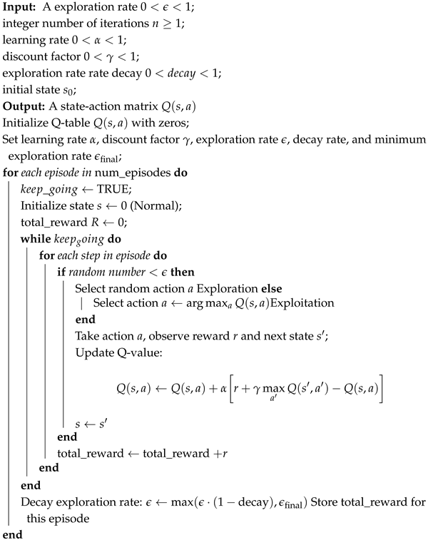
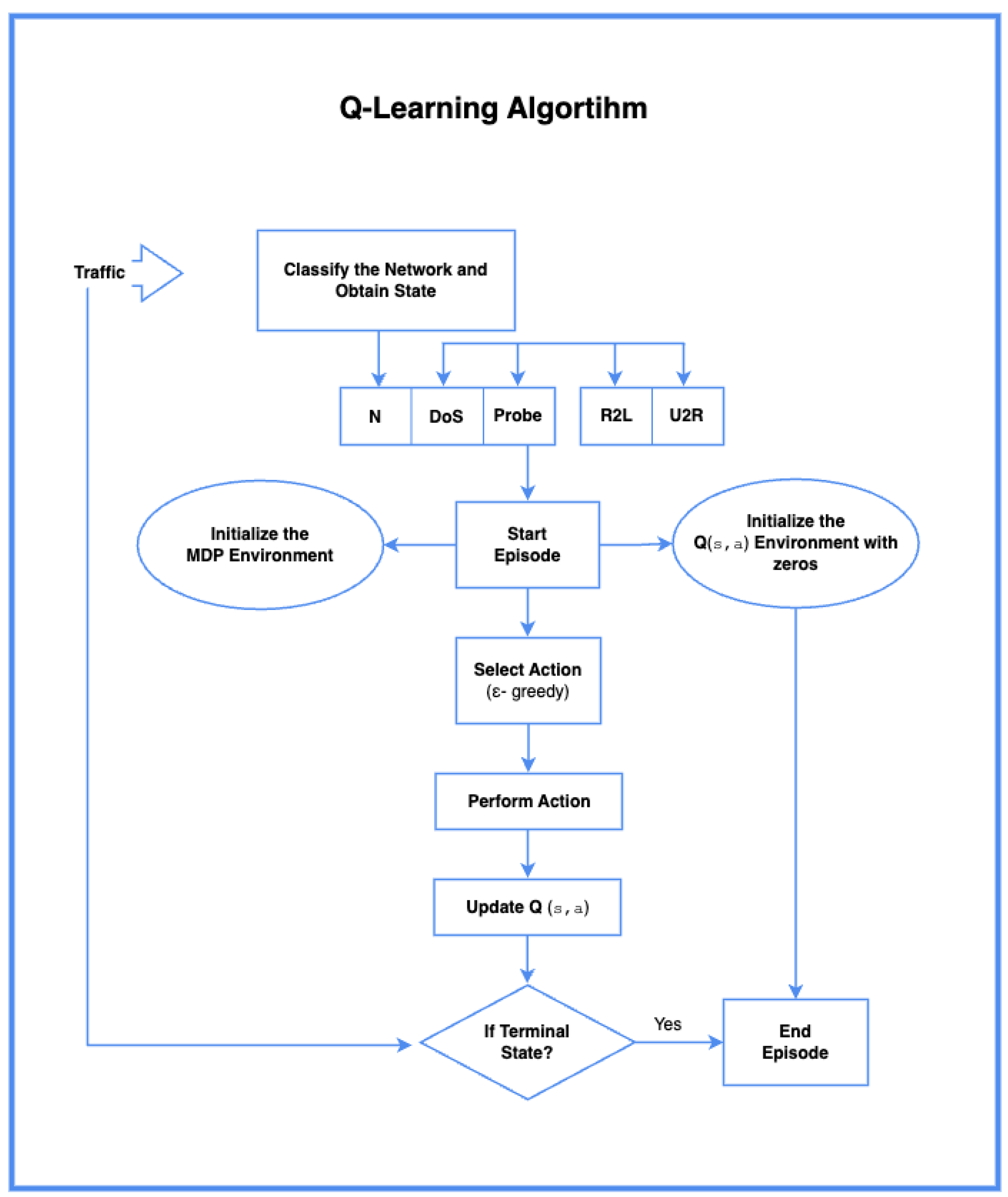
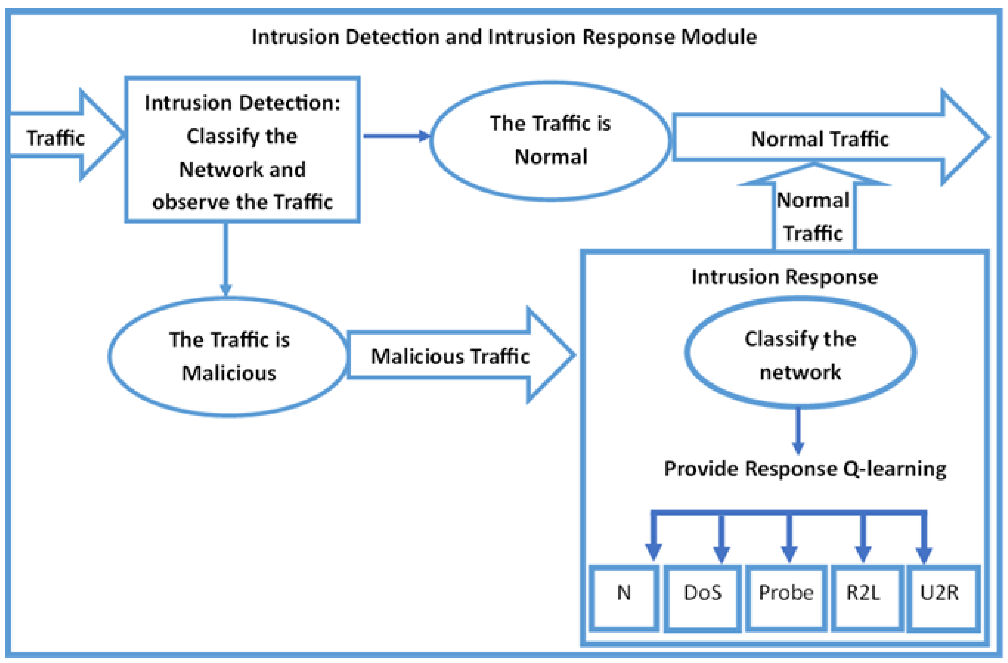
The Q-learning Algorithm 1 shown in Figure 1 begins with classifying network traffic into different categories such as N, DoS, probe, R2L, and U2R, which represent different states. The MDP environment is initialized, and the Q-values for state-action pairs are set to zero. The agent then starts the episode, selects an action using the e-greedy strategy, performs the action, and updates the Q-values based on the reward. This cycle continues until a terminal state is reached, marking the end of the episode. Through multiple episodes, the agent keeps updating its Q-values, refining its policy to learn the best actions to take in different states. The hyperparameters that we applied as an initial set-up are presented in

Table 1. Hyperparameters used in Q-learning.

Hyperparameter	Description	Value
Learning rate $\alpha$	Controls how much the weights are updated during training.	0.2
Discount factor $\gamma$	Determines the importance given to future rewards in the Q-learning equation.	0.1
Exploration rate $ϵ$	The probability of selecting a random action instead of following the learned policy.	0.9
Epsilon decay	Reduces exploration over time in favor exploitation.	0.05
Epsilon minimum	Ensures that the Q-learning agent retains a minimum level of exploration throughout training.	0.01
Number of episodes	The total number of iterations when training the agent.	200
Steps per episode	The maximum number of steps before ending an episode.	50
Moving average window	This is used to smoothen the cumulative reward over time.	30

and later we provide graphical representations for their change as well as a sensitivity analysis.

Algorithm 1: The Q-learning training algorithm

4.4. Episode Reward and Q Table

Figure 2 visualizes the training progression of a Q-learning agent over 300 episodes. It shows how the reward changes as the agent learns the optimal policy. The blue line represents the reward obtained in each episode, while the red line represents the moving average reward.

From episodes 0 to 25, the agent starts with low rewards as it has no prior knowledge of the environment. As we progress from episode 25 to 75, the agent begins to learn an effective policy, and there is a steady increase in reward. The moving average also increases consistently, indicating that the agent is discovering better decision-making strategies for intrusion detection. From episode 75, the rewards stabilize, indicating that the agent converges towards an optimal policy. The moving average reward curve flattens around episode 100, indicating that the agent has successfully learned to differentiate the different states and has selected the best action based on learned experiences. Hundred episodes in terms of network security are executed almost instantly without any delay.

Table 2. Q-table.

State	Allow	Report	Return	Block
Normal	5.57542983	0.77936266	1.58838193	−0.34863757
DoS	−4.10741098	3.92943439	0.69046204	10.88718444
Probe	0.76225638	1.76297612	2.79851319	5.71924872
R2L	−1.19494085	1.66870395	4.69743104	6.74777392
U2R	−2.24912002	0.72623961	3.84500612	8.68402438

shows the Q-Table generated after training. It represents the action-value function, the cumulative reward for each state–action pair, guiding the agent in its decision-making. The values in the table represent the long-term benefit of choosing a particular action in a state; higher values indicate more favorable conditions.

Based on those Q-values, which represent the optimal solution to the Bellman Equation (3), the agent obtains an optimal policy, and for each state, he selects the best possible action. For example, if we consider the first row of the table above, we will observe that the state the agent is currently in is “Normal” and the highest Q-value of that row is associated with the action “Allow”. Therefore, the agent will prefer to “Allow” the traffic if he is aware that the current state is “Normal”. The agent always needs to know its initial state in order for the Q-learning algorithm to work. However, he doesn’t need to estimate the transitional probabilities for the optimal solution to be provided. Therefore, Q-learning is a very suitable approach for providing optimal responses to the environment. The learning process is based on trial and error in the beginning, until the best policy is obtained. The action with the highest Q-value maximises the Q-value function and is an automotive response that could be adopted in the IR system. This outcome creates an optimal policy for the agent. This policy may or may not be unique. The next row is if the agent is under a “Dos” attack, one of the very challenging attacks for the system. The best possible action for this state, as suggested by the Q-learning algorithm, is the “Block” action. However, sometimes the best course of action is to “Report” the traffic to the administrator, because a human interaction may be preferred, especially for malicious traffic that is isolated and under “quarantine”. Continuing further, the next states in the table indicate that the best possible action is to “Block” the traffic, depending on the severity of the attack.

The sensitivity analysis of the different levels of gamma $\gamma$ (0.1, 0.3, 0.5), as well as the levels of iterations of the model, are represented in Figure 3. We plotted the moving average reward across 1000 training episodes. With a $\gamma$ value of 0.1, the model converges more quickly and stably than with 0.3 and 0.5. This indicates that 0.1 is the most favourable discount factor for intrusion response, where quick decisions are essential. The lower gamma value emphasizes immediate rewards, so the agent optimizes its policy faster without relying on a long-term reward estimation. Higher gamma values of 0.3 and 0.5 exhibit instability and delayed convergence, rendering them less suitable for environments that require prompt responses to threats. Therefore, $\gamma$ = 0.1 was selected as the optimal value for this implementation.

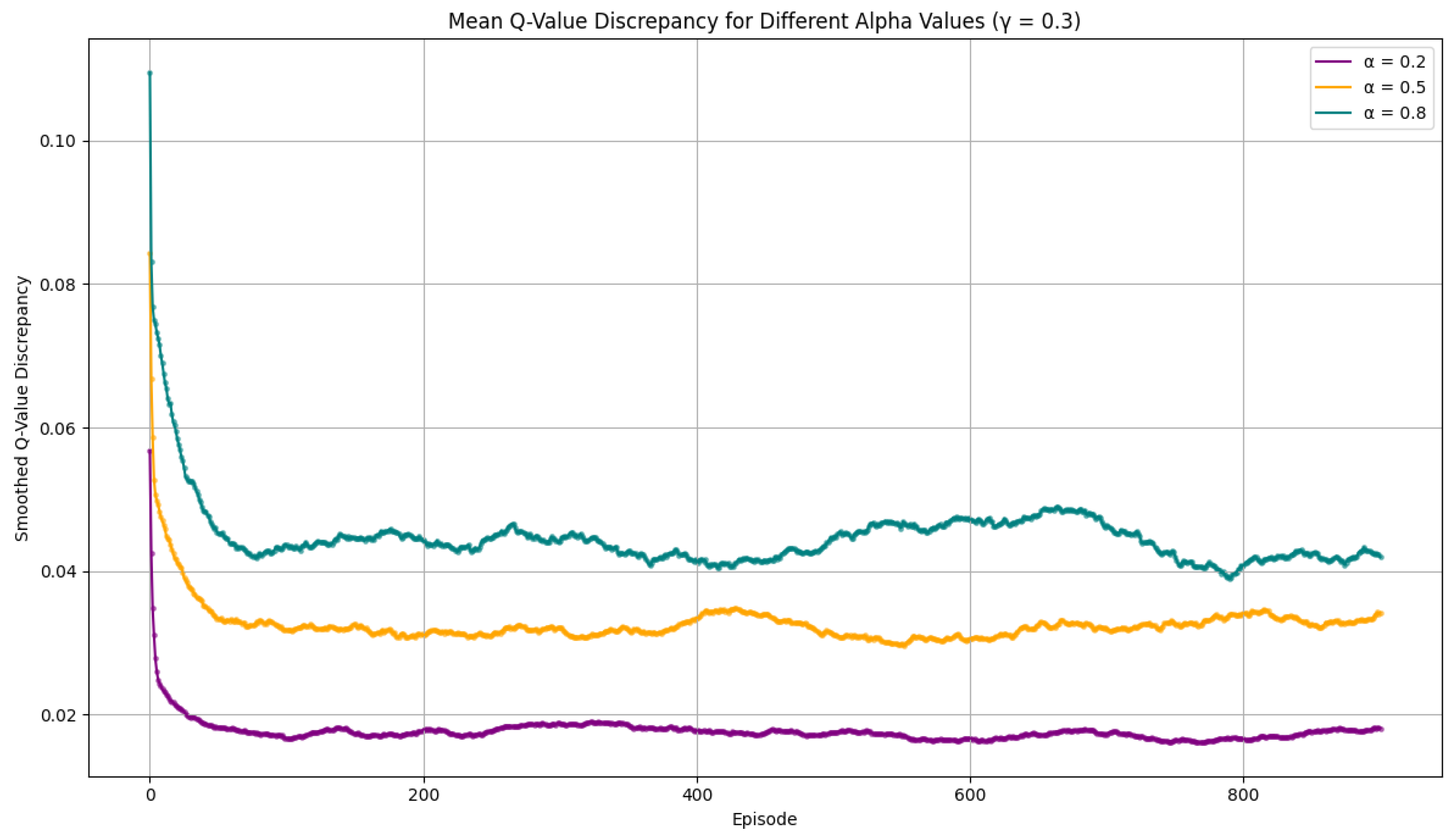
We also provided the sensitivity analysis for $\alpha$, the learning factor at different levels (0.2, 0.5, and 0.8). On Figure 4, we can observe the dynamics of the changes in the learning rate. We want to explore lower alpha values in network security because we usually observe a very time-sensitive environment. Our Q-learning model achieves excellent results at lower gamma and alpha levels, based on 1000 episodes. The alpha learning parameter in Q-learning controls the rate at which the agent updates its Q-values based on new information. It controls the importance of the new experience when updating the Q-value. A lower alpha means the agent updates its Q-policy more slowly, leading to a potentially more stable but slower convergence.

4.5. Optimal Policy

As shown in

Table 3. Optimal policy derived from Q-learning.

State	Optimal Policy
State 0 (Normal)	Allow
State 1 (DoS)	Block
State 2 (Probe)	Block
State 3 (R2L)	Block
State 4 (U2R)	Block
Cummulative Reward	330

, the optimal policy derived from the training process aligns with our goal of allowing “normal” traffic and blocking the attacks. We tested different levels of discount factors and learning rates, but the optimal policy remains to block traffic when the attack occurs. The model is very robust towards changes in all parameters.

4.6. Evaluating Q-Learning Policy on Test Episodes

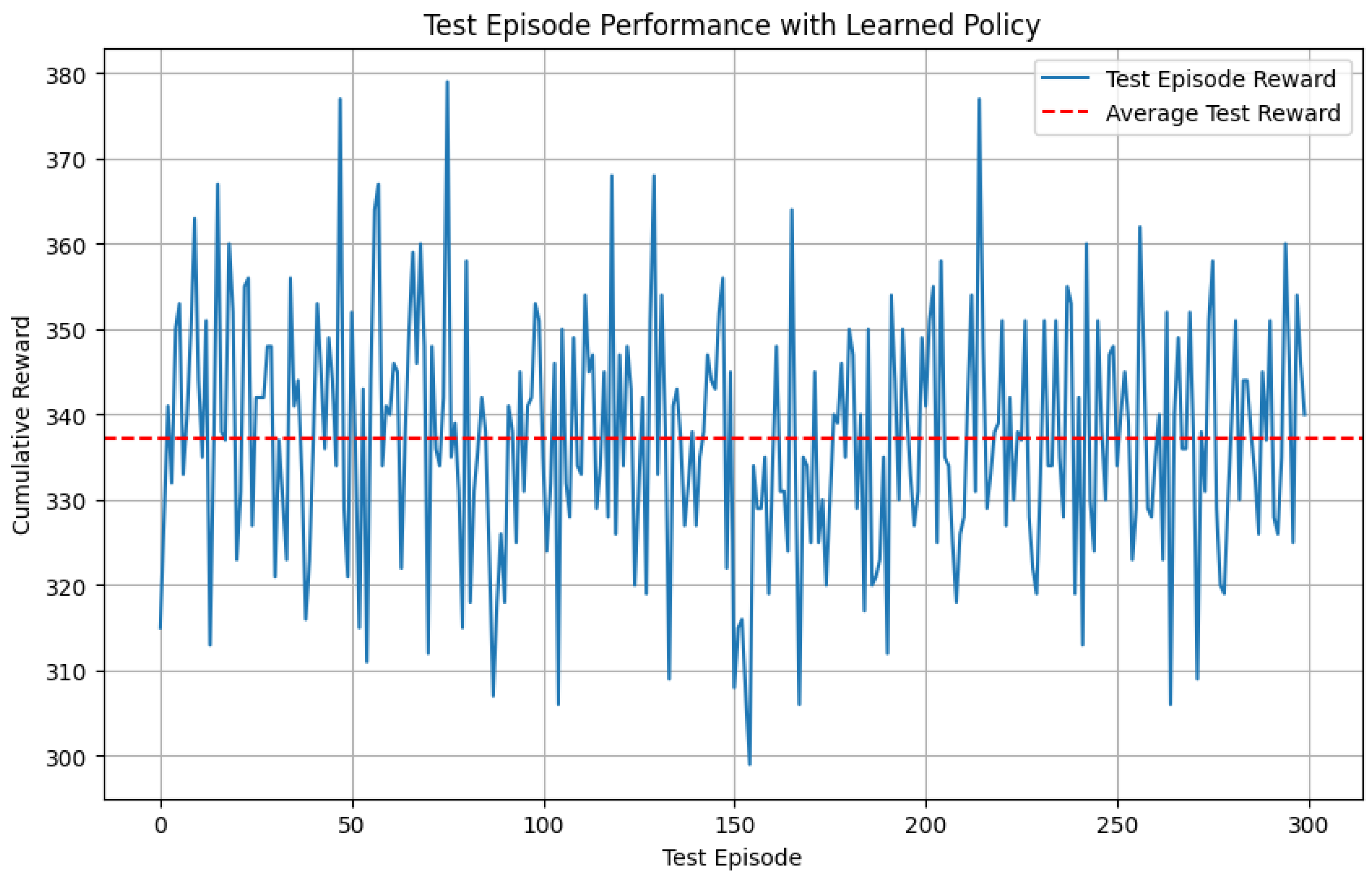
After deriving the optimal policy, we tested the trained model on 300 episodes to evaluate its performance when deployed. Figure 5 visualizes the cumulative rewards on 300 test episodes when applying the Q-learning policy. The blue line represents the reward obtained by following the Q-learning policy, while the red line represents the policy’s mean performance across the 300 test episodes, with a mean of 337.23.

Q-learning demonstrated exemplary performance in both training (330) and testing (337.23), indicating that an optimal policy will be achieved for unseen data and that the model has learned a sound decision-making strategy. This performance provides additional evidence of why Q-learning policy is well-suited for intrusion detection in network security. While the majority of IR mechanisms nowadays rely on familiar patterns and experience to respond to the influential cases in the environment, the current method is not only robust but also fast and adaptive, capable of handling unseen traffic and providing an adequate response.

4.7. Q-Learning Policy vs. Random Policy

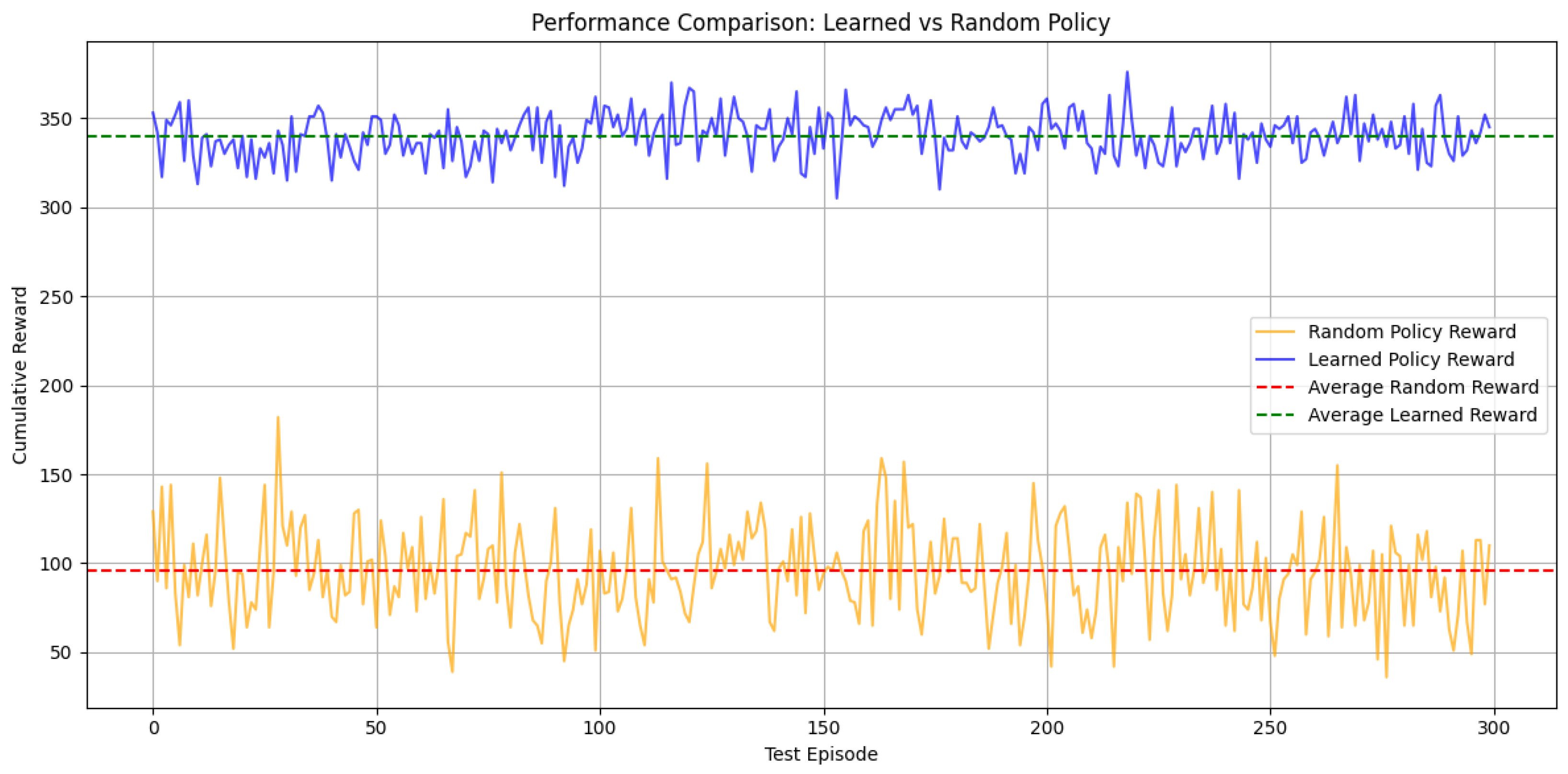
We compared the performance of the Q-learning policy with that of a random policy over 300 test episodes. The orange line represents the random policy reward, the red line represents the average reward of the random policy, and the blue line represents the Q-learning policy. Figure 6 illustrates that the random policy reward exhibits a high fluctuation rate and performs significantly worse than the Q-learning policy.

As shown in

Table 4. Comparison of Q-learning policy vs. random policy performance.

Policy	Average Cumulative Reward
Q-learning Policy (Learned)	330
Random Policy	95.55

, the Q-learning reward (330) is significantly higher than the random policy reward (95.55). This signifies that the Q-learning policy performs better than the random policy and emphasizes that random decisions yield inconsistent results. Learning from past experiences is essential in reinforcement learning.

The Q-learning policy not only yields a significantly higher average reward but is also far more stable (with lower variance) than the random policy. This implies that our agent selects actions in a way that is consistent with fewer deviations and, consequently, much higher rewards.

Figure 7 illustrates that the Q-learning policy has a much higher median, compared to the random policy, which also has outliers with observable skewness. Therefore, we can state that the Q-learning policy is more consistent, robust and ultimately achieves significantly higher performance.

4.8. Model Evaluation

We can use the estimated transition probabilities to determine how effectively our Q-learning agent performs. For that purpose, we need to find a solution to the MDP with our knowledge of the environment. Since our Q-learning algorithm does not use any transitional probabilities, it will be very beneficial to perform a goodness of fit analysis of the model. The transitional probabilities can be estimated only if we possess more knowledge about the environment. We could perform two methods to estimate them. The first method is if we know the distribution of the transitional probabilities and to generate transitions from that distribution, the other method is if we obtain them with an actual data set. For that purpose, we will use the NSL-KDD data set. The data set is provided by the Canadian Institute for Cybersecurity, at University of New Brunswick. In the last approach selected by us, we can evaluate our model by comparing the value $V\left(s\right)$, which we calculated with the Q-learning approach, with the value $V\left(s\right)$, which we will obtain by solving the MDP, knowing the transition probabilities.

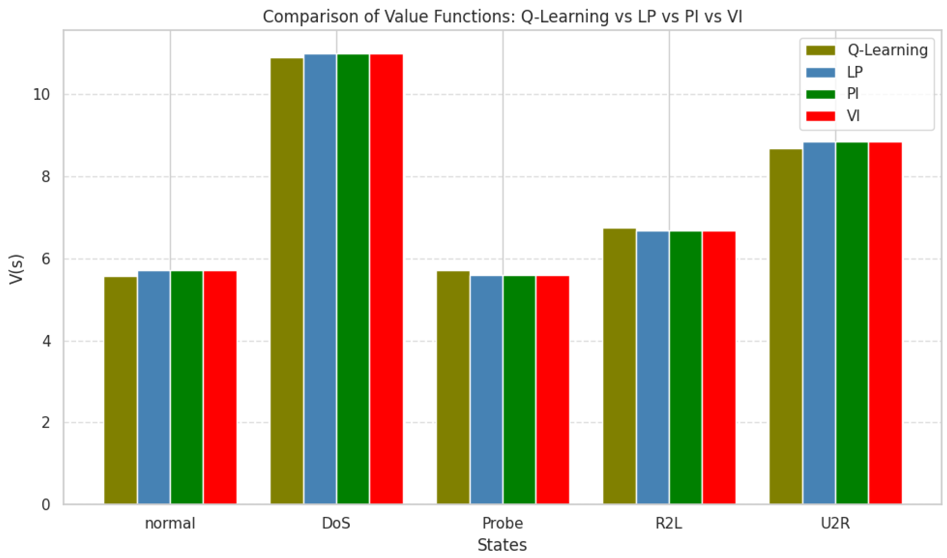
The aim is to create a root mean square error (RMSE), so we can test the effectiveness of the Q-learning approach. There are several methods, including linear programming (LP), policy iteration (PI), and value iteration (VI). All these solutions require knowledge of the environment, represented by the known transition probabilities. As shown in

Table 5. RMSE for Q-learning evaluation.

Method	${\mathbf{V}}^{*}\left({\mathbf{s}}_{\mathbf{Normal}}\right)$	${\mathbf{V}}^{*}\left({\mathbf{s}}_{\mathbf{DoS}}\right)$	${\mathbf{V}}^{*}\left({\mathbf{s}}_{\mathbf{Probe}}\right)$	${\mathbf{V}}^{*}\left({\mathbf{s}}_{\mathbf{R}2\mathbf{L}}\right)$	${\mathbf{V}}^{*}\left({\mathbf{s}}_{\mathbf{U}2\mathbf{R}}\right)$	RMSE
LP	5.716966	10.998375	5.592969	6.67405	8.847963	0.127007
PI	5.716966	10.998375	5.592969	6.67405	8.847963	0.127007
VI	5.716965	10.998374	5.592969	6.67405	8.847963	0.127006

and Figure 8, we can observe the RMSE errors using the results for $V\left(s\right)$ from Q-learning. The RMSE is calculated as follows:

$$\mathrm{RMSE}=\sqrt{{\displaystyle \frac{1}{N}}\sum _s{\left[V\left(s\right)-V^{*}\left(s\right)\right]}^2}$$

(6)

The Q-learning agent obtained the same $V\left(S\right)$ values for each state, regardless of the method employed to calculate these values. Value iteration, linear programming and policy iterations are methods applied to solve the Bellman equations regarding the estimated transitional probabilities. The obtained root mean square value is small, which signifies again the robustness and the efficiency of the model. When we protect our system, the response that the IR can provide must be independent of the knowledge of the transitional probabilities. In real life, those distributions are constantly changing, and if we apply an algorithm which is model-based or requires us to estimate the probabilities, then our agent may end up not being very useful, we would like to make sure the algorithm that we use is free from assumptions and to be effective in changing environment. The overall comparison performance is summarized in Figure 8.

4.9. Deploying the Policy on the NSL-KDD Dataset

After training the Q-learning agent, the learned policy was applied to the NSL-KDD dataset. We employed a feature reduction technique, utilizing only the features relevant to the dataset. In our case, we used gain ratio for ranking the features, based on their information gain. For each sample, the agent selected an action of whether to allow or block the traffic. The cumulative reward, accuracy, and confusion matrix were also computed to show how well the policy generalized to the dataset, reflecting the agent’s ability to response to intrusions effectively. The following results were obtained.

Table 6. Q-Table for Q-learning policy deployed on NSL-KDD dataset.

State	Allow (0)	Report (1)	Return (2)	Block (3)
Normal (0)	6.08946832	0.65195162	1.41350597	0.06186645
DoS (1)	−3.91069429	4.11094152	1.11089763	11.11111108
Probe (2)	0.00000000	0.00000000	0.00000000	0.00000000
R2L (3)	0.00000000	0.00000000	0.00000000	0.00000000
U2R (4)	0.00000000	0.00000000	0.00000000	0.00000000

above displays the result of the trained policy on the NSL-KDD Dataset. The Q-values suggest that the agent assigned zero values in the probe, R2L, and U2R states, indicating it did not encounter enough feedback or samples to update its Q-values. The data set is unbalanced, where attack samples dominate, and the agent did not experience enough normal traffic or other attack types. For the normal state, the agent learned that blocking or reporting a DoS attack results in positive rewards. Specifically, the Q-value of 11.11111111 for the “Block” action indicates that blocking a DoS attack is considered the most rewarding action. Similarly, the agent discovered that allowing traffic (Q-value of 6.10105437) was the best option in the normal state. The agent effectively learned to prioritize blocking malicious activity and allowing normal traffic when it encountered Dos attacks. However, due to the dataset’s nature, it had limited experience with other types of attacks.

5. Discussions

With the obtained results, we provided proof that reinforcement learning can be successfully applied in the IR as a controlling mechanism so our networks can stay protected, depending on the current situation of our decision agent. The application of Q-learning as an intrusion response mechanism is novel, and more research is needed in that area. Based on the results obtained from a broader perspective, Q-learning is a significant tool because the decision agent does not need to know much information to find optimal results. The Q-learning agent learns as it goes and makes decisions based on the feedback it gets from the environment. The agent does not need to know the transition probabilities; the only information he needs is the beginning state of the decision agent. Therefore, this method can be successfully combined with the classical classification ML methods. This model is not an alternative to classification techniques but a complementary instrument. The main idea is for the agent to receive initial information from the classification method so that it knows the beginning state. The proposed mechanism for intrusion response is unique and valuable. The Q-learning algorithm for IR is an excellent tool for an automatic response; there are ways to adapt to streaming data whenever the intrusion detection allows for streaming data classification set-up. This application could turn the Q-learning algorithm and transform the model into a powerful tool in modern security systems. However, this algorithm can be successfully implemented as it is. The first step is to extract the network traffic from the transmission control protocols and send it to the intrusion detection module, where the preferred classification method is applied; see Figure 9. The next step is to let the healthy traffic into the system and isolate the malicious traffic under quarantine. Then we could apply another classification tool that may classify the network as under “Normal”, “DoS”, “Probe”, “R2L”, and “U2R ”. After that classification, it is time for the Q-learning agent to observe the state that it is currently in and to select an optimal policy, based on the Q-learning algorithm. The reward–penalty system gives administrators a powerful mechanism to mitigate threats successfully and respond effectively to attacks. The proposed method can be further elaborated by adding more available information for the agent’s actions. Besides blocking and allowing the traffic in the system, we could add actions related to adjusting the security settings or going beyond protecting. The reward function could be further improved based on the cost function associated with the consequences of selecting a particular action. It is also possible to create a decision path for the agent just as we did in our proposed approach; however, when including more agents in the environment, some of them could be friends, neutral, or foes. Then, the agents will try to maximize their cooperative rewards and simultaneously achieve equilibrium points.

6. Conclusions

This paper demonstrated a noteworthy tool for the IRS and outlined the importance and necessity of creating novel, robust models and perspectives in the existing literature. We outlined the algorithmic structure of Q-learning from the perspective of a probabilistic model and proved its robustness. We simulated an MDP and created a decision agent whose decisions and actions depend on the environment’s interaction. We provided an example of a reward function so the agent can find an optimal policy and the action that maximizes its calue and action-value functions. The sensitivity analysis provides understanding of the decision nature of the agent, and the goodness of fit estimation demonstrates the soundness and efficiency of the model. The main advantage of the Q-learning model over current algorithms used in IR systems is the existence of a decision entity that can operate independently in a completely unknown environment and provide an automated response to malicious activities. The agent does not need to know any previous information about the network, and it learns fast with minimal assumptions based on the Markov Decision Process. Our future work is related to making the model more realistic regarding the reward function; we need to create an updatable reward mechanism that depends on the cost function of the decision agent and other factors of the security environment that are changing over time. Including more agents who may work in a competitive or cooperative network setup will be very beneficial. This approach will provide more insights about the entity “attacker” and model its behavior sophisticatedly so a game theory aspect of the environment can be applied. We also need to create a grid search mechanism to tune the parameters more appropriately and to create advanced performance metrics, besides MSE, that will serve as an evaluation tool and be reported at any time in the IR systems. Many new deep Q-learning approaches would also benefit our decision agent, and they need to be explored further in our analysis. Our goal for this paper is to provide a complete outline of the probabilistic structure and application of the model to network security, and our future work will be devoted to researching the individual components and steps of the Q-learning algorithm in a deeper context so that the overall model can be further improved and efficiently serve society.