AI-Based Impact Location in Structural Health Monitoring for Aerospace Application Evaluation Using Explainable Artificial Intelligence Techniques

Abstract

Due to the nature of composites, the ability to accurately locate low-energy impacts on structures is crucial for Structural Health Monitoring (SHM) in the aerospace sector. For this purpose, several techniques have been developed in the past, and, among them, Artificial Intelligence (AI) has demonstrated promising results with high performance. The non-linear behavior of AI-based solutions has made them able to withstand scenarios where complex structures and different impact configurations have been introduced, making accurate location predictions. However, the black-box nature of AI poses a challenge in the aerospace field, where reliability, trustworthiness, and validation capability are paramount. To overcome this problem, Explainable Artificial Intelligence (XAI) techniques emerge as a solution, enhancing model transparency, trust, and validation. This research presents a case study: a previously trained Impact-Locator-AI model is, initially, demonstrating a promising location accuracy; however, its behavior in real-life scenarios is unknown, and before embedding it in an aerospace structure as an SHM system its reliability must be tested. By applying XAI methodologies, the Impact-Locator-AI model can be critically evaluated to assess its reliability and potential suitability for aerospace applications, while also laying the groundwork for future research at the intersection of XAI and impact location in SHM.

1. Introduction

In today’s aerospace industry, composite structures represent a very significant percentage of the mass of aerospace vehicles. Although their use is widespread and their stiffness-to-mass ratio is superior to metallic materials such as aluminum or steel, there is one characteristic that invalidates their use in some applications: they have no plasticity. Low-energy impacts (under 5 J) [1] can cause various types of damage, such as cracks in the polymer matrix, fiber fractures, or delamination [2]. This represents a big issue because, even if a notorious delamination will appear on the opposite side of the impact, the lack of indentation will mean that a visual external examination will not locate obvious damage. This means that for these structures an exhaustive (and expensive) non-destructive inspection must be performed in order to ensure safe operation along the whole lifespan of the vehicles [3,4,5,6,7,8]. This is why Structural Health Monitoring (SHM) was created [9,10,11]: to assess the integrity of structures using sensors and data analysis.

Impact localization has been analytically performed using triangulation based on the Time of Arrival (ToA). However, ToA-based triangulation requires knowledge of the propagation velocity of the Lamb waves generated by the impact [12,13]. In composite materials, this velocity varies depending on the stacking sequence at each point of the structure. Furthermore, Lamb waves decompose into symmetric and antisymmetric modes. The symmetric mode (associated with the change of thickness) propagates faster but has a lower amplitude, often making it indistinguishable from sensor noise. In contrast, the antisymmetric mode (associated with structural bending) exhibits a slower propagation velocity. However, its detection is complicated by the prior arrival of the symmetric mode, which interferes with the onset identification of the impact event. Furthermore, the propagation velocities of Lamb waves also depend on the thickness of the medium, which further complicates the definition of the ToA of an impact.

Artificial Intelligence (AI) models can address a higher performance at the time of locating an impact because of their non-linear behavior. The applicability of this technology (AI) to the SHM field has been proved in aerospace [14]. In particular, AI has demonstrated remarkable performance in accurately locating impact events, even when applied across diverse SHM technologies such as Piezoelectric (PTZ) sensors [15,16,17,18,19,20,21] and Fiber Bragg Gratings (FBGs) [22,23] by effectively analyzing the corresponding recorded vibration signals.

Nevertheless, even if the performance of an AI model during testing appears impressive, this does not necessarily imply that the model is functioning reliably or generalizing effectively in practical scenarios. Although a model that performs poorly can be definitively shown to be ineffective, it is not always possible to assert with complete certainty that a model is performing well. This is why AI models must be evaluated from multiple points of view to try to detect flaws in their reasoning. Explainable Artificial Intelligence (XAI) methodologies are techniques that enable the evaluation of AI models in a manner that is more interpretable and understandable from a human perspective. This methodology has already been used in the past [24,25,26] in order to understand the decision-making process of AI systems for different damage identification scenarios (but never in impact location applications) by applying XAI methodologies as Local Interpretable Model-Agnostic Explanations (LIME) [27] or Shapley Additive Explanations (SHAP) [28] to a specific prediction interpretation.

This current work presents a case study as a paradigm of the current situation of AI-based SHM systems: an SHM-AI model is, initially, showing promising results, but a higher level of reliability is required. By applying XAI methodologies, this reliability can be assessed and then its potential suitability for certain applications.

In this case, a Deep Neural Network (DNN) model was previously trained to predict impact locations in a stiffened flat composite structure [29]. PTZ sensors were embedded in a test plate and were used as receptors (passive function) to record impact vibrations. These impacts were performed with an autonomous CNC impactor machine. With the recordings of these impact vibrations, a wide and varied dataset of different impacts was created and, with it, a DNN model was trained. Even though the results of this model are promising (around 3.5 mm of mean error in a 752.3 mm square plate), its behavior in real-life scenarios is unknown because the decisions taken at the time of making a prediction cannot be understood in human terms. So, before embedding it in an aerospace structure as an SHM system, its reliability must be enhanced through a deeper analysis.

Now, with the present work, existing XAI methodologies based on LIME [27,30,31] have been studied and modified to adapt them to the situation described before. The idea is to examine the previously trained Impact-Locator-AI model behavior when dealing with multi-channel time-series data, especially considering that the trained model is a DNN rather than a Convolutional Neural Network (CNN) or a Recurrent Neural Network (RNN), in which the interrelation between channels is inherent to their own architecture. The adaptation of these pre-existing methodologies to the problem is focused on generating a human-readable explanation of how the model is taking into account different sensor’s signals to make predictions and which signal features are more relevant for the final decision. In doing so, this work not only supports a more transparent evaluation of the model’s internal reasoning but also contributes to laying the foundation for further research into explainable impact-location systems for SHM applications.

2. Materials and Methods

As was previously pointed out, the creation of the dataset and the design, training, and evaluation of the model’s performance was previously described in [29]. However, a brief insight into these aspects is given below.

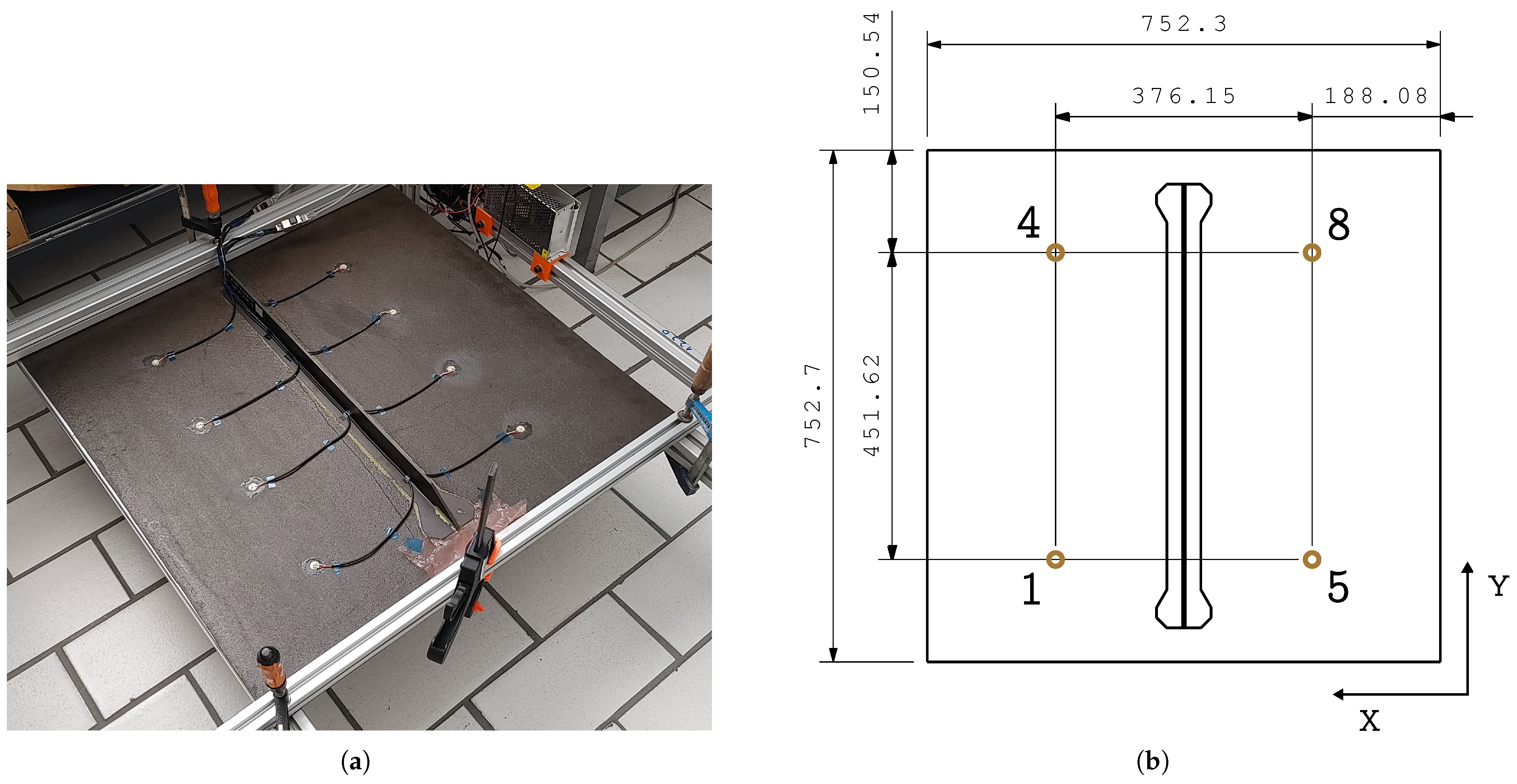
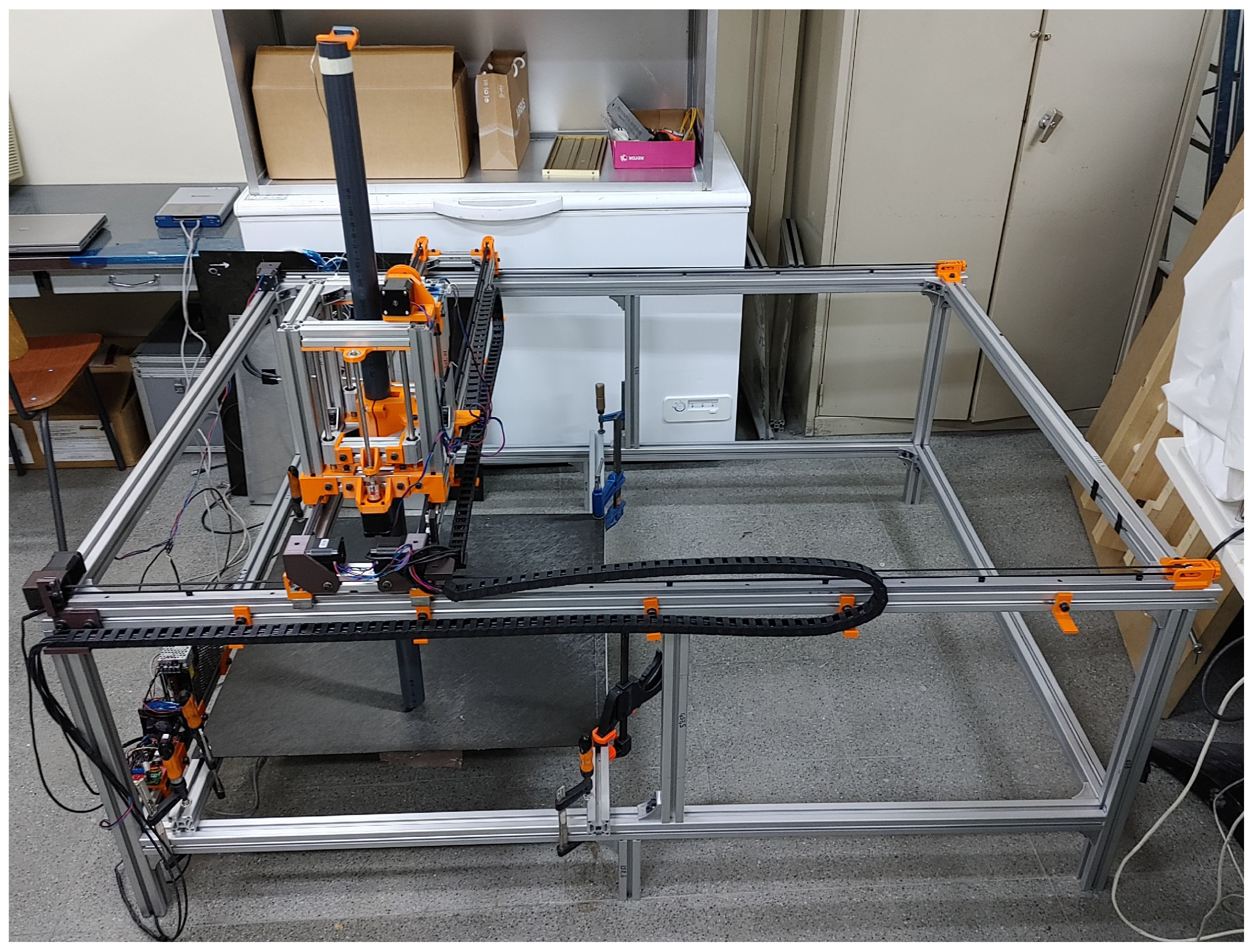
2.1. Specimen, Impactor, and Dataset

The impacted specimen is a 752.3 × 752.7 × 2 mm³ Carbon Fiber-Reinforced Plastic (CFRP) panel composed of a quasi-isotropic stacking sequence of a unidirectional prepreg with a T-beam stiffener, which can be seen in Figure 1a. A detailed description of the geometry is provided in Figure 1b, where 20 mm diameter 7BB-20-3 PTZ sensors are also located.

Signals from these sensors are recorded using a National Instruments NI-USB-6356 data acquisition card with a sampling rate of 125 kHz. This acquisition card is synchronized with a CNC-based Autonomous Impact Machine (see Figure 2) which autonomously performs the database generation. The impacted grid (15 × 17) and boundary conditions are shown in Figure 3. At each point of the grid, impacts were performed with a different combination of 5 masses (from 60 to 260 g with 50 g spacing) and 10 velocities (corresponding to a free fall from heights from 35 to 260 mm with 25 mm spacing) and repeated 5 times per combination. Before training the models, a process of detection of poorly recorded impacts is carried out and they are eliminated from the database, ending with almost 35,000 impacts.

The signals of the impacts and coordinates are normalized with the minimum and maximum values of each training group to avoid data leakage between sets. For this study, only sensors 1, 4, 5, and 8 have been used because of the coupling between sensors detected in del Rio et al. [29].

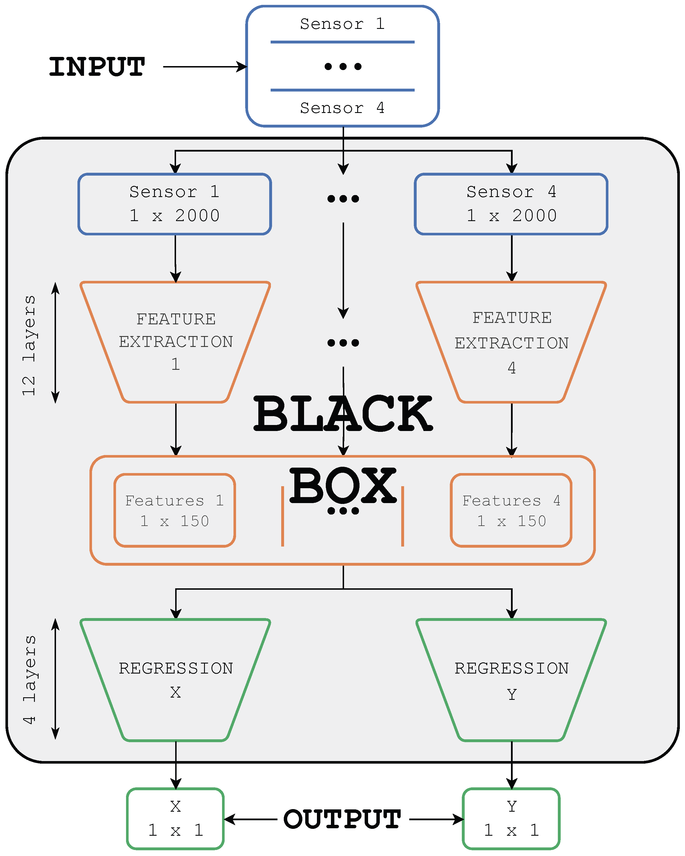
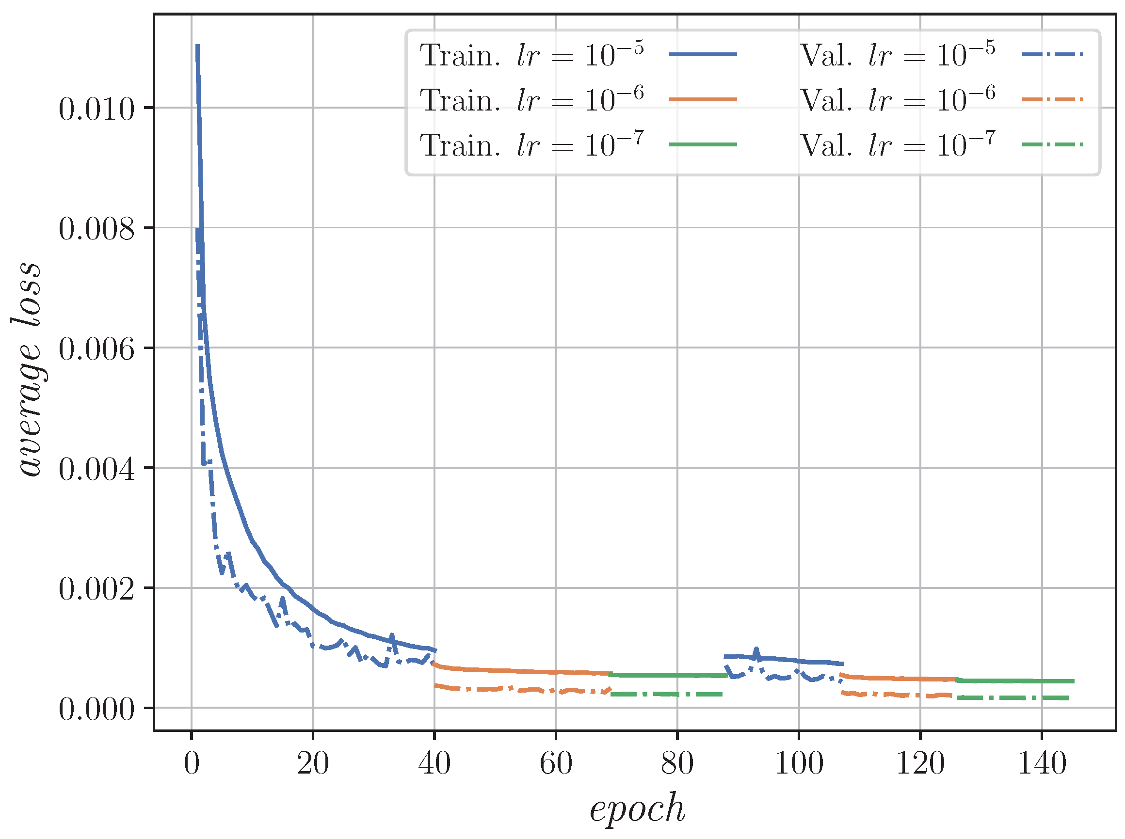
2.2. Impact-Locator-AI Model Evaluated

The model evaluated in this study has the same architecture defined in Figure 4, a detailed explanation of which can be found in del Rio et al. [29]. However, as long as the model will be evaluated as a black box through the chosen XAI methodology, only the input and the output are relevant. The input of the architecture is a 4 × 2000 array, corresponding to 4 time series of 2000 samples (16 ms as it was acquired at 125 kHz), and its output is a 1 × 2 array, corresponding to the X and Y coordinates.

The training process was performed with the training set, and the absence of overfitting was checked by analyzing the validation set behavior. Figure 5 shows that the loss of both sets drops with the iterations demonstrating that there is no overfitting in the training of the models.

To evaluate the performance of the model architecture, four random training, validation, and test distributions (k-Cross Validation with $k=4$) are generated. Once all models are trained, their performance is evaluated with the test set, and their results are collected in

Table 1. Performance metrics for the trained models. For more information, see [29].

Model [k]	$\mathit{\mu }\left(\mathit{EE}\right)$ [mm]	$\mathit{\sigma }\left(\mathit{EE}\right)$ [mm]
1	3.54	2.29
2	3.37	2.29
3	3.50	2.25
4	3.47	2.38
Average	3.47	2.30

(for a more detailed description and explanation, see [29]). For the following sections, Model 1 was selected.

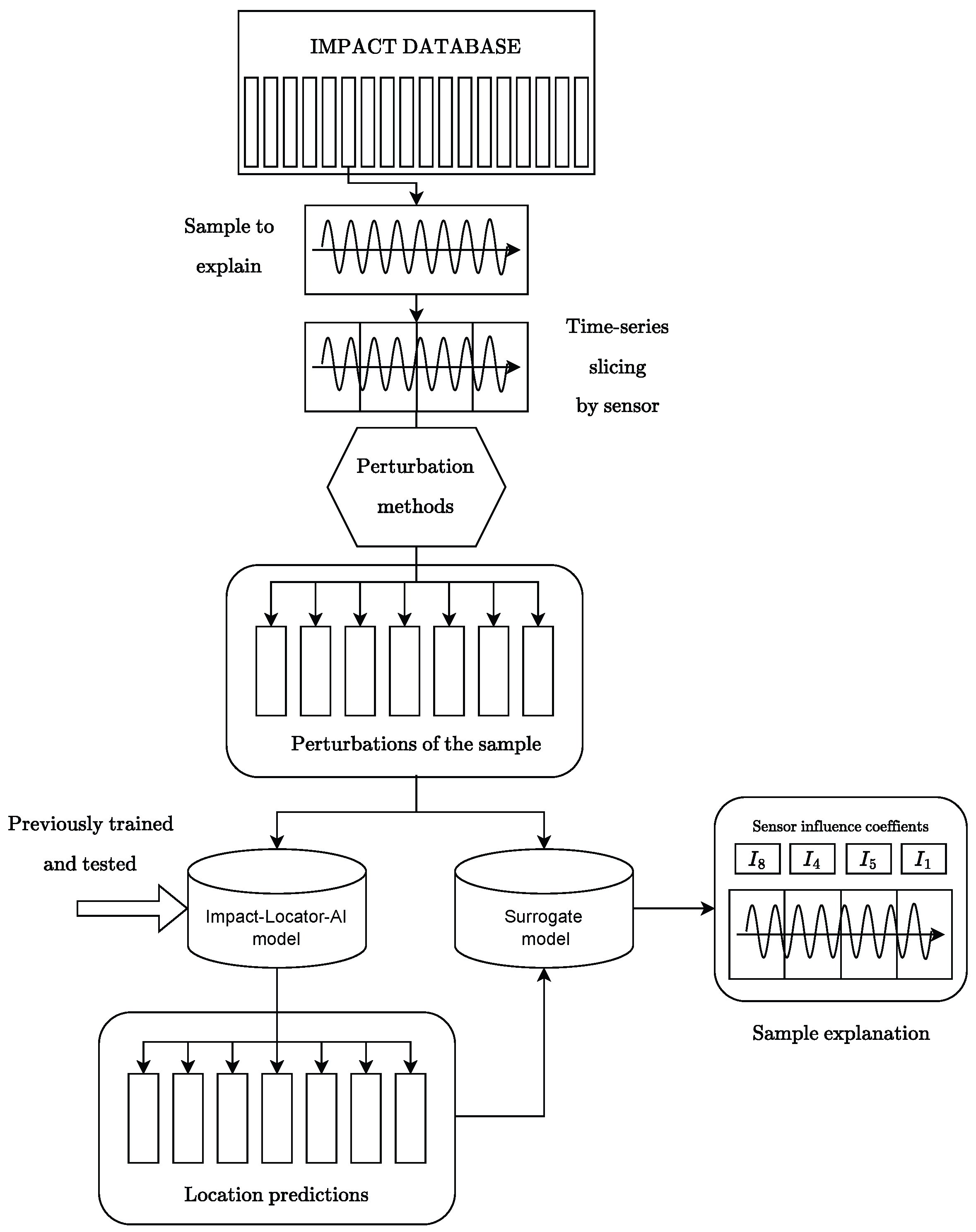
2.3. Explainable Artificial Intelligence

Among all available XAI methodologies, LIME (0.2.0.1) [27] was chosen because of its simplicity and versatility. The idea behind this technique is explaining predictions of complex black-box machine learning models using simpler, interpretable models.

To create this model, a sample of input data is perturbed, and the black-box model is fed with these data. Then, a surrogate model is fitted by comparing the variation in the output according to the proximity of the perturbed input with the original one. This surrogate model explains the behavior of the black-box model in the local region by regressing a coefficient of influence for each input element. The prediction can be linearly explained as the weighted sum of these input elements’ values times its influence coefficient.

This linear explanation is more accessible from a human interpretability standpoint because the influence of each input feature on the final prediction can be explained by a single coefficient. Once this explanation is obtained, the subsequent step is the interpretation of the results. This process requires domain expertise, as the evaluator must possess sufficient knowledge of the application area to assess whether the most influential features bear meaningful physical significance.

When analyzing time-series data, a critical challenge arises due to the high dimensionality of the input. Each sample point constitutes a feature, resulting in a volume of information that is, again, difficult to interpret. Moreover, isolated fluctuations in the signal often lack semantic relevance and may not convey meaningful information in human terms, particularly given the temporal dependencies among sample points. Consequently, a common strategy involves perturbing contiguous segments of the signal rather than individual sample values. By applying various perturbation techniques to these segments, it becomes possible to assess their influence on the black-box model’s predictions and, in turn, determine whether the model is capturing relevant temporal patterns or key features within the signal [30,31].

In the present work, the objective is to understand how the model interprets different sensor’s signals to predict the impact location. To elucidate this behavior, instead of perturbing arbitrary input segments, the full input is divided by sensors and then only one sensor’s signal is modified for each perturbation performed. Once enough perturbations have been performed, affecting different sensors, the Impact-Locator-AI model makes predictions out of this perturbed input and the influence can be retrieved by the surrogate model. A conceptual diagram of this algorithm is shown in Figure 6.

The perturbation methods specifically designed for this application alter each sensor’s signal individually in a manner that targets distinct and potentially relevant signal features; therefore, a subsequent interpretation can be performed. The perturbation methods applied are the following:

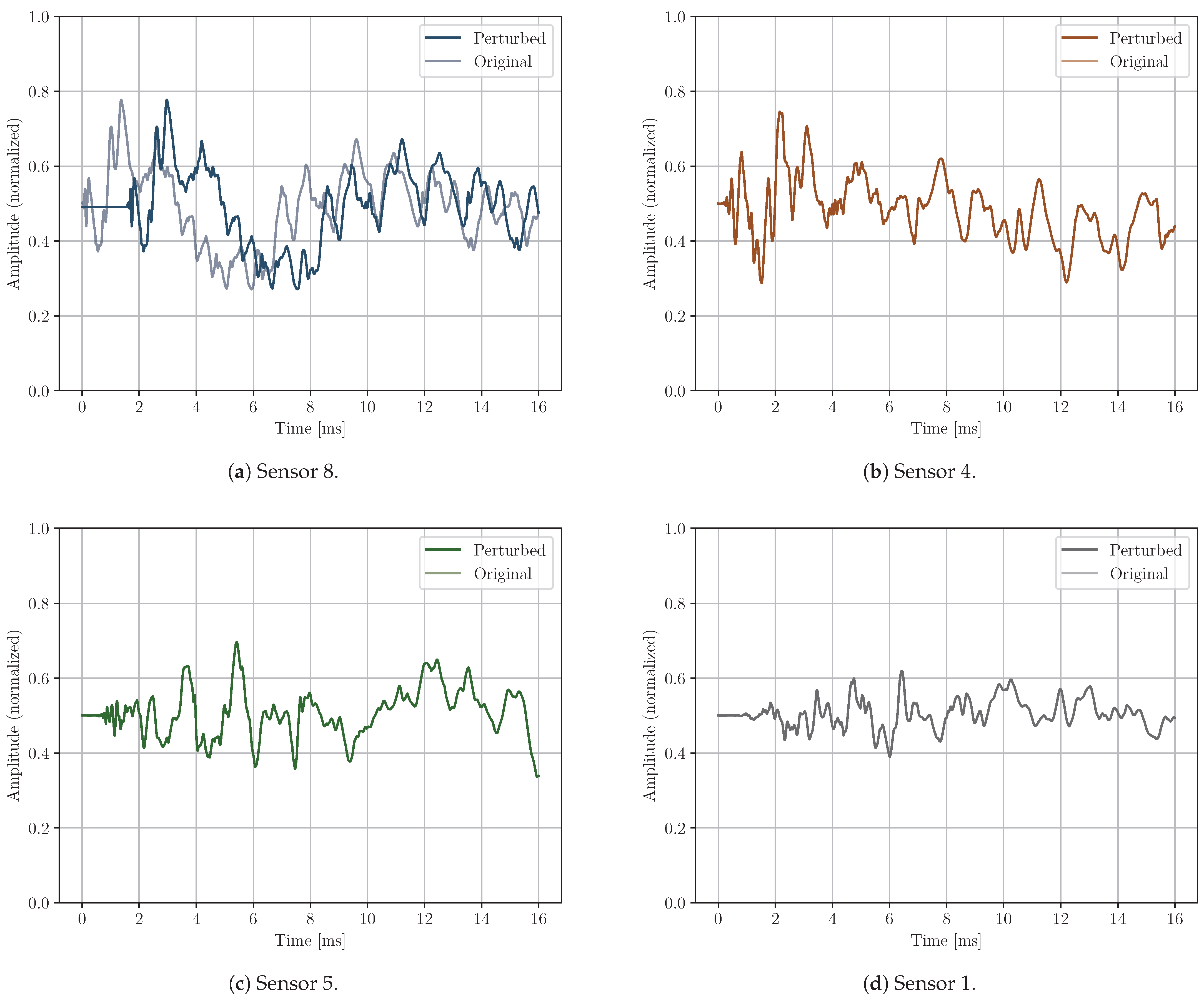
• Time delay: the signal is shifted and zeroes are appended to the beginning or the end of the signal (see Figure 7). This perturbation modifies the ToA of the signal of one sensor. From a practical standpoint, it simulates a displacement of the sensor relative to the position it occupied during the model’s training phase.
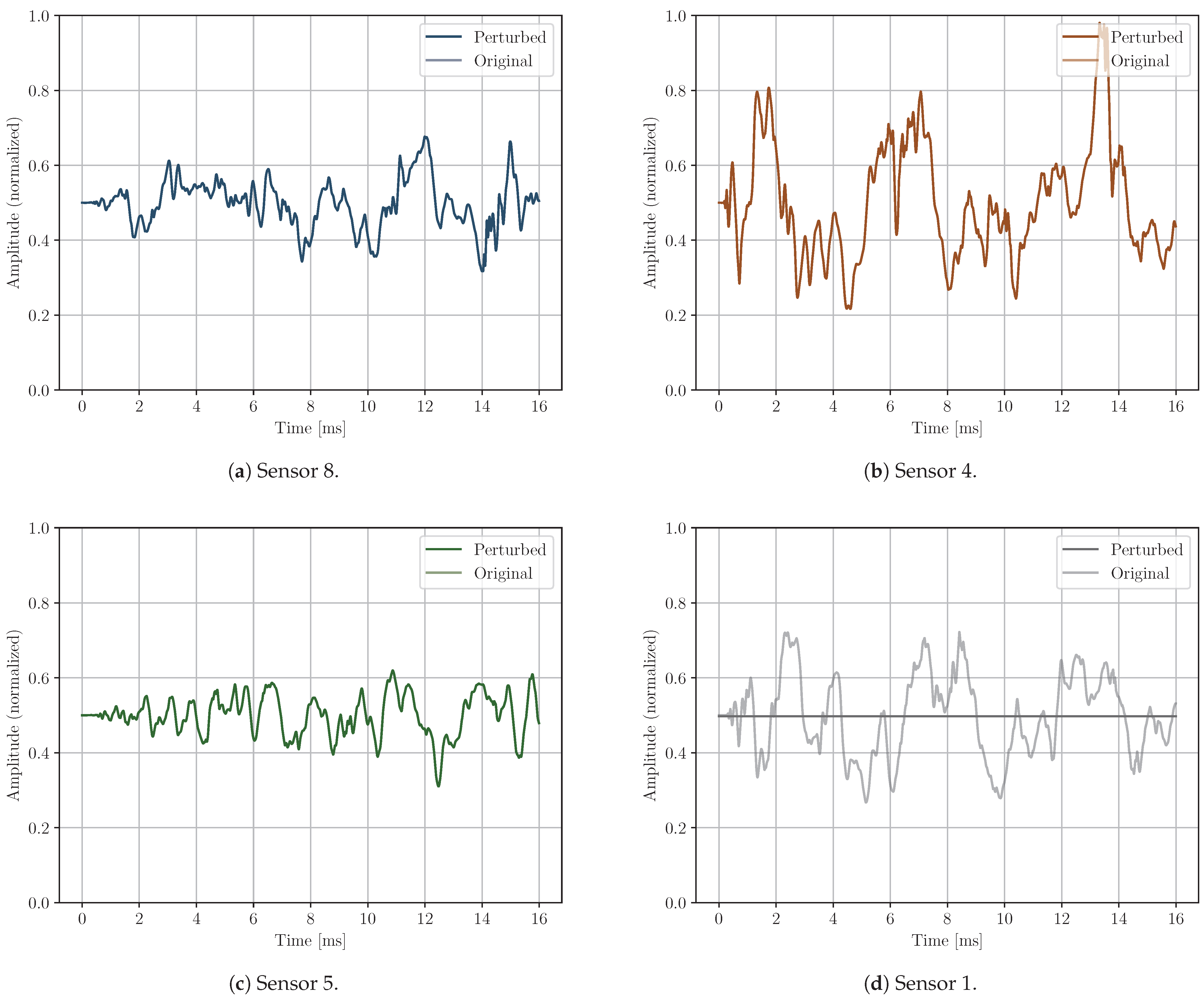
• Sensor cancelation: a sensor’s signal is substituted by its mean value as if it has no signal recorded (see Figure 8). This perturbation allows for the assessment of model performance in the absence of information from a specific sensor. From a practical standpoint, it simulates one sensor breakage during the operational life of the monitored aerostructure.
• Noise: white noise of a 0.1 signal-to-noise ratio (SNR) is applied to one of the sensor’s signal (see Figure 9 and Figure 10). This perturbation aims to evaluate the model’s capabilities when dealing with noise. From a practical standpoint, it simulates variation in external conditions.

As said before, out of the perturbed input data, the locator model (black box) will make predictions that will differ from the original unperturbed input data. In Figure 11, the Impact-Locator-AI model’s predictions from perturbed data are represented alongside the original prediction and the true location of the impact. This figure shows how the predictions of the perturbed samples have a very large error compared to the prediction of the unperturbed sample.

By applying the LIME-XAI technique to a single prediction, the influence (as a value) of each sensor on the final prediction can be retrieved. In Figure 12, the four sensors’ influence is plotted for different impact location explanations.

Even though this approach may be valid for understanding individual predictions, a different methodology must be adopted to preserve the interpretability of the explanation when assessing the overall behavior of the model across the entire impacted plate and from the perspective of the sensor. In order to visualize this behavior, a heatmap for each sensor is created where the value represented in each coordinate is the influence of this sensor for this location prediction. For each coordinate, more than one sample is available because impacts were performed with several masses and velocities. Because of that, not only is the mean value of each coordinate’s influence represented, but (in some cases) the standard deviation is also analyzed to understand how the model responds to these variables (mass and velocity), which must not disturb the location prediction. A conceptual diagram of the whole algorithm developed specifically for the problem studied is shown in Figure 13.

3. Results

In this section, different results obtained from different perturbation methods are shown. In each set of heatmaps, the upper and lower limits of the common color bar have been set. This makes it possible to identify the greater or lesser influence of each sensor on the final prediction.

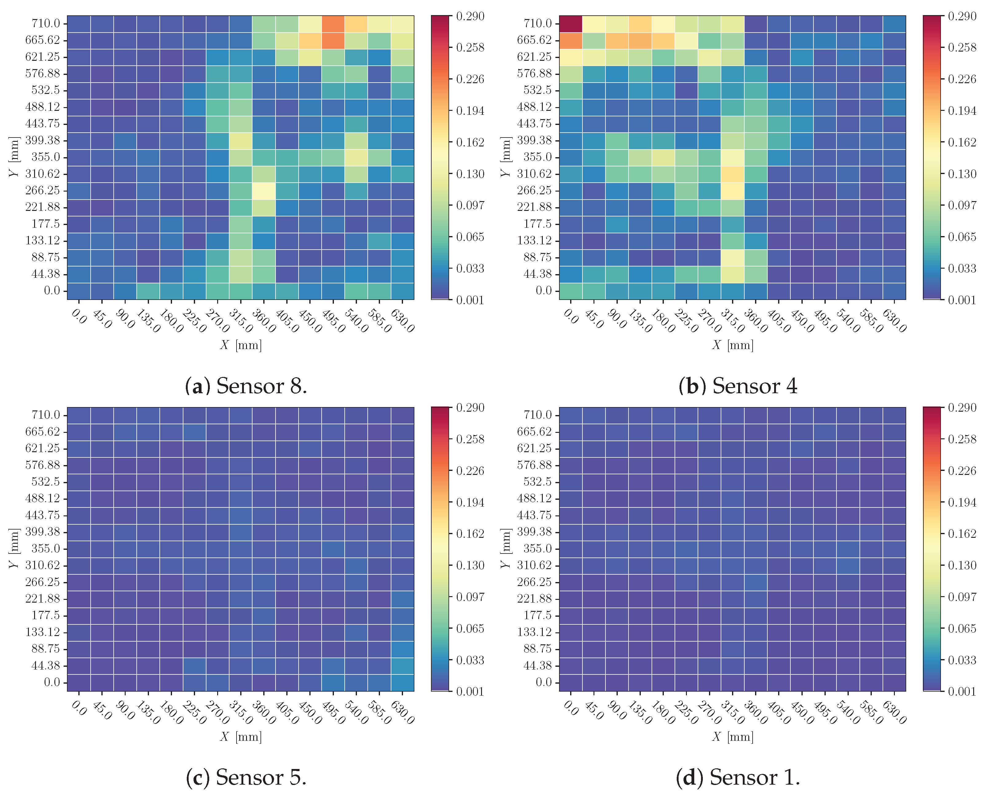
3.1. Time Delay

Heatmaps of time delay perturbation analysis are shown in Figure 14 and Figure 15 for $\pm 0.16$ ms (for X and Y predictions, respectively) and in Figure 16 and Figure 17 for $\pm 1.6$ (for X and Y predictions, respectively). In all of them, the mean value of the sensors’ influence for each coordinate’s different impacts is explained.

When a small time delay is induced in the sensors, it has no appreciable influence on the predictions, as shown in Figure 14 and Figure 15. When this delay is increased by 10 times (Figure 16 and Figure 17), its influence also increases from a maximum of ${10}^{-2}$ to 0.290. However, the influence of Sensor 1 is not affected by the increase in delay as it remains close to ${10}^{-2}$. Both X and Y coordinate predictions show similar behavior.

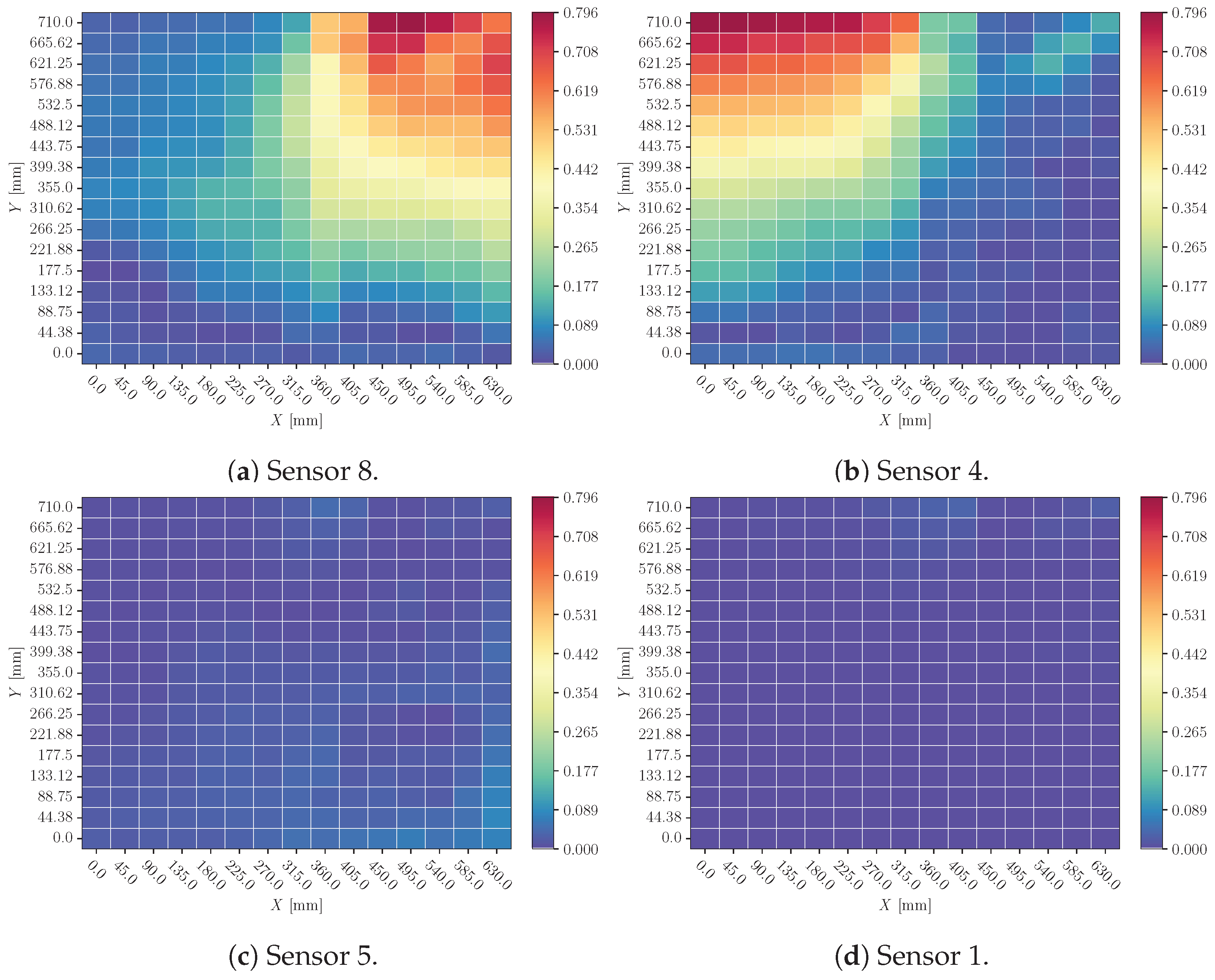
3.2. Sensor Cancelation

Heatmaps of sensor cancelation analysis are shown in Figure 18 and Figure 19 (for X and Y predictions, respectively) and also in Figure 20 and Figure 21 (for X and Y predictions, respectively). In the first two figures, the mean value of the sensors’ influence for each coordinate’s different impacts is explained, and the second two show the standard deviation. In this case, the influence of subtracting one sensor’s signal has a remarkable effect on the coordinate predicted.

For X-coordinate prediction, the influence of Sensors 8 and 5 is prominent for predictions made in their symmetrical position along the X direction, whereas Sensor 4 is more relevant for the whole opposite edge, and Sensor 1 has no influence at all. If combined, the main influence areas of Sensors 8, 4, and 5 cover almost the whole plate. The standard deviation of the influence (∼10⁻²) is reduced in comparison.

For Y-coordinate prediction, the behavior is different. In this case, Sensors 8 and 4 have the most relevant influence areas in their opposite corners along the X direction. If combined, the main influence areas of these two sensors are the upper part of the plate. Again, the standard deviation of the influence (∼10⁻¹) is reduced in comparison.

3.3. Noise

Heatmaps of 0.1 SNR white noise perturbation analysis are shown in Figure 22 and Figure 23 (for X and Y predictions, respectively). In all of them, the mean value of the sensor influence for each coordinate’s different impacts is explained.

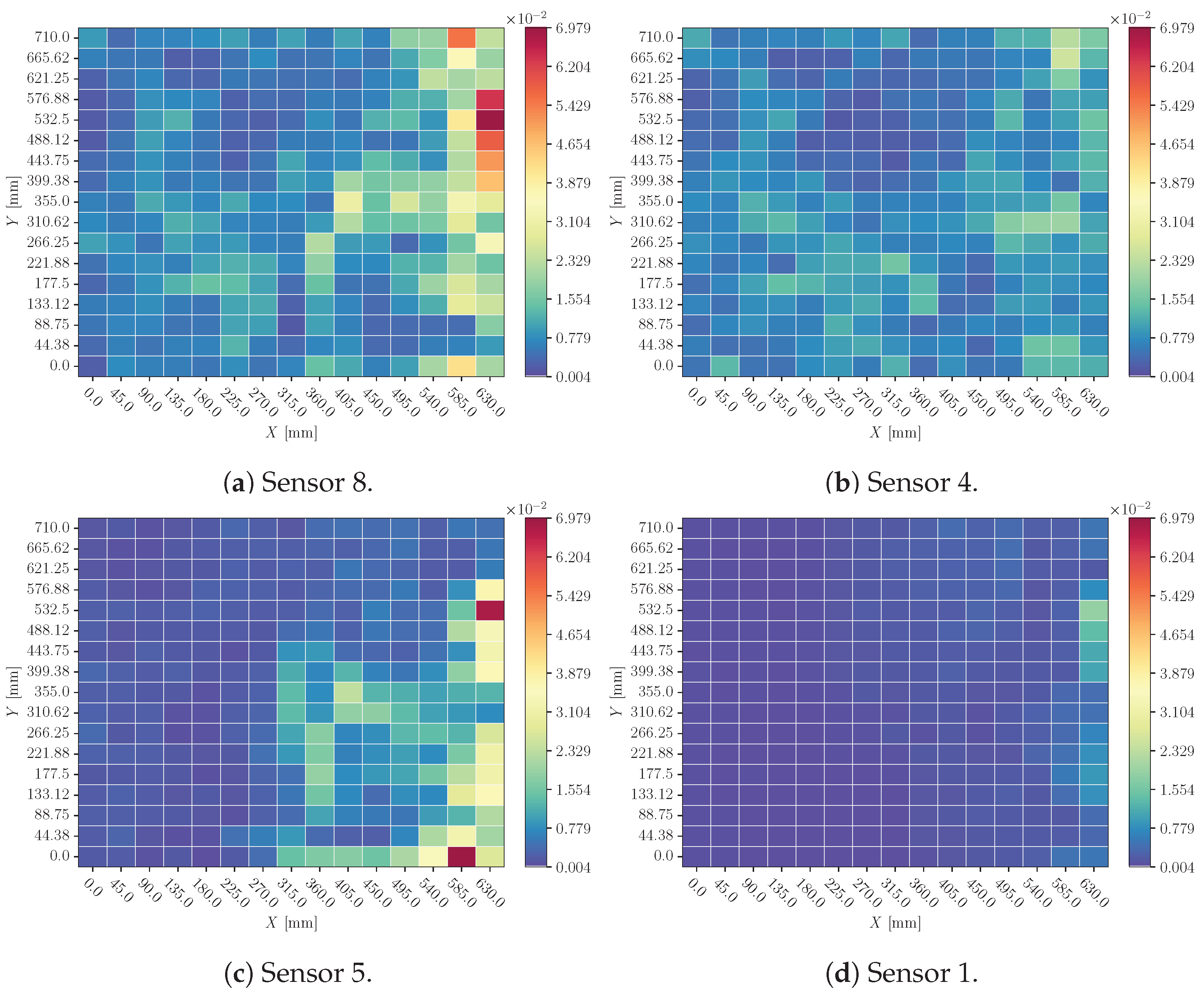
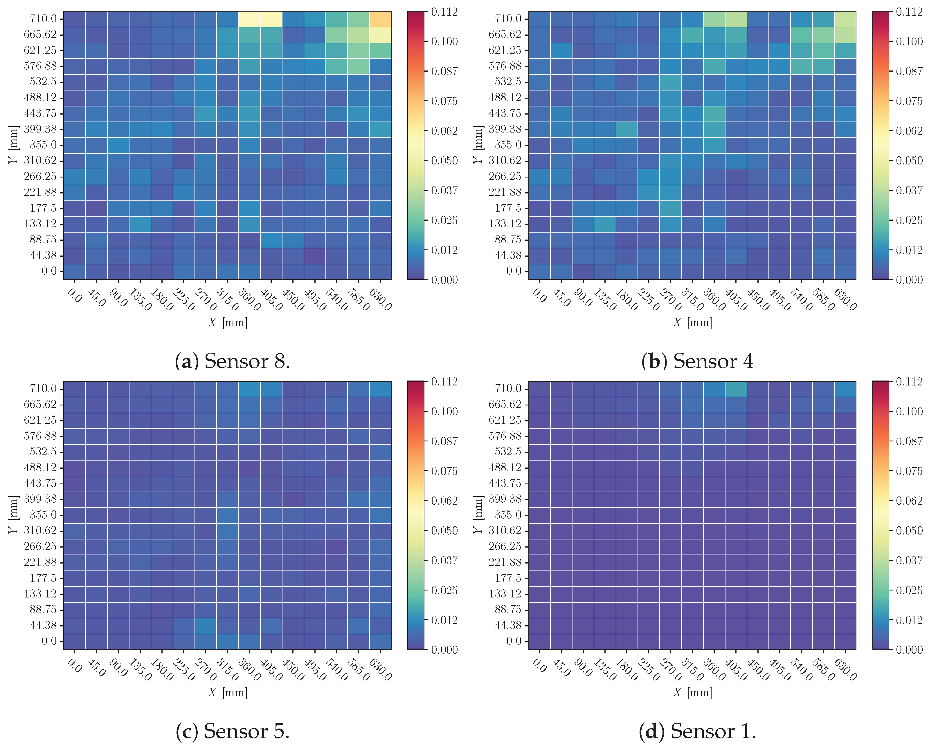
In this case, for both X and Y impact coordinate predictions, the influence of the noise perturbation is reduced (∼10⁻⁴) for all the sensors with some random and small variations over the whole plate. It is remarkable that the impacts performed in the farther edges of the origin (corresponding to each coordinate) have even less noise influence.

4. Discussion

4.1. Time Delay

When a time delay is introduced into sensor signals, there is not a significant variation in the prediction (Figure 14 and Figure 15), but if the perturbation range is wider (Figure 16 and Figure 17), the behavior is consistent: values of influence are higher and the distribution is similar.

From these results, we can conclude that Sensor 1 has virtually no influence on the model’s final prediction and that the signal’s ToA has little influence on localization. This suggests that the model utilizes the relationships between the signal’s maxima and minima when it has a larger amplitude.

4.2. Sensor Cancelation

When a sensor’s signal is replaced by its mean value (Figure 18 and Figure 19), there is a substantial perturbation in the predictions. Again, Sensor 1 seems to be discarded by the model: its influence is reduced in comparison with other sensors.

Also, perturbations around impacts with different mass and velocity configurations do not have a huge dispersion (Figure 20 and Figure 21). This suggests that the model is not considering these magnitudes’ influence on the signal, and it distinguishes only the effects related to impact location.

These results are in line with the fact that to locate an impact by triangulation, the minimum number of sensors is three.

It is also remarkable that the behavior between X and Y prediction is slightly different, but considering the stiffener and the different boundary conditions, this variation is understandable.

4.3. Noise

When a sensor’s signal is perturbed with white noise (Figure 22 and Figure 23), the influence of the perturbed sensor is negligible. Heatmaps show homogeneous values over the whole plate, and only some random points are slightly highlighted; additionally, no sensor is more affected than the others. Therefore, the model is filtering the signal prior to making the prediction. The fact that the model filters the signal also shows that the most representative Lamb wave mode is anti-symmetric (bending) as the symmetric mode would be masked by the noise itself, and filtering it out would remove it.

5. Conclusions

Out of the present work, the following conclusions about the Impact-Locator-AI model can be drawn:

• Even though time delay must be the most relevant perturbation at the time of making a prediction, the model is not highly affected by this effect. This leads to the conclusion that the model compares different sensor signals to make a more robust prediction relating the Times of Arrival between sensors. When different time delay ranges of perturbation are studied, the model seems to have a consistent response, which is a desirable characteristic.
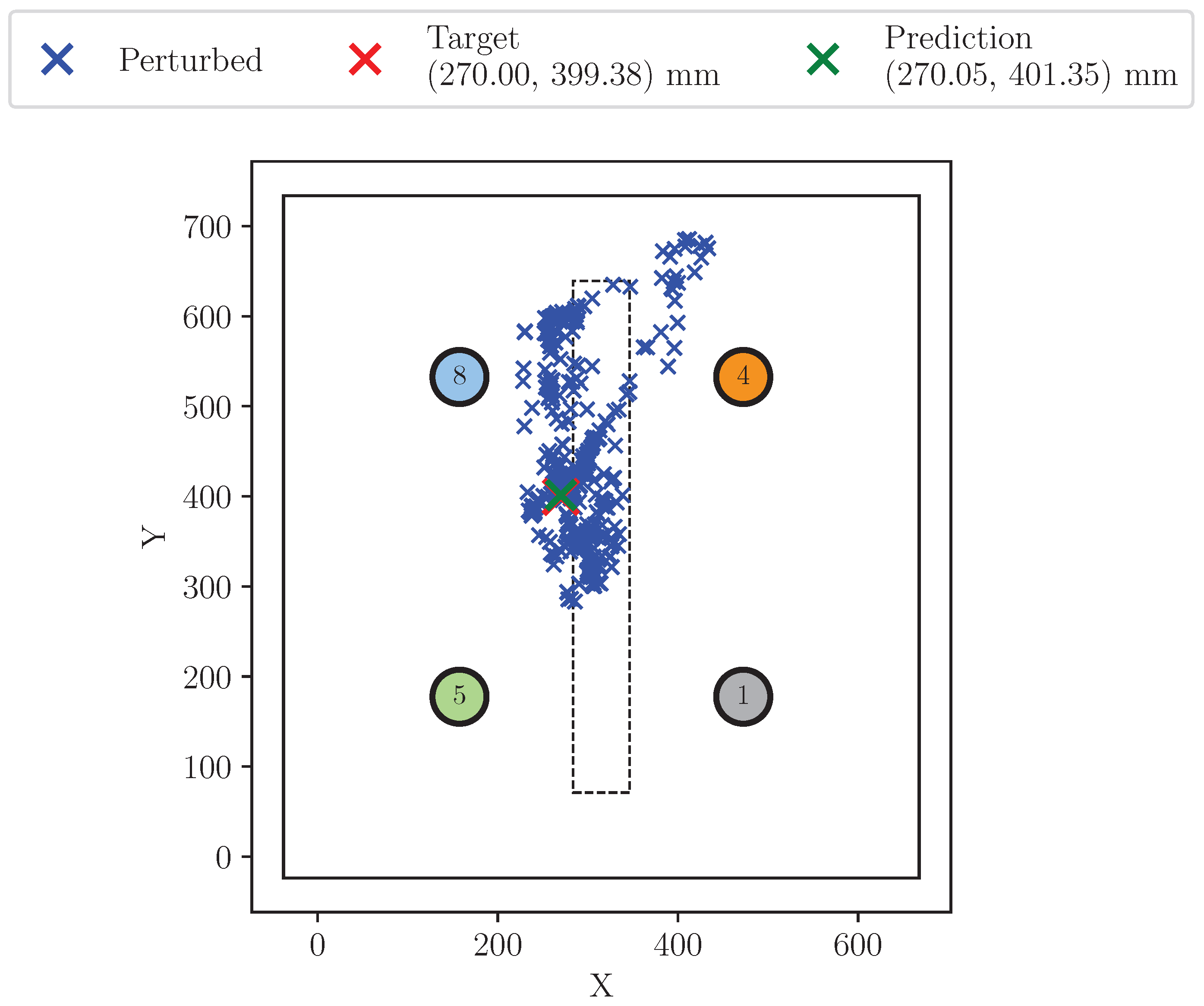
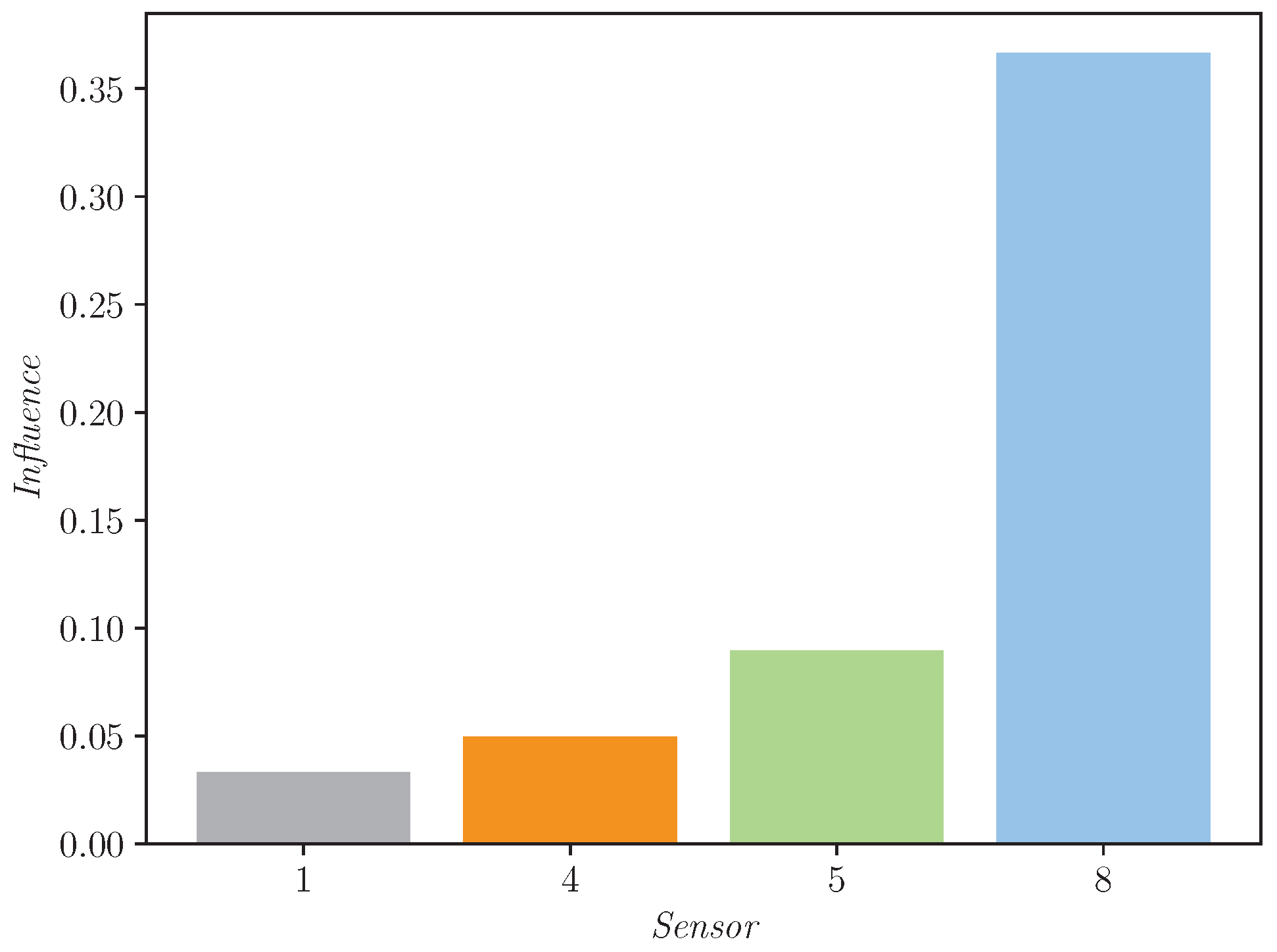
• When a sensor’s signal is canceled, the influence is significant. This behavior is consistent with the time-delay results. Due to the lack of a signal, the relationship between sensors cannot be properly obtained, and the model prediction is highly influenced.
• Noise perturbation has no remarkable influence over the sensors, and no sensor is especially more affected. This means that the model is filtering the signal prior to making the prediction, which is a valuable characteristic if the SHM system is embedded in an aeronautical structure.
• Mass and velocity have no influence on the locator model when the perturbations are performed, which means that the model is able to understand the signal correctly.
• Sensor 0 perturbations do not have a major influence on the final decision. This means that the model is discarding it, which is absolutely logical considering that only three sensors are needed to triangulate a position.
• The two values predicted by the model (X and Y impact coordinates) have a slightly different behavior. This can be related to the stiffener presence and the different boundary conditions in the structure.

Thanks to the application of XAI methodologies, this study demonstrates that the previously trained Impact-Locator-AI model [29] exhibits robustness against various real-world perturbations, making it suitable for integration into embedded SHM systems for aerospace composite structures. Additionally, this work exemplifies the potential of XAI methodologies to enhance the technological readiness level of a broad range of AI-driven applications emerging from ongoing advancements in Artificial Intelligence.

Building on the present findings, future work should focus on expanding the range of signal perturbations analyzed. Additionally, evaluating the performance and interpretability of other model architectures —particularly those trained on data collected from diverse structural configurations—will help assess the generalizability of the approach. Also, the activation functions used can be studied through XAI methodologies to understand the performance of the model when dealing with the edges of the plate. Finally, the incorporation of other advanced explainability tools such as SHAP [28] can provide complementary insights to the current XAI methodologies, enabling a deeper understanding of feature contributions and decision-making processes within the model.

References

- Mittelman, A. Low-energy repetitive impact in carbon-epoxy composite. J. Mater. Sci. 1992, 27, 2458–2462. [Google Scholar] [CrossRef]
- Davies, G.A.O.; Olsson, R. Impact on composite structures. Aeronaut. J. 2004, 108, 541–563. [Google Scholar] [CrossRef]
- Aryal, B.; Morozov, E.V.; Wang, H.; Shankar, K.; Hazell, P.J.; Escobedo-Diaz, J.P. Effects of impact energy, velocity, and impactor mass on the damage induced in composite laminates and sandwich panels. Compos. Struct. 2019, 226, 111284. [Google Scholar] [CrossRef]
- Pavier, M.J.; Clarke, M.P. Experimental techniques for the investigation of the effects of impact damage on carbon-fibre composites. Compos. Sci. Technol. 1995, 55, 157–169. [Google Scholar] [CrossRef]
- Corum, J.M.; Battiste, R.L.; Ruggles-Wrenn, M.B. Low-energy impact effects on candidate automotive structural composites. Compos. Sci. Technol. 2003, 63, 755–769. [Google Scholar] [CrossRef]
- Zabala, H.; Aretxabaleta, L.; Castillo, G.; Urien, J.; Aurrekoetxea, J. Impact velocity effect on the delamination of woven carbon-epoxy plates subjected to low-velocity equienergetic impact loads. Compos. Sci. Technol. 2014, 94, 48–53. [Google Scholar] [CrossRef]
- Tai, N.H.; Yip, M.C.; Lin, J.L. Effects of low-energy impact on the fatigue behavior of carbon/epoxy composites. Compos. Sci. Technol. 1998, 58, 1–8. [Google Scholar] [CrossRef]
- Batra, R.C.; Gopinath, G.; Zheng, J.Q. Damage and failure in low energy impact of fiber-reinforced polymeric composite laminates. Compos. Struct. 2012, 94, 540–547. [Google Scholar] [CrossRef]
- De Medeiros, R.; Vandepitte, D.; Tita, V. Structural health monitoring for impact damaged composite: A new methodology based on a combination of techniques. Struct. Health Monit. 2017, 17, 185–200. [Google Scholar] [CrossRef]
- Scott, I.; Scala, C. A review of non-destructive testing of composite materials. NDT Int. 1982, 15, 75–86. [Google Scholar] [CrossRef]
- Boopathy, G.; Surendar, G.; Anand, T.P.P.; Nema, A. Review on Non-Destructive Testing of Composite Materials in Aircraft Applications. Int. J. Mech. Eng. Technol. 2017, 8, 1334–1342. [Google Scholar]
- Iglesias, F.S.; Serrano, A.G.; Rodriguez, A.P.; López, A.F. Validation of a ray-tracing-based guided Lamb wave propagation methodology in aerostructures. Struct. Health Monit. 2025, 24, 1043–1059. [Google Scholar] [CrossRef]
- Šplíchal, J.; Hlinka, J. Modelling of health monitoring signals and detection areas for aerospace structures. In Proceedings of the 13th Research and Education in Aircraft Design Conference 2018, Brno, Czech Republic, 7–9 November 2018; pp. 170–188. [Google Scholar] [CrossRef]
- Tavares, A.; Lorenzo, E.D.; Peeters, B.; Coppotelli, G.; Silvestre, N. Damage Detection in Lightweight Structures Using Artificial Intelligence Techniques. Exp. Tech. 2021, 45, 389–410. [Google Scholar] [CrossRef]
- Ross, R. Structural Health Monitoring and Impact Detection Using Neural Networks for Damage Characterization. In Proceedings of the 47th AIAA/ASME/ASCE/AHS/ASC Structures, Structural Dynamics, and Materials Conference 14th AIAA/ASME/AHS Adaptive Structures Conference 7th, Newport, RI, USA, 1–4 May 2006. [Google Scholar] [CrossRef]
- Capineri, L.; Bulletti, A.; Calzolai, M.; Francesconi, D. A real-time electronic system for automated impact detection on aircraft structures using piezoelectric transducers. Procedia Eng. 2014, 87, 1243–1246. [Google Scholar] [CrossRef]
- Dragašius, E.; Eidukynas, D.; Jurenas, V.; Mažeika, D.; Galdikas, M.; Mystkowski, A.; Mystkowska, J. Piezoelectric Transducer-Based Diagnostic System for Composite Structure Health Monitoring. Sensors 2021, 21, 253. [Google Scholar] [CrossRef]
- Wang, J.; Shen, Y. Virtual Time-reversal Tomography for Impact Damage Detection in Self-sensing Piezoelectric Composite Plates. In Proceedings of the 4th International Conference on Structural Health Monitoring and Integrity Management, Hangzhou, China, 21–23 October 2019. [Google Scholar]
- Torres-Arredondo, M.; Fritzen, C. Impact Monitoring in Smart Structures Based on Gaussian Processes. In Proceedings of the 4th International Symposium on NDT in Aerospace, Augsburg, Germany, 13–15 November 2012. [Google Scholar]
- Perelli, A.; Caione, C.; De Marchi, L.; Brunelli, D.; Marzani, A.; Benini, L. Design of a low-power structural monitoring system to locate impacts based on dispersion compensation. Health Monit. Struct. Biol. Syst. 2013, 8695, 338–347. [Google Scholar] [CrossRef]
- Delebarre, C.; Grondel, S.; Rivart, F. Autonomous piezoelectric structural health monitoring system for on-production line use. Adv. Appl. Ceram. 2015, 114, 205–210. [Google Scholar] [CrossRef]
- Coelho, C.K.; Hiche, C.; Chattopadhyay, A. An application of support vector regression for impact load estimation using fiber bragg grating sensor. Struct. Durab. Health Monit. 2011, 7, 65–81. [Google Scholar]
- Hiche, C.; Coelho, C.K.; Chattopadhyay, A. A Strain Amplitude-Based Algorithm for Impact Localization on Composite Laminates. J. Intell. Mater. Syst. Struct. 2011, 22, 2061–2067. [Google Scholar] [CrossRef]
- Luckey, D.; Fritz, H.; Legatiuk, D.; Peralta Abadía, J.; Walther, C.; Smarsly, K. Explainable Artificial Intelligence to Advance Structural Health Monitoring. In Structural Health Monitoring Based on Data Science Techniques; Springer: Berlin/Heidelberg, Germany, 2022. [Google Scholar] [CrossRef]
- Peralta, J.J.; Fritz, H.; Dadoulis, G.I.; Dragos, K. An explainable artificial intelligence approach for damage detection in structural health monitoring. In Proceedings of the 32nd Forum Bauinformatik, Online, 9–10 September 2021. [Google Scholar]
- Wan, S.; Li, S.; Chen, Z.; Tang, Y. An ultrasonic-AI hybrid approach for predicting void defects in concrete-filled steel tubes via enhanced XGBoost with Bayesian optimization. Case Stud. Constr. Mater. 2025, 22, e04359. [Google Scholar] [CrossRef]
- Guestrin, C.; Ribeiro, M.T.; Singh, S. Why Should I Trust You?: Explaining the Predictions of Any Classifier. In Proceedings of the 22nd ACM SIGKDD International Conference on Knowledge Discovery and Data Mining, San Francisco, CA, USA, 13–17 August 2016. [Google Scholar]
- SHAP. SHAP Latest Documentation. Available online: https://shap.readthedocs.io/en/latest/ (accessed on 8 May 2025).
- Del Río-Velilla, D.; Pedraza, A.; Fernández-López, A. Impact localization in composite structures with Deep Neural Networks. Struct. Health Monit. 2024. [Google Scholar] [CrossRef]
- Guestrin, C.; Ribeiro, M.T.; Singh, S. Emanuel-Metzenthin/Lime-for-Time: Application of the LIME Algorithm by Marco Tulio Ribeiro, Sameer Singh, Carlos Guestrin to the Domain of Time Series Classification. Available online: https://github.com/emanuel-metzenthin/Lime-For-Time (accessed on 15 February 2023).
- Metzenthin, E. Lime-for-Time: Explainability for Time Series Models. 2023. Available online: https://github.com/emanuel-metzenthin/Lime-For-Time/tree/master (accessed on 24 March 2025).